A Global Analysis of Wildfire Smoke Injection Heights Derived from Space-Based Multi-Angle Imaging


1
Leverhulme Centre for Climate Change Mitigation, Animal Plant Sciences Department, University of Sheffield, Sheffield S10 2TN, UK
2
Climate and Radiation Laboratory, Code 613, NASA Goddard Space Flight Center, Greenbelt, MD 20771, USA
3
School of the Art Institute of Chicago (SAIC), Chicago, IL 60603, USA
4
Jet Propulsion Laboratory and California Institute of Technology, Pasadena, CA 91109, USA
*
Author to whom correspondence should be addressed.
†
These authors contributed equally to this work.
Remote Sens. 2018, 10(10), 1609; https://doi.org/10.3390/rs10101609
Submission received: 3 September 2018
/
Revised: 28 September 2018
/
Accepted: 2 October 2018
/
Published: 10 October 2018
(This article belongs to the Special Issue MISR)
Abstract
:We present an analysis of over 23,000 globally distributed wildfire smoke plume injection heights derived from Multi-angle Imaging SpectroRadiometer (MISR) space-based, multi-angle stereo imaging. Both pixel-weighted and aerosol optical depth (AOD)-weighted results are given, stratified by region, biome, and month or season. This offers an observational resource for assessing first-principle plume-rise modelling, and can provide some constraints on smoke dispersion modelling for climate and air quality applications. The main limitation is that the satellite is in a sun-synchronous orbit, crossing the equator at about 10:30 a.m. local time on the day side. Overall, plumes occur preferentially during the northern mid-latitude burning season, and the vast majority inject smoke near-surface. However, the heavily forested regions of North and South America, and Africa produce the most frequent elevated plumes and the highest AOD values; some smoke is injected to altitudes well above 2 km in nearly all regions and biomes. Planetary boundary layer (PBL) versus free troposphere injection is a critical factor affecting smoke dispersion and environmental impact, and is affected by both the smoke injection height and the PBL height; an example assessment is made here, but constraining the PBL height for this application warrants further work.

1. Introduction
The altitude at which wildfire smoke is injected into the atmosphere is an important predictor of how long smoke will stay aloft, how far it will travel, and ultimately, its environmental impact. Model simulations of smoke dispersion are especially sensitive to the difference between injection into the planetary boundary layer (PBL) and into the free troposphere above it. The elevation within the free troposphere can often matter significantly as well, due to wind shear aloft e.g., [1,2].
Although the majority of smoke plumes remain within the PBL, and many modelling efforts assume all smoke is introduced into this well-mixed, near-surface atmospheric layer, some larger fires produce both great quantities of biomass burning particles, and sufficient buoyancy to inject them to higher elevations. Early observational studies have shown that smoke injection height varies with geographic location, vegetation type, and season. For example, using plume heights derived from Multi-angle Imaging SpectroRadiometer (MISR) stereo imagery for Alaska and the Yukon during summer 2004, Kahn et al. [3] found that about 18% of fires in this region, vegetated primarily by boreal forest, injected some smoke above the PBL. Val Martin et al. [4] looked more broadly at MISR plumes for all of North America over five years, and showed that, conservatively, between 4% and 12% of fires overall injected above the PBL. However, they also noted there were distinct biome and season-related patterns (e.g., as much as 25% was injected aloft by shrubland fires), as well as significant interannual variability. Above-PBL injection occurred preferentially in the boreal region and in summer, whereas smoke from cropland and grassland remained primarily within the PBL. For peat and tropical forest fires in Borneo and Sumatra, Tosca et al. [5] concluded, from an analysis of MISR plume heights lasting from 2001 to 2009, that although fire occurrence was modulated by El Niño, nearly all smoke injection in that region remained within the PBL. However, Mims et al. [6] showed that in Australia, even grassland fires could in fact create sufficient buoyancy to place smoke into the free troposphere. In extreme cases, where latent heating is also involved, smoke can actually be carried through the troposphere and into the lower stratosphere e.g., [7,8,9]. A further conclusion reached by several of these early studies is that when smoke is injected into the free troposphere, it tends to accumulate within layers of relative atmospheric stability aloft [4,10].
However, despite the need to accurately input smoke injection height for climate analysis and air quality forecasting, calculating plume rise from first principles has proven difficult. Physically, injection height depends primarily on the dynamical heat flux generated by the fire, the ambient atmospheric stability structure, and the degree to which ambient air is entrained into the rising plume [10,11]. Yet, constraining theses quantities adequately for plume-rise calculations is not straightforward. The 4-micron brightness temperature anomaly, retrieved by space-based remote sensing instruments such as the NASA Earth Observing Systems MODerate resolution Imaging Spectroradiometer (MODIS) and labelled Fire Radiative Power (FRP), is widely used as a proxy indicator of dynamical heat flux [12,13]. In practice, FRP loosely correlates with injection height e.g., [4,10,14], but quantitatively, it tends to underestimate heat flux, due in part to (1) 1 km MODIS pixels only partly filled by fire, (2) overlying smoke opacity at 4 microns, and (3) fire elements having non-unit emissivity (e.g., smoldering) at 4 microns [3]. In both diagnostic and prognostic plume-rise models, 4-micron brightness temperature interpreted as fire-generated heat flux must be multiplied by factors of 5 or more to produce sufficient buoyancy to match observed smoke injection height e.g., [10,14]. Among the three main physical factors, the ambient atmospheric stability structure is generally the best-constrained, a result of the advanced state of numerical weather prediction and reanalysis modelling, at least for relatively homogeneous and cloud-free, over-land cases, e.g., [15]. The parameterizations generally used to represent entrainment are even less well-constrained than the dynamical heat flux [10,14], likely due to the complex spatial and temporal distribution of convective elements in burning areas.
In a detailed evaluation of the state-of-the-art Freitas et al. [16] plume-rise model, in which the key input parameters were varied systematically over a broad range of values, Val Martin et al. [14] show that statistically, the model smoke plumes reaching higher altitudes are characterized by higher FRP and weaker atmospheric stability conditions than those remaining at lower altitude, typically confined within the PBL. However, the model simulations generally underestimate the plume-height dynamic range observed by MISR and do not reliably identify plumes injected into the free troposphere. A main conclusion of the study is that an observationally based, statistical summary of wildfire smoke-plume injection heights, stratified by region, biome, and season, might offer the best available constraints, particularly for global-scale climate modelling [14]. Paugam et al. [11] comprehensively review the status of plume-rise modelling and reach a similar conclusion, as did Kukkonen et al. [17].
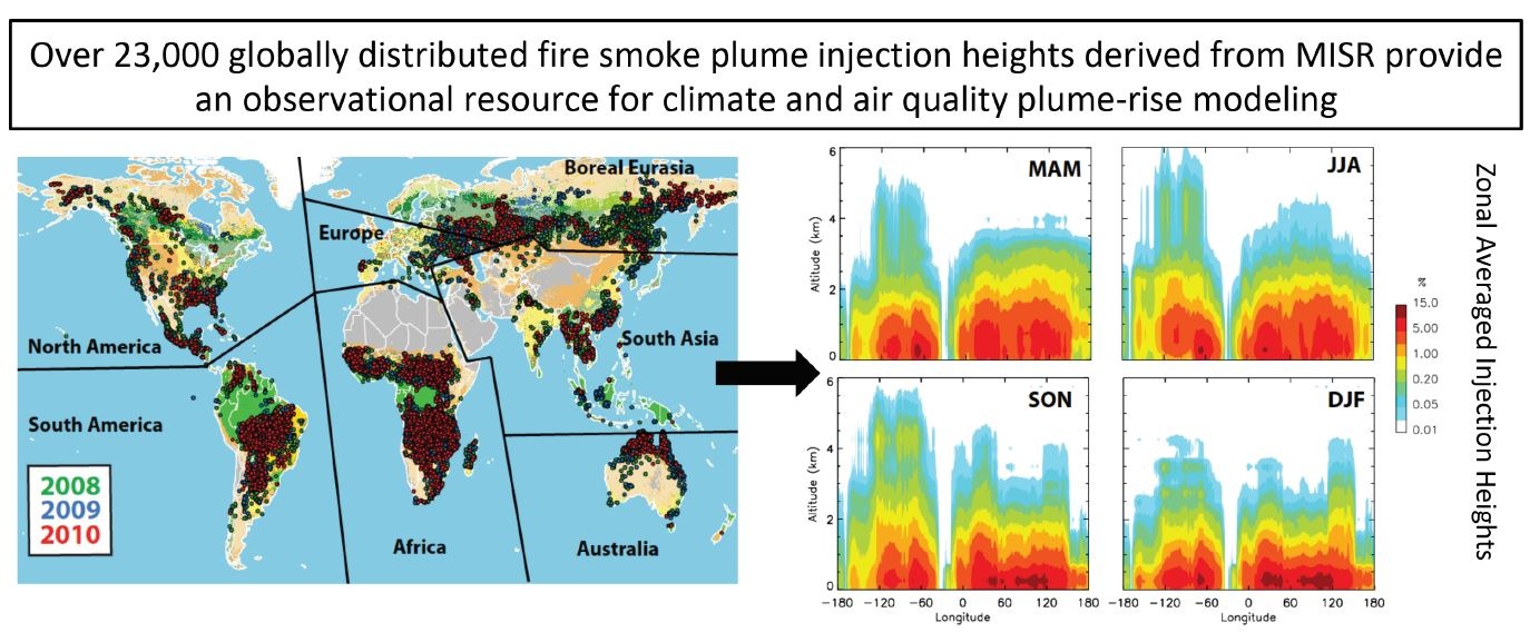
In this paper, we develop and present a 3-year record of smoke plume injection heights, stratified by region, biome, and season (Figure 1), based on over 23,000 plume heights retrieved from MISR stereo imagery. The tools used, aggregation and weighting approaches applied, and some limitations of the MISR plume-height record and our attempts at compensating for them, are discussed in Section 2. Results are given in Section 3, beginning with overall statistics on the collection of cases included in this study, then region-by-region smoke plume injection-height summaries, correlations of plume behaviour with meteorological factors, and an assessment of interannual variability. Conclusions are presented in Section 4.
2. Methodology
The primary tool used here for deriving plume heights from MISR imagery is the MISR INteractive eXplorer (MINX) software [18]. MISR flies aboard the NASA Earth Observing System’s Terra satellite, along with MODIS and three other Earth-observing instruments. MODIS 4-micron brightness temperature anomalies [19] (https://modis.gsfc.nasa.gov/data/dataprod/mod14.php) are used to help locate fires in the MISR imagery. This section summarizes the data and analysis approach used, along with the strengths and limitations of the MISR smoke plume injection-height dataset.
2.1. MISR Plume-Height Retrievals–MINX
The MISR instrument obtains imagery of each location within its 380 km-wide swath at nine view angles, ranging from 70 forward, through nadir, to 70 aft, along the orbit track, in each of four spectral bands centred at 446 (blue), 558 (green), 672 (red), and 866 nm (near infrared, NIR) wavelengths [20]. As it takes about 7 min for all nine views of a given location to be acquired, these data can be used to extract both the parallax and the proper motion of contrast features such as those in clouds and aerosol plumes [21,22]. For wildfire smoke, desert dust, and volcanic plumes in particular, more precise results can be obtained if the aerosol source, wind direction, and plume horizontal extent are specified explicitly by inspection of the imagery. The MINX tool asks an operator to provide these inputs interactively, and then calculates the wind speed and the elevation of contrast elements in the 1.1 km pixel data [18]. Both zero-wind and wind-corrected height retrievals are produced from both the red and blue-band imagery. The red-band data are acquired by MISR at 275 m horizontal resolution at all nine MISR view angles, and these provide the highest vertical resolution from the geometric retrieval approach. However, where contrast is poor within plume features and between the plume and the surface, blue-band retrievals, acquired only at 1.1 km in the MISR off-nadir cameras, usually provide better plume-element discrimination. More information about the MINX tool and digitizing examples are found in Val Martin et al. [4], Kahn et al. [10], and Nelson et al. [18].
In this work, we selected plumes digitized having “good” or “fair” MINX quality flags, with the MISR color band (i.e., blue-band or red-band retrievals) judged as superior for each digitized aerosol region given within the database. As nearly all the smoke plumes in the current study were observed over-land, blue-band retrievals yielded better quality results for 94% of the plumes in the database. In practice, vertical resolution of the MINX results is between 250 and 500 m. Heights reported by MINX are measured above mean sea level (MSL) in 250 m bins from 0 up to at least 12 km; where needed, terrain elevation must be taken into account explicitly.
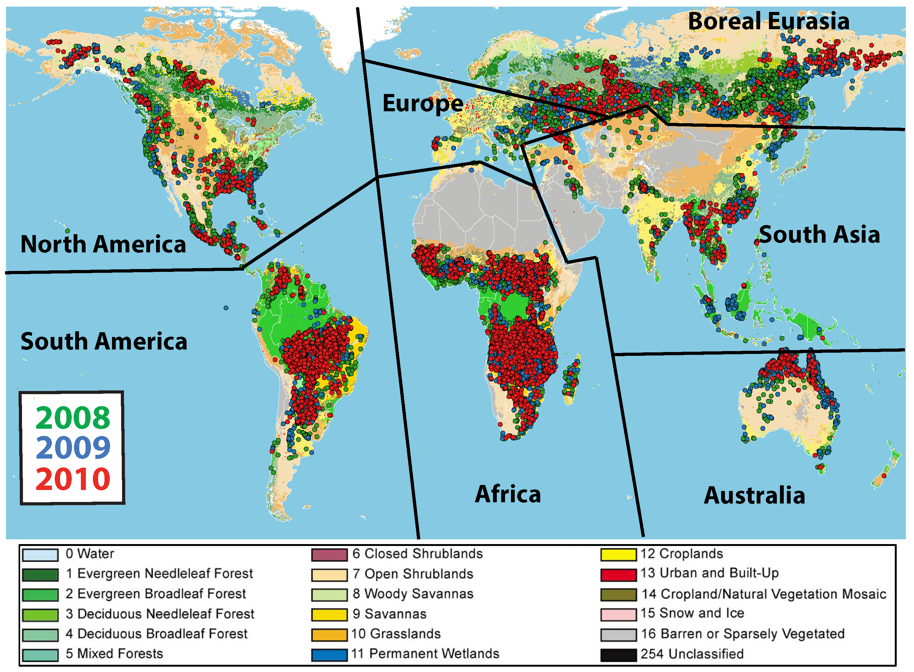
As plume digitizing with MINX is a labor-intensive process, teams of students at the Jet Propulsion Laboratory, the NASA Goddard Space Flight Center, and the University of Sheffield, UK, participated over a period of years in collecting the data used in this study (see Acknowledgments, below). Global smoke-plume data for the years 2008, 2009, and 2010 are included in the dataset. Data acquired for individual plumes were stratified by region, season, and biome, and stored by geographic region in MINX digitized aerosol region (DAR) files. Biomes are associated with geographic regions based on the Global Land-cover Types; there are 18 vegetated land-cover types from among the 22 in this database [23]. For the current study, the wildfire plumes were stratified into 12 of these biomes, covering the major vegetation types around the globe (Figure 1): Evergreen Needleleaf Forest (“EN Forest”), Evergreen Broadleaf Forest (“EB Forest”), Deciduous Needleleaf Forest (“DN Forest”), Deciduous Broadleaf Forest (“DB Forest”), “Mixed Forest”, “Closed Shrub”, “Open Shrub”, “Woody Savannah”, “Savannah”, “Grassland”, “Wetland” and “Cropland”. Plume coverage and distribution statistics for this dataset are summarized in Section 3.1 below.
2.2. Determining Stereo Height Retrieval Smoke Concentration for Individual Plumes
To develop a parameterization of fire emission injection height, we need to determine the percentage of smoke injected into different altitude bins. The distributions of AOD and smoke plume stereo-height values are both involved. For pixels within the plume having both AOD and height retrievals, we assign the AOD to the retrieved height. This assumes that the column mid-visible aerosol optical depth at 558 nm () for each pixel is concentrated in the retrieved-altitude layer of that pixel. Although this might not be true for the pixels immediately around the fire source due to the vertical extent of the smoke column, for the plume overall, smoke tends to concentrate either in the PBL or within thin (∼1 km) layers of relative atmospheric stability aloft [4,10]. With this assumption, the smoke amount at a specific elevation for the entire plume is equal to the sum of AOD values associated with all pixels in the plume region assigned to that elevation. AOD from the MISR Standard Version 22 aerosol product is reported at 17.6 km resolution and is included in the MINX output for each plume. The 1.1 km MINX pixels within the AOD retrieval region are given this value.
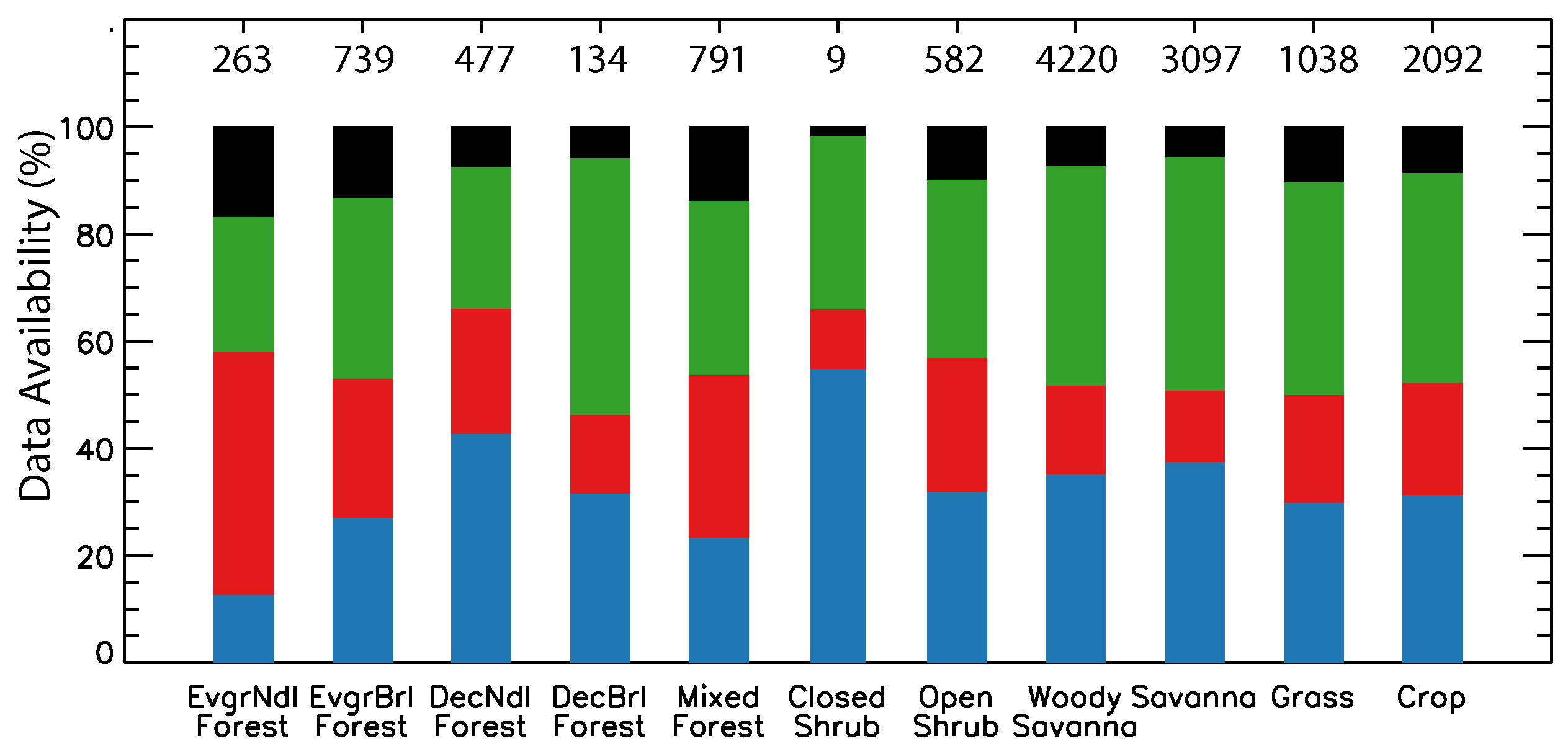
However, the distributions of smoke plume stereo-height and AOD values each can have near-source biases. The percentage of available and missing individual retrievals with AOD and stereo-height values in the dataset, stratified by biome, is shown in Figure 2. The forest biomes have fewer samples though generally bigger fires than the crop, shrub, grass, and savannah biomes. Partitioning of retrieval results also tends to vary more among the forest biomes. Overall, between about 45% and 65% of all pixels in all designated plume areas have stereo-height retrievals and between 35% and over 80% have AOD results. But only about 2–15% of all pixels are missing both AOD and height values.
This dichotomy is explained as follows: very high plume AOD favours height but not AOD retrievals, whereas low AOD favours AOD but not plume-height retrievals. Specifically, when the aerosol mid-visible optical depth exceeds a value between about 0.4 and 1, the retrieval tends to underestimate AOD [24]. Furthermore, when the AOD exceeds values around 2 or 3, the plume becomes too optically thick for the surface to be visible in the multi-angle imagery, and the AOD retrieval is altogether indeterminate. This occurs in the optically thickest parts of large plumes (see Section 2.3 below).
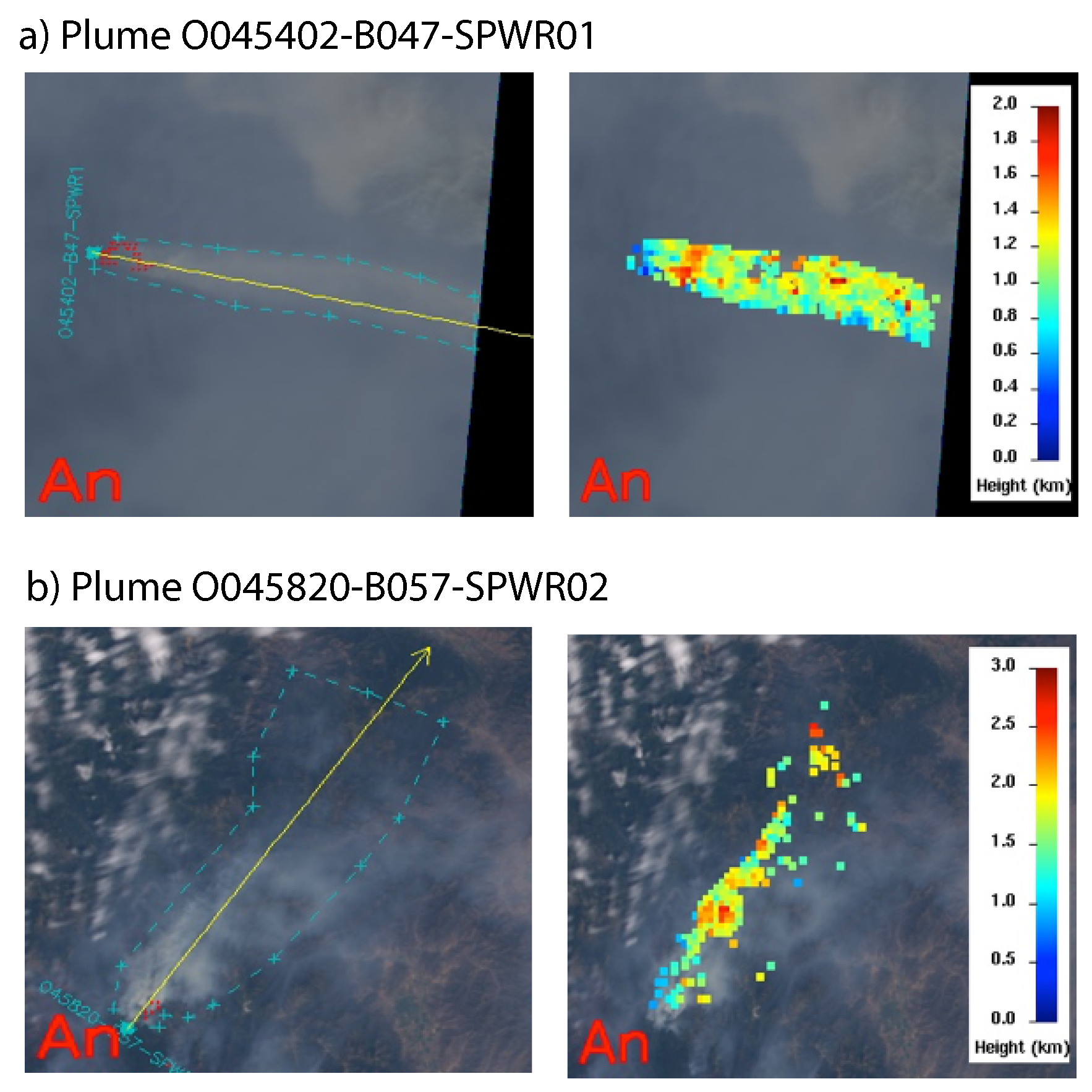
Conversely, at very low AOD, contrast features in the plume can be difficult to discern in the imagery, and stereo height retrieval becomes progressively more difficult to obtain. The specific conditions under which this occurs depend on the aerosol and the surface properties. In practice, the percent of pixels missing height retrievals depends on how much of the plume has well-defined or poorly defined features, and also on how the MINX operator defines the limits of the plume area. Picking a larger plume area, where the AOD in places might be low and the existence of the plume might be ambiguous, will yield a larger percent of pixels missing height retrievals. This is illustrated in Figure 3, which gives an example of a plume with high stereo-height retrieval density and one with low stereo-height retrieval density.
We designate the percentage of stereo heights that fills the plume area as a measure of “stereo-height retrieval density” (PcntHtsFilled in the DAR files). This density is given by the number of successful stereo-height retrievals multiplied by the area of a single retrieval pixel (1.21 km) and divided by the total area of the plume (km). We examine the relationship between mid-visible AOD and PcntHtsFilled in plumes in Figure 4, which shows the distribution of AOD relative to PcntHtsFilled for evergreen needle-leaf forest. As expected, the largest average AOD values (0.5) are associated with the largest PcntHtsFilled values (75–100%). Similar relationships are found for each biome considered in the study, except for deciduous boreal forests and grasslands (see Figure S1 in Supplemental Materials).
We aim for a practical approach that makes use of the unique information these data provide, and then characterize the uncertainties to the extent possible.
2.2.1. Pixel-Weighted Method
Filling missing stereo-height values for the current application requires an involved process. The low number of stereo heights retrieved for plumes with low PcntHtsFilled is generally associated with poor plume optical quality (i.e., low AOD, situations for which we usually have measured AOD but not height values), rather than a complete lack of smoke within the DAR. To reduce the potential bias that would occur by treating all raw individual stereo-height retrievals equally, we therefore smooth out inconsistencies among plumes characterized by different stereo-height retrieval densities using the AOD-PcntHtsFilled relationship. Our approach is to fill the non-retrieved height points within the DAR using points randomly sampled from a distribution that best fits the available retrieved height points. The underlying assumption here is that smoke elevation for locations within the plume area that do not produce height retrievals follow a height distribution statistically similar to that of the locations for which retrievals were obtained. This assumption is supported by the typically thin smoke layering downwind of the immediate source, and is explained by the extent to which the main factors determining the actual smoke plume height are affected more by initial plume buoyancy and atmospheric stability structure than by smoke amount.
To identify the statistical distributions of plume height, we carried out a fitting analysis separately for each biome. This consists of a linear regression of the dataset , , where is the MISR stereo height, is the inverse of the theoretical cumulative distribution frequency (CDF, computed numerically), N is the number of successful retrievals in a plume, and f is a function that relates to N, and depends on the type of CDF under consideration [25]. The fit analysis is conducted by testing different types of CDF (e.g., uniform, log normal, etc.). The “goodness” of fit for the sampled distribution is assessed based on the accuracy with which the versus N regression line approximates the sample. This accuracy is quantified in relation to how well the coefficient of determination approaches unity. An analysis of the robustness of this filling approach is given with Figure S2 in Supplemental Materials.
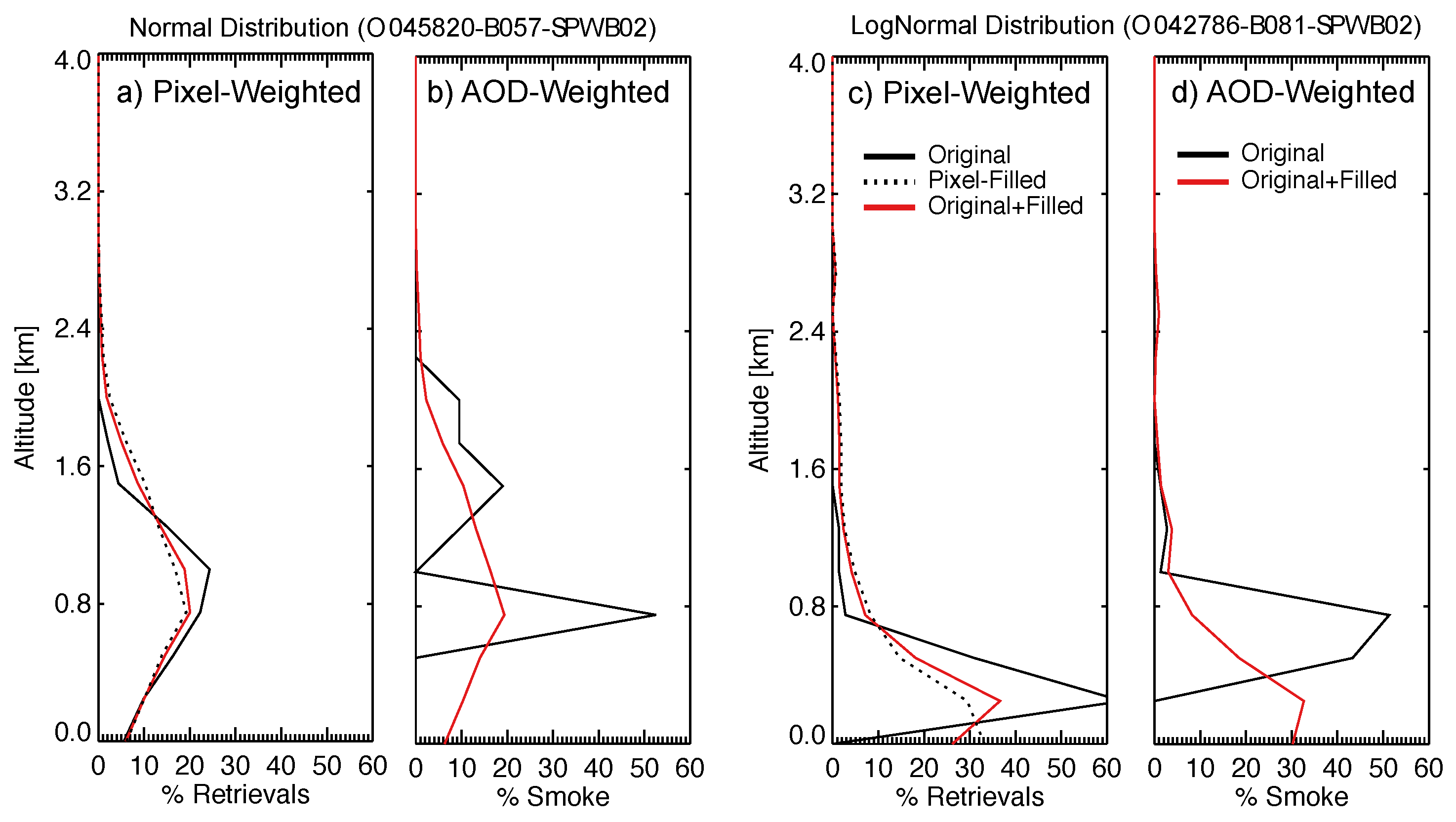
Our fitting analysis shows that for the MISR plume database, 46% of the plumes best fit a normal effective N versus height distribution, and 54% fit a lognormal distribution. The difference is probably related to differences in the vertical stability structure of the atmosphere at the altitude of the smoke layer. For example, Val Martin et al. [14] (Figures 1 and 6) show cases where normal vertical distributions are associated with weak atmospheric stability, and lognormal distributions correspond with strong stability. The values exceed 0.85, 0.90 and 0.95 for about 94%, 86%, and 58% of the plumes, respectively. For each plume, the new points are sampled from a distribution, either normal or lognormal, having the same average as the points successfully retrieved and a standard deviation calculated from that of the successful retrievals appropriately increased to account for the ±500 m measurement uncertainty associated with MISR plume heights. In addition, to avoid including points very near to or on the ground, we limit the minimum height to 250 m. Table S1 summarizes the equations used in this fitting approach. Figure 5a,c shows examples of the pixel-count-weighted vertical distribution of the stereo-height retrievals for two plumes that fit normal and lognormal distributions, respectively, with and without the smoothing approach.
2.2.2. AOD-Weighted Method
The missing AODs are most likely very high AODs, for which the retrieval fails because the surface is not visible in the multi-angle views. This is discussed in previous papers e.g., [3,10], and is evident from the observation that the missing pixel AODs occur primarily or exclusively in the thickest parts of the plumes. As such, we filled missing AOD values with the maximum AOD recorded in that plume. Lacking additional information, this provides at least lower bound on the AOD, and in most cases, the highest AOD pixels represent a small fraction of the total plume area.
As an alternative approach to determining the vertical distribution of entire plumes by simply counting the pixels at each elevation, we present the AOD-weighted vertical distribution of smoke, by calculating the percentage of smoke in each 250 m MINX vertical bin using the derived AOD values. For that, we first calculate the total AOD in each 250-m bin for the entire plume, and then determine the corresponding percentage with respect to the total column. As with the stereo-height retrievals, and to avoid including a potential bias due to missing stereo-height retrievals without AOD values, we first filled the missing AOD data with the maximum AOD recorded in each plume, as discussed above. Figure 5b,d shows examples of AOD-weighted vertical profiles with the original and original + filled AOD values.
2.3. Aggregation by Region and Biome
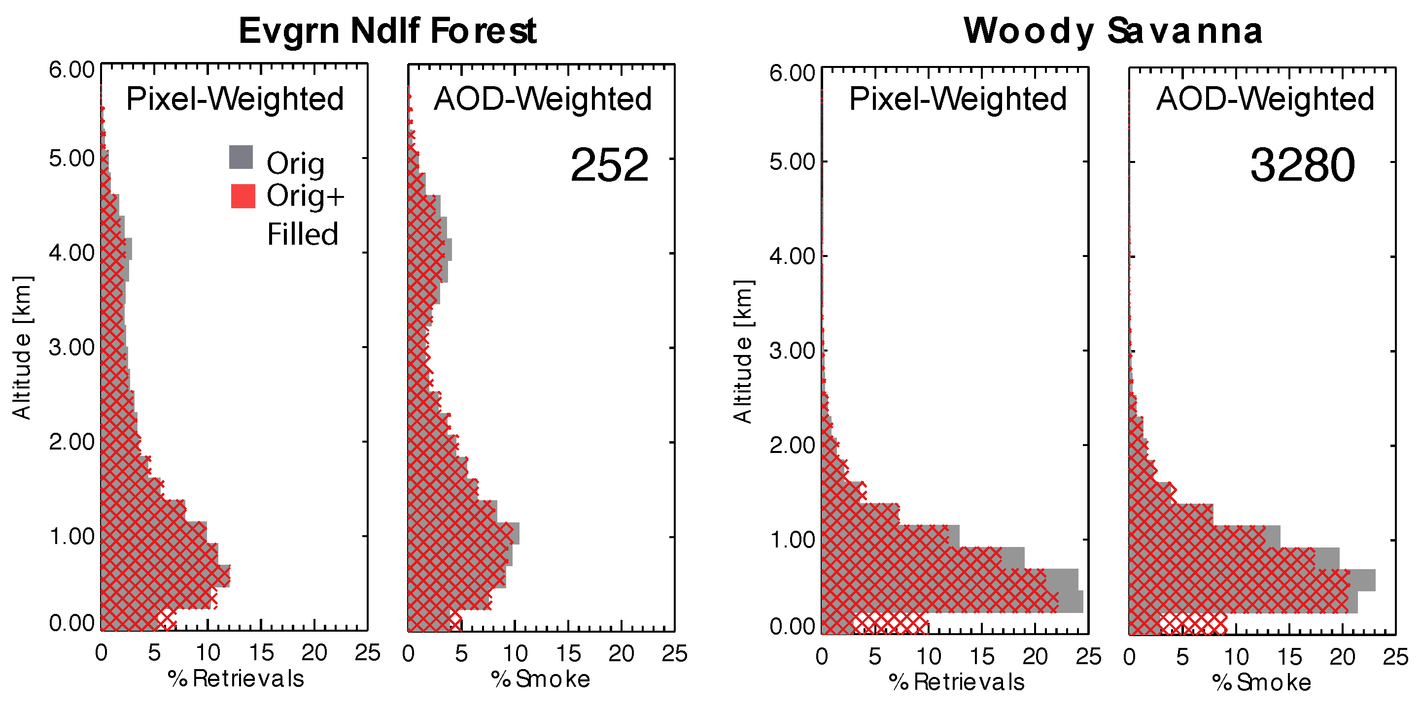
Individual cases, as treated in Section 2.2 above, are then aggregated by region and biome, giving percent injection heights at the MISR 250 m levels. Figure 6 shows examples of the normalized, pixel and AOD-weighted heights as retrieved by MISR for each 250 m altitude bin, including all the plumes over the North American mixed forest fires and African woody savannah. These are clear examples in which the filling technique yields vertical distributions of stereo-height retrievals slightly spread out towards the tails of the original distribution. This effect is important for plumes characterized by low numbers of successful retrievals. Additional vertical distributions for other biomes are given in Figures S3 and S4 in Supplemental Materials for the pixel-weighted and AOD-weighted distributions, respectively.
2.4. Limitations of the MISR Plume-Height Record Sampling
Some limitations of the MISR plume-height record sampling include: (1) the 380 km-wide MISR swath, which limits global coverage to about once per week, varying with latitude from 8 days at the equator to 2 days near the poles, (2) the day-side equator crossing time for the Terra satellite carrying the MISR instrument is 10:30 a.m., well before the afternoon peak in fire activity at most locations and during typically more stable conditions in the lower troposphere, (3) the inability to observe smoke plumes in the presence of overlying cloud cover, and (4) the lower bounds on fire and plume size that are detectable from remote sensing. There are also sampling issues that affect MODIS observation of fire pixels e.g., [3]. In addition, it is difficult to estimate the number of plumes that were missed, in part because there is no “truth” dataset with which to compare. Yet, satellites offer the best global inventory of smoke plumes currently available. A brief assessment of the biases associated with these issues, and attempts at compensating for them, are covered here.
As digitizing plumes is a labor-intensive process, some plumes may have been overlooked by the digitizers, particularly small plumes and diffuse smoke clouds. Sensitivity to the distribution of plumes varies immensely with location due to the diversity of fire types, and the numbers alone might not be a good indication of smoke abundance, for example, in areas where small-scale agricultural burning is common. As such, care has been taken to minimize missing fire events. We developed a user guide for MINX to make the digitizing process as complete and homogenous as possible [26]. Also, all the digitized plumes and most of the MISR images have passed a quality control process independent of the original digitizers. For the analysis, we only considered plumes digitized with good and fair quality so we removed from the original dataset about 15% of the digitized plumes, many of which contained only a few 1.1 km pixel retrievals, and were rendered insufficient for inclusion in the analysis.
Perhaps the best indication of missing fires is the region-specific frequency of small fires, assessed from MODIS 4-micron hot spots and suborbital data by Randerson et al. [27]. The vast majority of small fires inject smoke only into the PBL. To account for small fires that are typically under-detected by MISR, we apply a correction to the lowest level of our vertical profiles (0–250 m). Based on Randerson et al. [27], we calculate the fraction of small fires that were potentially missed by MISR, using the area burned estimated by the GFED4s inventory from large and small fires in each of our regions, biomes and burning seasons. We classify seasons as northern hemisphere spring (MAM), summer (JJA), fall (SON) and winter (DJF). Table S2 in Supplemental Materials summarizes the minimum and maximum correction fractions applied to the lowest level of our distributions to account for small fires. To normalize the distribution throughout the column, we adjust the remaining fractions evenly to sum to unity. Figure S5 shows two examples of this correction. For cropland fires over Europe during the summertime, we apply a correction of 30%, and the percentage of smoke injected in the lowest level is increased from 11.6 to 15.2%. The fraction of small fires over forests in North America is smaller (13%) and a lower increase from 5.1 to 5.7% is applied.
Validation of the multi-angle stereo-height technique is described in Nelson et al. ([18] and references therein). Further comparisons between MISR-retrieved plume heights and the vertical distribution of spatially and temporally matching smoke aerosols identified by the Cloud-Aerosol Lidar with Orthogonal Polarization (CALIOP) instrument have been done over the Amazon [28] and more are in progress [M. Tosca, personal communication]. Note that the CALIOP instrument is more sensitive to very low aerosol extinction than the MISR contrast-element technique MINX uses to derive plume heights; as such, CALIOP tends to obtain higher maximum plume heights where very thin aerosol resides above a denser aerosol layer e.g., [29].
Accounting for other MISR sampling limitations is more difficult. For example, at least a qualitative assessment of the diurnal representativeness of the MISR plume-height record might be made by comparing the FRP from Terra MODIS with corresponding values from satellites in other polar orbits, such as the MODIS instrument on NASA’s Aqua satellite that crosses the equator at 1:30 p.m. local time, and possibly geostationary FRP detectors. Such extensions would be worth exploring, but are beyond the scope of the current study.
3. Results and Discussion
We begin this section with summary statistics characterizing the plume-height dataset overall, followed by the analysis of more detailed, region-specific behaviour. The section concludes with a brief consideration of possible relationships between the observed plume injection and boundary layer height.
3.1. Smoke Plume Coverage and Distribution Statistics
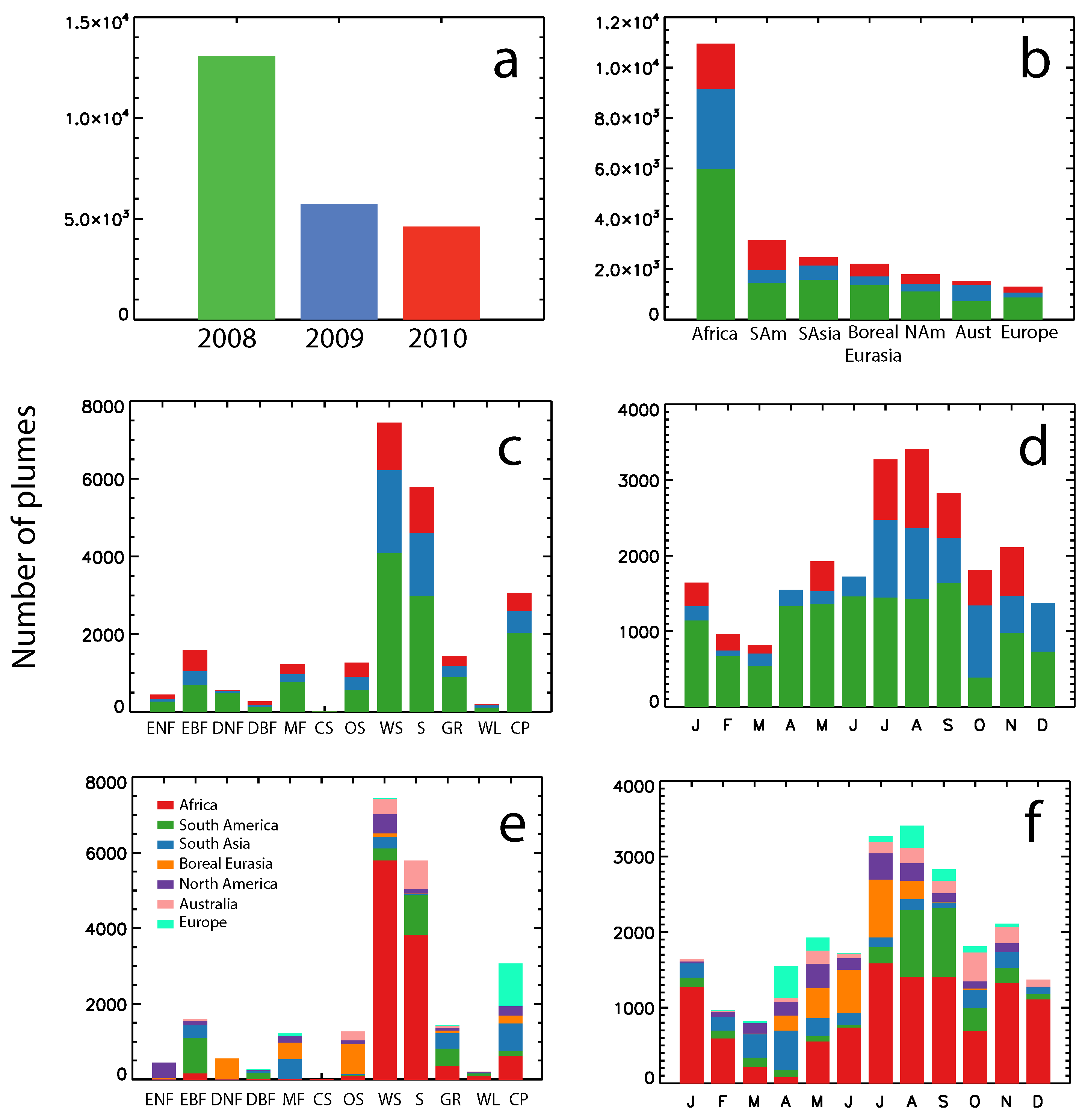
Figure 7 presents a statistical summary of the number of plumes stratified by year, month, geographic region and biome. The largest number of plumes were digitized for the year 2008, with about 13,000 plumes (56% of the total database), versus about 5700 and 4600 plumes in 2009 and 2010, respectively. We note that the 2008 plume record is missing two weeks in October (1st–16th) due to a MISR instrument technical problem and that the 2010 record includes plumes for all but three months: April, June, and December.
Most of the plumes in this database (40%) occurred between July and September (Figure 7d), which is typically the peak of the burning season in mid-latitude vegetated regions. Boreal fire counts peak in northern spring and early summer (May–July; Figure 7f). The fire season in Africa has two peaks, in northern mid-late summer (JAS) and in southern early mid-winter (NDJ). Africa is also the fire region with the largest number of plumes (47%; Figure 7b), though they are generally smaller than boreal forest fires, and tend to produce less smoke per fire. The dominant biomes in terms of fire counts are woody savannah (32%) and savannah (25%), follow by croplands (13%).
Some additional characteristics of the overall dataset are included in Supplemental Materials. In particular, Figures S6 and S7 summarize the maximum plume heights and mean AOD, respectively, stratified by region and biome, and Table S3 provides maximum height and AOD data, stratified by biome and year. Sampling varies considerably by biome and region, in part because some biomes dominate in certain regions. Furthermore, individual fires occur much more frequently in some biome types, such as savannah and cropland, than in forests. As anticipated from Figure 2, in Africa, South America, and Boreal Eurasia, the savannah, grass, and crop maximum plume-height distributions tend to be similar (Figure S6). The mean AOD, shown in Figure S7, depends in part on how the plume area is defined (e.g., Figure 3), and is much more variable than maximum height for most regions. In regions containing substantial areas of thick forest, such as North and South America and Africa, the forest biomes tend to produce the highest mean and most extreme AOD plumes, as might be expected. For Boreal Eurasia, open shrubland and woody savannah tend to produce comparably elevated plumes.
Our dataset is designed primarily to assess injection height for fires in the dominant biomes of each major biomass burning region. These are statistically well-represented in our dataset. Within the sampling limitations discussed in Section 2.4 above, the patterns suggest that we have sufficient statistics for this purpose, at least for early to mid-day local time, which is when MISR acquires data.
3.2. Global and Region-Specific Plume Injection Height Statistics
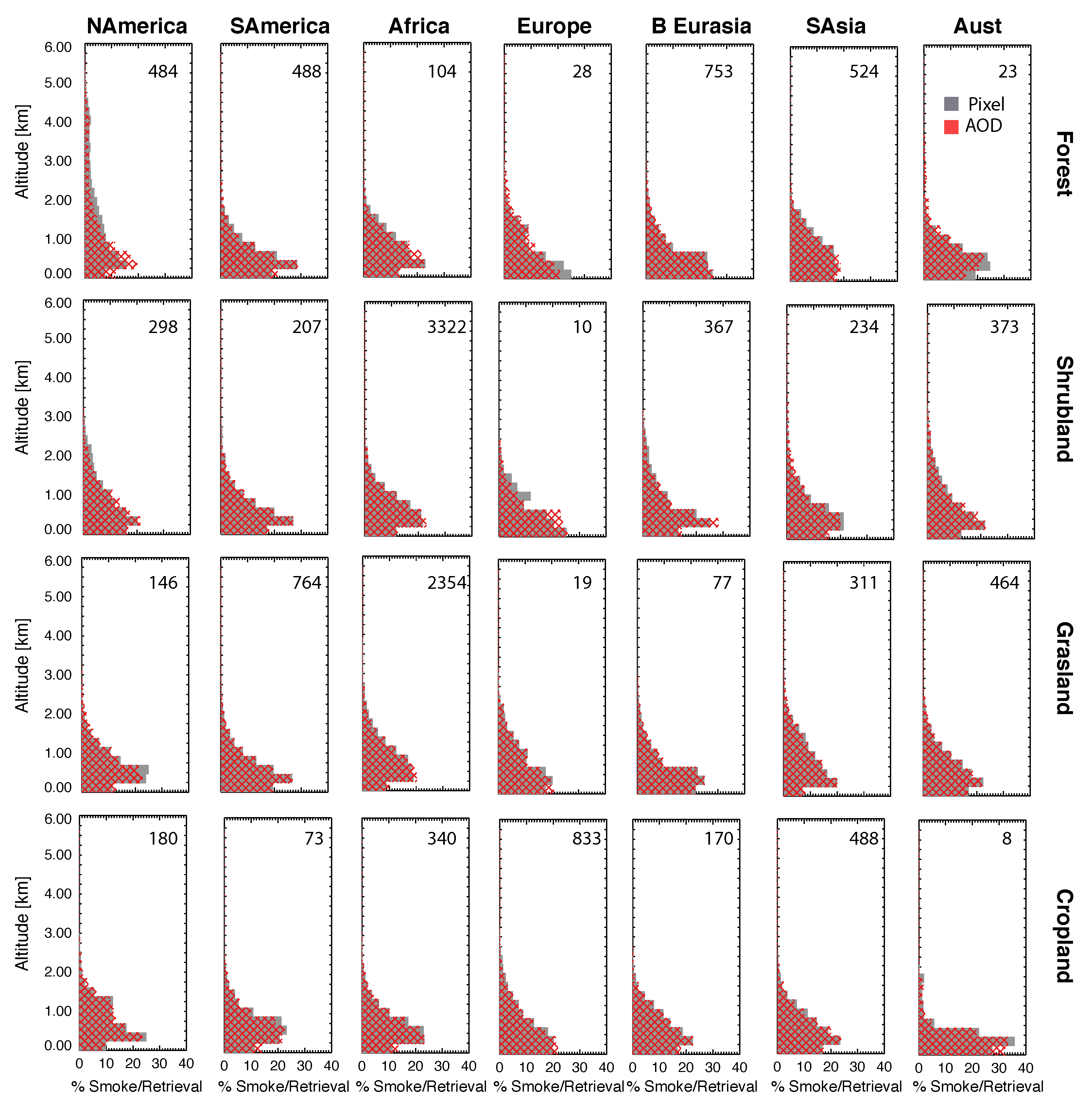
The main result of this paper is illustrated in Figure 8, which shows the AOD-weighted and pixel-weighted plume-height distributions for the entire dataset, aggregated over each of the seven primary biomass burning regions and four most widely distributed biomes in our dataset. The full AOD-weighted and pixel-weighted digital data are presented in Tables S4 and S5, respectively. Similar plots, for all 12 biomes, are given in Figures S3 and S4 in Supplemental Materials for pixel-weighted and AOD-weighted vertical distributions, respectively, with the full digital data in Table S6.
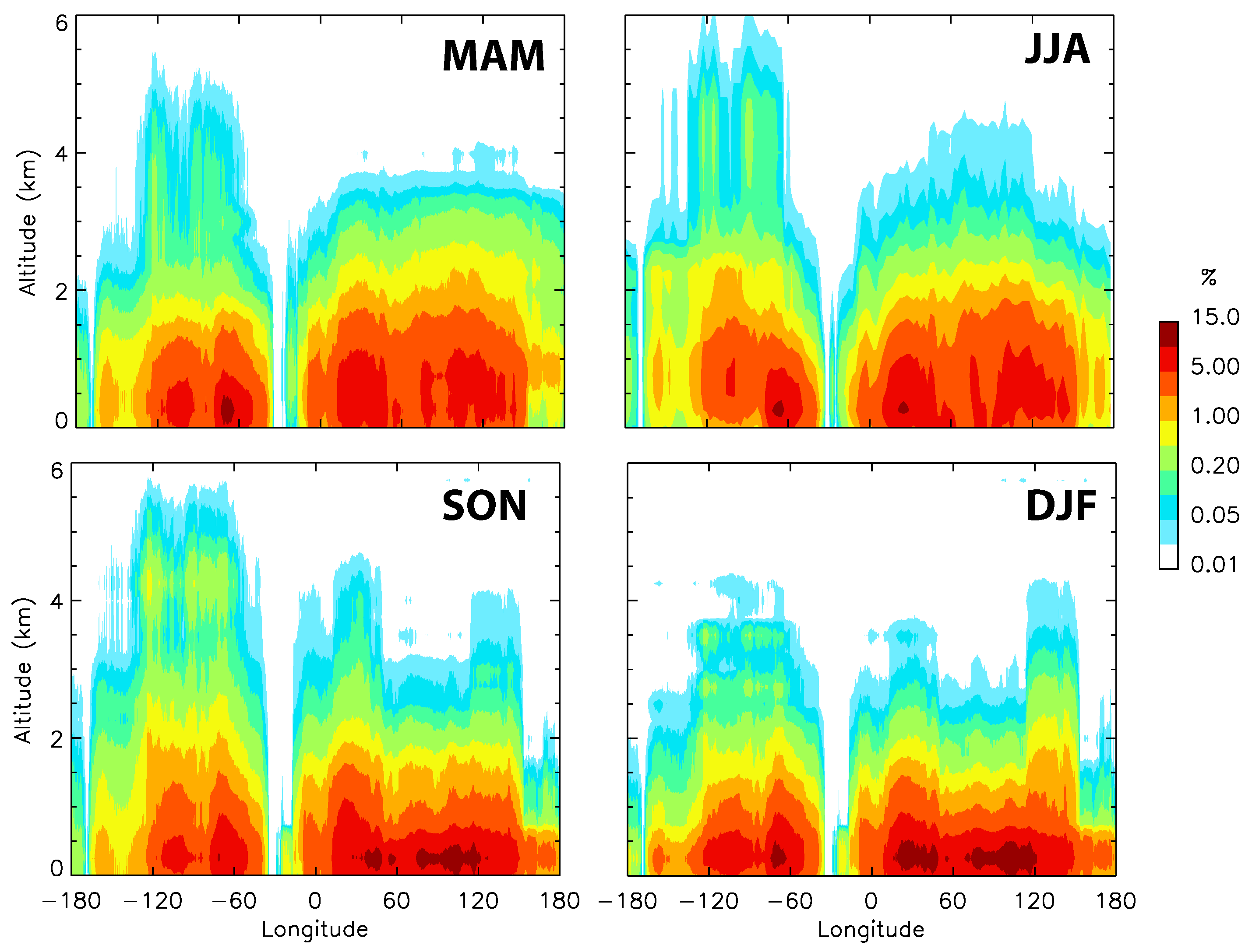
The dominance of near-surface injection is evident in Figure 8. However, smoke is injected to altitudes well above 2 km at times in nearly all the regions and biomes shown. This is easier to discern in Figure 9, which provides zonally averaged, seasonally stratified, AOD-weighted percent injection as a function of longitude and altitude. (The corresponding pixel-weighted values, and plots of the difference between AOD-weighted and pixel-weighted values, are given in Figure S8 in Supplemental Materials. There is very little difference between the AOD and pixel-weighted plots with this broad aggregation.) Averaged over the western hemisphere, smoke is injected into the mid-troposphere in northern spring, summer, and autumn, with peak heights occurring in summer, as might be expected. The eastern hemisphere produces a secondary peak in the global distribution that actually spans the entire year, and includes most of the region during northern spring and summer, but tends to be concentrated in the western and eastern extremes in autumn and winter. Injection-height seasonal variations show considerable regional dependence, and they tend to be greater in the boreal regions than in the tropics, also as expected. This appears in Figure S9 in Supplemental Materials, which presents injection heights stratified regionally for boreal North America, western US, Amazon, Sahel, Australia and Siberia. Seasonal differences are greatest over North America (where summertime boreal fires tend to be most severe), are also significant but more muted over the Sahel, Australia and Siberia, but are negligible over the Amazon.
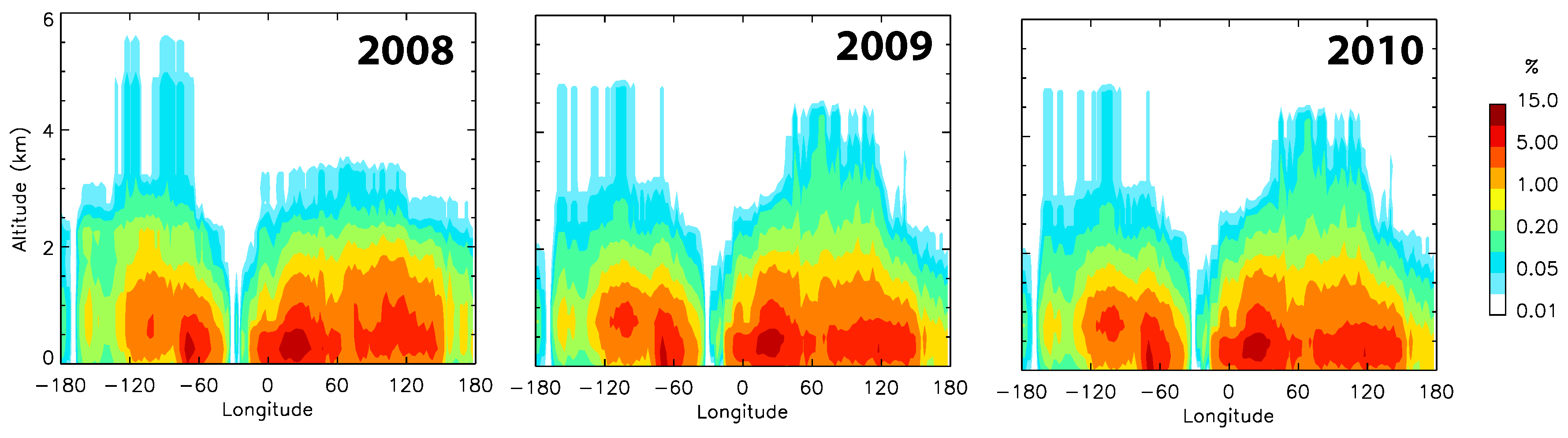
Fire severity also varies significantly from year to year, especially on a regional basis e.g., [30]. This is illustrated in Figure 10, which shows the zonally and annually averaged, AOD-weighted plume height distribution covering available data for the three years in our dataset. Interannual differences in the zonally and annually averaged plume-height distributions are given in Figure S10. Even in the averaged data, it is evident, for example, that in the western hemisphere, the peak injection heights, e.g., around longitude −120, were greater for 2008 than 2009 and 2010, corresponding to an especially severe summer fire season in California, when over 380,000 acres burned, compared to about 81,000 acres in 2009 and under 134,500 acres in 2010 [31]. In the eastern hemisphere, peak injection was less and injection was concentrated closer to the surface in 2008 than in 2009 and 2010.
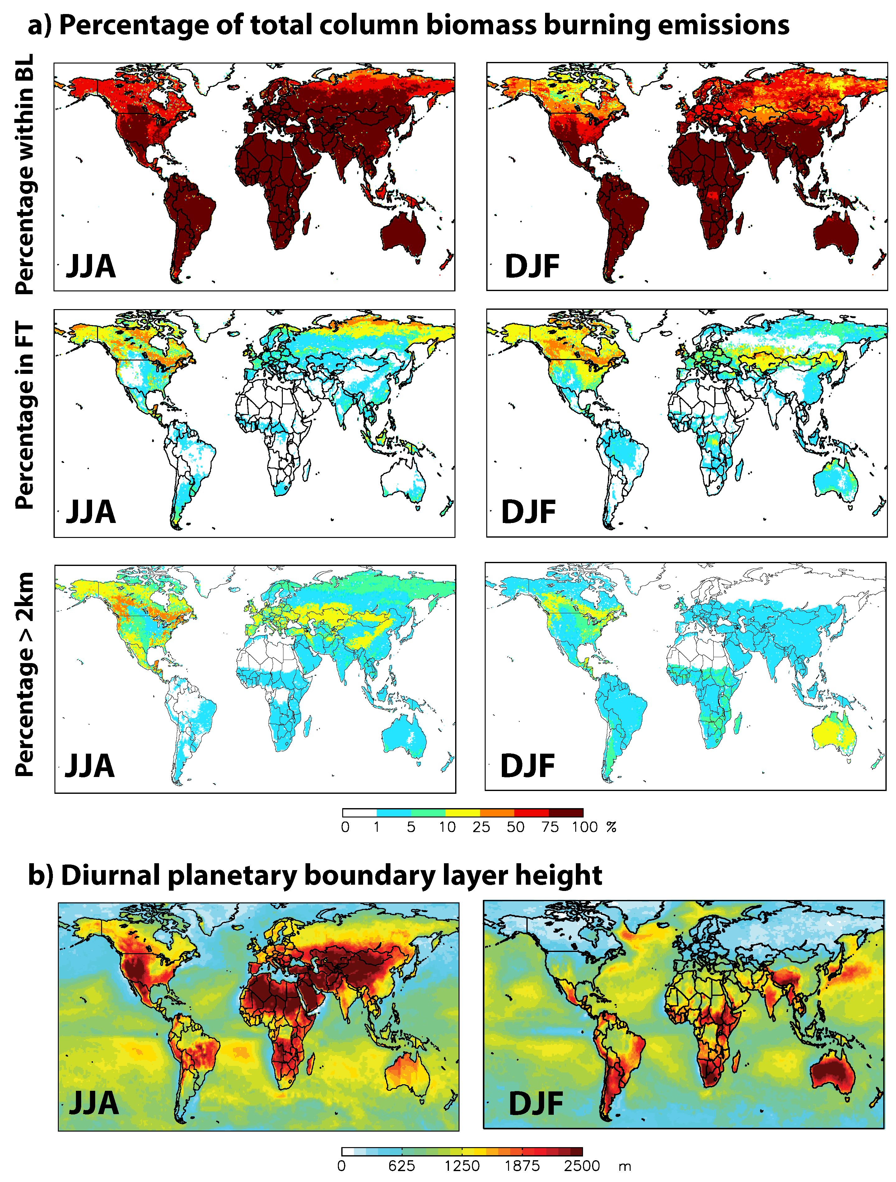
There is a deeper question that addresses when and where smoke tends to be injected above the local PBL into the free troposphere (FT). The challenge here is defining the PBL height for this application, which is not straightforward e.g., [4]. Modelling results vary, and measurements are best primarily in the few locations globally where radiosonde or LiDAR data are acquired. To make a preliminary assessment of where and when injection height above the boundary layer was more frequent, we use the PBL heights given by the second Modern Era Retrospective-analysis for Research and Applications (MERRA-2) [32], shown in Figure 11. These PBL height data are at a horizontal resolution of 0.625 longitude by 0.5 latitude and a vertical resolution of 42 levels of vertical pressure-levels between the surface and 0.01 hPa. MERRA-2 provides hourly PBL above ground level and we determine the PBL height at the time of the MISR overpass time at each MERRA grid, that is, we average the PBL heights at 10:00 a.m.–1:00 p.m. local time. Figure 11 presents one assessment of the PBL-FT injection-height dichotomy. Given the uncertainties in the plume and PBL heights, in Figure 11, we added 500 m to the nominal MERRA-2 BL height values, providing a conservative estimate of the fraction of plumes injected into the FT. We also included the percentage of smoke above 2 km altitude to provide a second metric for high-altitude smoke plume injection independent of the PBL-based definition. Globally, injection occurs most often into the PBL (and at altitudes below 2 km), and significant injection into the FT is found primarily in the boreal forests of North America and Siberia in northern summer. As the PBL itself is generally lower in the local winter season (Figure 11b), the percent injection into the FT based on the MERRA assessment expands geographically in northern winter to include parts of the eastern US and Canada, as well as parts of subtropical west Asia (Kazakhstan) and northeast China. Given the uncertainties discussed above, more detailed, regional assessments, beyond the scope of the current paper, would be needed to take advantage of the quantitative injection-height values derived from the multi-angle stereo observations e.g., [28].
4. Conclusions
We present an analysis of over 23,000 wildfire smoke plume injection heights derived from MISR space-based, multi-angle stereo imaging. The results are aimed at providing an observational resource, to complement and help improve first-principle attempts at modelling wildfire plume rise, and as a constraint on modelling smoke dispersion for climate and air quality applications. Both pixel-weighted and AOD-weighted statistics are included, and the results are stratified by region, biome, and month or season. Interannual variability is assessed by comparing the full global dataset from 2008 with partial data from 2009 and 2010, which captures moderate and severe fire seasons in different regions.
The main limitation of the dataset as a constraint on general smoke-plume-injection modelling is that diurnal coverage is precluded by the sun-synchronous MISR orbit, crossing the equator at approximately 10:30 a.m. local time on the day side. There is also a lower limit to the size of wildfires that can be detected by the spacecraft instrument, though most such fires inject smoke only into the PBL, and meteorological cloud masking underlying smoke is an issue in some regions. Missing AOD values occur preferentially in the optically thick parts of plumes, whereas missing stereo-height retrievals are found most often in the thin plume periphery. We filled the missing AOD values with the maximum AOD values observed in the plume, which provides a conservative lower bound on the actual AOD for those pixels in most cases. The missing stereo heights were filled based on the statistical distribution of observed heights for the plume in question, as the missing height retrievals tend to occur in low AOD regions towards the plume edges. These filling techniques yield stereo-height vertical distributions that are slightly spread out towards the tails of the original distributions.
Within the MISR plume database, the retrieved elevations of smoke pixels for about half the plumes are best represented as a normal distribution, whereas about half are better fit with a lognormal distribution. The difference is probably related to differences in the vertical stability structure of the atmosphere at the altitude of the smoke layer. Overall, the plumes occur preferentially (about 40% of the total) during the northern mid-latitude burning season, between July and September, but with significant regional differences (Figure 7). The savannah biomes provide the highest fire counts, whereas the heavily forested regions of North and South America, and Africa produce the highest mean and most extreme AOD plumes. Open shrubland and woody savannah in Boreal Eurasia also tend to produce comparably elevated plumes.
Figure 8 and Figures S3 and S4 in Supplemental Materials summarize the features of the database, and Tables S4–S6 in Supplemental Materials present the digital data for both pixel-weighted and AOD-weighted results. The dominance of near-surface injection is evident in these data, but some smoke is injected to altitudes well above 2 km at times in nearly all regions and biomes. Injection-height seasonal variations tend to be greater in the boreal regions than in the tropics; interannual variability is also substantial, especially on a regional basis.
Determination of PBL versus FT injection requires estimates of the PBL height, which entails additional uncertainties. We present an example using PBL heights derived from the MERRA-2 reanalysis (Figure 11); the combination of more elevated plumes and lower model-based PBL height mediates the results. This important question, which affects simulations of smoke-climate impacts as well as downwind air quality predictions warrants further study with PBL heights obtained from different sources. Recent efforts at using MISR stereo-derived plume heights to initialize model plume injection, and to begin assessing the impacts on downwind smoke dispersion, include Vernon et al. [2] and Zhu et al. [33]. The information can be also used to validate 1-D plume rise models. Vernon et al. [2] show how initializing the widely used NOAA HYSPLIT model with MISR plume heights rather than the nominal model initialization provides better simulations of smoke downwind dispersion in some cases. A comprehensive example where the MISR-based injection-height scheme is implemented and evaluated within GEOS-Chem, a major global chemical transport model, is given in Zhu et al. [33]. Further work is also indicated in terms of expanding the database. Digitizing plumes is labor-intensive [18], and fully automating the process using artificial intelligence (AI) techniques has thus far proved elusive e.g., [34]. Yet, with more than 18 years of MISR global observations, the raw data exist to strengthen the statistics presented here, to better quantify interannual variability and to derive smoke-injection-height characteristics in regions where fire plumes are less abundant in the current dataset.
Supplementary Materials
The following are available online at https://www.mdpi.com/2072-4292/10/10/1609/s1, Figure S1: Distributions of mean with respect to percentage of the DAR filled with successful retrievals (PcntHtsFilled) over 12 biomes for this study, Figure S2: Histogram of originally retrieved MISR plume heights, Figure S3: Histogram of originally retrieved MISR plume heights, originally retrieved and fitted depending on distribution type with and without ±500 m factor, and originally retrieved and fitted to a normal distribution with 1xSD and 2xSD, Figure S4: Vertical distribution of number of stereo-height retrievals in 250-m bins for successful retrievals and successful+filled retrievals (Pixel-weighted results), Figure S5: Vertical distribution of percentage of smoke in 250-m bins for original AOD retrievals and final AOD retrievals (AOD-weighted results), Figure S6: Vertical distribution of percentage of smoke calculated with the original+AOD-filled retrievals and original+AOD-filled retrievals adjusted with the GFED4s fraction to account for small fires, over cropland fire in Europe and forest fires in North America, Figure S7: MISR maximum plume height summaries by region and biome, Figure S8: MISR mean AOD by region and biome, Figure S8: Zonal (80S–80N) averages of vertical distribution of biomass burning injection heights with the pixel-weighted method for northern summer and winter, and the difference between the AOD-weighted and pixel-weighted methods, Figure S9: Regional zonal averages of vertical distribution of biomass burning injection heights with the AOD-weighted method, Figure S10: Differences in the zonal (80S–80N) annual average vertical distribution of biomass burning injection heights with the AOD-weighted method for 2008–2009 and 2008–2010, Table S1: Summary of equations used to calculate the fitting technique parameters, Table S2: Percentages (minimum and maximum) applied to the vertical distribution lowest level to account for small fires under-detected by MISR, Table S3: Statistical summary of maximum plume heights and mean AOD per biome in the MISR database, Table S4: AOD-weighted percentages of fire smoke injection heights per fire region, main biomes and seasons, Tables S5: Pixel-weighted percentages of fire smoke injection heights per fire region, broad biomes and seasons.
Author Contributions
Conceptualization, M.V.M. and R.A.K.; Methodology, M.V.M. and R.A.K.; Digitizing Plumes: M.G.T. and students (see acknowledgments); Validation, M.V.M. and R.A.K.; Formal Analysis, M.V.M.; Investigation, M.V.M. and R.A.K.; Writing—Original Draft Preparation, R.A.K.; Writing—Review & Editing, R.A.K. and M.V.M.; Supervision, R.A.K.
Funding
The work of M. Val Martin is supported by the NASA Award Number NNX14AN47G and the Leverhulme Trust through a Leverhulme Research Centre Award (RC-2015-029). The work of R. Kahn is supported in part by NASA’s Climate and Radiation Research and Analysis Program under H. Maring, NASA’s Atmospheric Composition Program under R. Eckman, and the NASA Earth Observing System’s MISR project.
Acknowledgments
Many students and some colleagues participated in digitizing plumes used in this study; in particular, we thank David Nelson, Abigail Nastan, and Laura Gonzalez-Alonso. We also thank The University of Sheffield OnCampus Placement program for supporting the digitizing effort at University of Sheffield, Y. Chen (University of California, Irvine) for the GFEDv4s data, and D. Bau (University of Sheffield) for helpful discussions about the statistical best fit analysis.
Conflicts of Interest
The authors declare no conflict of interest.
References
- Turquety, S.; Logan, J.A.; Jacob, D.J.; Hudman, R.C.; Leung, F.Y.; Heald, C.L.; Yantosca, R.M.; Wu, S.; Emmons, L.K.; Edwards, D.P.; et al. Inventory of boreal fire emissions for North America in 2004: Importance of peat burning and pyroconvective injection. J. Geophys. Res. 2007, 112, 1–13. [Google Scholar] [CrossRef]
- Vernon, C.J.; Bolt, R.; Canty, T.; Kahn, R.A. The Impact of MISR-derived Injection Height Initialization on Wildfire and Volcanic Plume Dispersion in the HYSPLIT Model. Atmos. Meas. Tech. Discuss. 2018, 2018, 1–41. [Google Scholar] [CrossRef]
- Kahn, R.A.; Chen, Y.; Nelson, D.L.; Leung, F.Y.; Li, Q.; Diner, D.J.; Logan, J.A. Wildfire smoke injection heights: Two perspectives from space. Geophys. Res. Lett. 2008, 35. [Google Scholar] [CrossRef] [Green Version]
- Val Martin, M.; Logan, J.A.; Kahn, R.A.; Leung, F.Y.; Nelson, D.L.; Diner, D.J. Smoke injection heights from fires in North America: Analysis of 5 years of satellite observations. Atmos. Chem. Phys. 2010, 10, 1491–1510. [Google Scholar] [CrossRef]
- Tosca, M.; Randerson, J.; Zender, C.; Nelson, D.; Diner, D.; Logan, J. Dynamics of fire plumes and smoke clouds associated with peat and deforestation fires in Indonesia. J. Geophys. Res. Atmos. 2011, 116. [Google Scholar] [CrossRef] [Green Version]
- Mims, S.R.; Kahn, R.A.; Moroney, C.M.; Gaitley, B.J.; Nelson, D.L.; Garay, M.J. MISR stereo heights of grassland fire smoke plumes in Australia. IEEE Trans. Geosci. Remote Sens. 2010, 48, 25–35. [Google Scholar] [CrossRef]
- Trentmann, J.; Luderer, G.; Winterrath, T.; Fromm, M.; Servranckx, R.; Textor, C.; Herzog, M.; Graf, H.F.; Andreae, M. Modeling of biomass smoke injection into the lower stratosphere by a large forest fire (Part I): Reference simulation. Atmos. Chem. Phys. 2006, 6, 5247–5260. [Google Scholar] [CrossRef]
- Peterson, D.A.; Hyer, E.J.; Campbell, J.R.; Fromm, M.D.; Hair, J.W.; Butler, C.F.; Fenn, M.A. The 2013 Rim Fire: Implications for Predicting Extreme Fire Spread, Pyroconvection, and Smoke Emissions. Bull. Am. Meteorol. Soc. 2015, 96, 229–247. [Google Scholar] [CrossRef]
- Peterson, D.; Campbell, J.; Hyer, E.; Fromm, M.; Kablick, G.; Cossuth, J.; DeLand, M. Wildfire-driven thunderstorms cause a volcano-like stratospheric injection of smoke. NPJ Clim. Atmos. Sci. 2018, 1. [Google Scholar] [CrossRef]
- Kahn, R.A.; Li, W.H.; Moroney, C.; Diner, D.J.; Martonchik, J.V.; Fishbein, E. Aerosol source plume physical characteristics from space-based multiangle imaging. J. Geophys. Res. Atmos. 2007, 112. [Google Scholar] [CrossRef] [Green Version]
- Paugam, R.; Wooster, M.; Freitas, S.; Val Martin, M. A review of approaches to estimate wildfire plume injection height within large-scale atmospheric chemical transport models. Atmos. Chem. Phys. 2016, 16, 907–925. [Google Scholar] [CrossRef] [Green Version]
- Ichoku, C.; Kaufman, Y.J. A method to derive smoke emission rates from MODIS fire radiative energy measurements. IEEE Trans. Geosci. Remote Sens. 2005, 43, 2636–2649. [Google Scholar] [CrossRef]
- Ichoku, C.; Ellison, L. Global top-down smoke-aerosol emissions estimation using satellite fire radiative power measurements. Atmos. Chem. Phys. 2014, 14, 6643–6667. [Google Scholar] [CrossRef] [Green Version]
- Val Martin, M.; Kahn, R.A.; Logan, J.A.; Paugam, R.; Wooster, M.; Ichoku, C. Space-based observational constraints for 1-D fire smoke plume-rise models. J. Geophys. Res. Atmos. 2012, 117. [Google Scholar] [CrossRef] [Green Version]
- Garratt, J. Review: The atmospheric boundary layer. Earth-Sci. Rev. 1994, 37, 89–134. [Google Scholar] [CrossRef]
- Freitas, S.R.; Longo, K.M.; Chatfield, R.; Latham, D.; Silva Dias, M.; Andreae, M.; Prins, E.; Santos, J.; Gielow, R.; Carvalho, J., Jr. Including the sub-grid scale plume rise of vegetation fires in low resolution atmospheric transport models. Atmos. Chem. Phys. 2007, 7, 3385–3398. [Google Scholar] [CrossRef] [Green Version]
- Kukkonen, J.; Nikmo, J.; Sofiev, M.; Riikonen, K.; Petäjä, T.; Virkkula, A.; Levula, J.; Schobesberger, S.; Webber, D.M. Applicability of an integrated plume rise model for the dispersion from wild-land fires. Geosci. Model Dev. 2014, 7, 2663–2681. [Google Scholar] [CrossRef] [Green Version]
- Nelson, D.L.; Garay, M.J.; Kahn, R.A.; Dunst, B.A. Stereoscopic height and wind retrievals for aerosol plumes with the MISR INteractive eXplorer (MINX). Remote Sens. 2013, 5, 4593–4628. [Google Scholar] [CrossRef]
- Giglio, L.; Van der Werf, G.; Randerson, J.; Collatz, G.; Kasibhatla, P. Global estimation of burned area using MODIS active fire observations. Atmos. Chem. Phys. 2006, 6, 957–974. [Google Scholar] [CrossRef] [Green Version]
- Diner, D.J.; Beckert, J.C.; Reilly, T.H.; Bruegge, C.J.; Conel, J.E.; Kahn, R.A.; Martonchik, J.V.; Ackerman, T.P.; Davies, R.; Gerstl, S.A.; et al. Multi-angle Imaging SpectroRadiometer (MISR) instrument description and experiment overview. IEEE Trans. Geosci. Remote Sens. 1998, 36, 1072–1087. [Google Scholar] [CrossRef]
- Moroney, C.; Davies, R.; Muller, J.P. Operational retrieval of cloud-top heights using MISR data. IEEE Trans. Geosci. Remote Sens. 2002, 40, 1532–1540. [Google Scholar] [CrossRef]
- Muller, J.P.; Mandanayake, A.; Moroney, C.; Davies, R.; Diner, D.J.; Paradise, S. MISR stereoscopic image matchers: Techniques and results. IEEE Trans. Geosci. Remote Sens. 2002, 40, 1547–1559. [Google Scholar] [CrossRef]
- Bartholomé, E.; Belward, A.S. GLC2000: A new approach to global land cover mapping from Earth observation data. Int. J. Remote Sens. 2005, 26, 1959–1977. [Google Scholar] [CrossRef]
- Kahn, R.A.; Gaitley, B.J.; Garay, M.J.; Diner, D.J.; Eck, T.F.; Smirnov, A.; Holben, B.N. Multiangle Imaging SpectroRadiometer global aerosol product assessment by comparison with the Aerosol Robotic Network. J. Geophys. Res. Atmos. 2010, 115. [Google Scholar] [CrossRef] [Green Version]
- Hahn, G.J.; Shapiro, S.S. Statistical Models in Engineering; John Wiley & Sons, Inc.: New York, NY, USA, 1994. [Google Scholar]
- Nelson, D.L.; Chen, Y.; Kahn, R.A.; Diner, D.J.; Mazzoni, D. Example applications of the MISR INteractive eXplorer (MINX) software tool to wildfire smoke plume analyses. In Proceedings of the SPIE Remote Sensing of Fire: Science and Application, San Diego, CA, USA, 10–14 August 2008; Volume 7089, pp. 708909.1–708909.11. [Google Scholar] [CrossRef]
- Randerson, J.T.; Chen, Y.; Werf, G.R.; Rogers, B.M.; Morton, D.C. Global burned area and biomass burning emissions from small fires. J. Geophys. Res. Biogeosci. 2012, 117. [Google Scholar] [CrossRef] [Green Version]
- Gonzalez-Alonso, L.; Val Martin, M.; Kahn, R.A. Biomass burning smoke heights over the Amazon observed from space. Atmos. Chem. Phys. Discuss. 2018. [Google Scholar] [CrossRef]
- Flower, V.J.; Kahn, R.A. Assessing the altitude and dispersion of volcanic plumes using MISR multi-angle imaging from space: Sixteen years of volcanic activity in the Kamchatka Peninsula, Russia. J. Volcanol. Geotherm. Res. 2017, 337, 1–15. [Google Scholar] [CrossRef]
- Williamson, G.J.; Prior, L.D.; Jolly, W.M.; Cochrane, M.A.; Murphy, B.P.; Bowman, D.M.J.S. Measurement of inter- and intra-annual variability of landscape fire activity at a continental scale: The Australian case. Environ. Res. Lett. 2016, 11, 035003. [Google Scholar] [CrossRef]
- CalFire. Cal Fire Web Site. 2018. Available online: http://www.fire.ca.gov/fire_protection/fire_protection_fire_info_redbooks (accessed on 24 August 2018).
- Bosilovich, M.G.; Lucchesi, R.; Suarez, M. MERRA-2: File Specification. GMAO Office Note No. 9 (Version 1.1); 2016. Available online: http://gmao.gsfc.nasa.gov/pubs/office_notes (accessed on 24 August 2018).
- Zhu, L.; Val Martin, M.; Hecobian, A.; Gatti, L.V.; Kahn, R.; Fischer, E.V. Development and implementation of a new biomass burning emissions injection height scheme for the GEOS-Chem model. Geosci. Model Dev. Discuss. 2018, 2018, 1–30. [Google Scholar] [CrossRef]
- Mazzoni, D.; Logan, J.A.; Diner, D.; Kahn, R.; Tong, L.; Li, Q. A data-mining approach to associating MISR smoke plume heights with MODIS fire measurements. Remote Sens. Environ. 2007, 107, 138–148. [Google Scholar] [CrossRef] [Green Version]
Figure 1.
Geographic regions used in this study, and associated land-cover types, with dots indicating individual cases included in the dataset.
Figure 1.
Geographic regions used in this study, and associated land-cover types, with dots indicating individual cases included in the dataset.

Figure 2.
Data availability in the 2008 plume dataset determined per biome. Bars represent percentage of individual pixels with both stereo-height and AOD retrievals (blue), percentage with height but missing AOD retrievals (red), percentage with AOD but missingstereo-height retrievals (green) and percentage with missing both stereo-height and AOD retrievals (black). The number of plumes included in each distribution is given above the bar plots.

Figure 3.
Examples of Plume Stereo-height Retrieval Density. (a) Plume O045402-B047-SPWR01 with high retrieval density (PtctHtsFilled = 84%) and high AOD (mean AOD558 = 1.05); (b) Plume O045820-B057-SPWR02 with low retrieval density (PtctHtsFilled = 40%) and lower AOD (mean AOD558 = 0.2).
Figure 3.
Examples of Plume Stereo-height Retrieval Density. (a) Plume O045402-B047-SPWR01 with high retrieval density (PtctHtsFilled = 84%) and high AOD (mean AOD558 = 1.05); (b) Plume O045820-B057-SPWR02 with low retrieval density (PtctHtsFilled = 40%) and lower AOD (mean AOD558 = 0.2).

Figure 4.
Distribution of mean AOD with respect to percentage of the DAR filled with successful retrievals (PcntHtsFilled) over evergreen needle-leaf forest. The medians (red circles) and the means (black squares) are shown along with the central 67% (light blue box) and the central 90% (black whiskers). Similar plots for other biomes are given in Figure S1 in Supplemental Materials. The number of cases is indicated at the top of each boxplot.

Figure 5.
Examples of stereo-height retrieval vertical distributions for smoke plumes with normal (O045820-B057-SPWB02, shown in Figure 3 bottom row; panels (a,b) here) and lognormal (O042786-B081-SPWB02; panels (c,d) here) distribution fits. (a,c) Distributions weighted by pixel counts. Solid black lines indicate original successful retrievals, dashed black lines represent missing retrievals that were filled as described in Section 2.2, and red lines are the sum of original and filled retrievals. (b,d) Distributions weighted by AOD. Solid black lines indicate original retrievals with AOD values, and red lines are the sum of original AOD and filled retrievals, in which missing AOD values were filled by the maximum AOD in each plume.

Figure 6.
Vertical distribution of percentage of pixel-weighted and AOD-weighted stereo-height retrievals in 250-m bins for original retrievals (grey) and the missing height and AOD-filled retrievals (hatched red), over North American evergreen needle-leaf forest and African woody savannah. Numeric annotations indicate the number of plumes in each classification.

Figure 7.
Summary of the MISR plume-height database stratified by (a) year, (b) region and year, (c) biome and year, (d) month and year, (e) biome and region, and (f) month and region. The 12 biomes included in this dataset are listed at the end of Section 2.1, and illustrated in Figure 1.
Figure 7.
Summary of the MISR plume-height database stratified by (a) year, (b) region and year, (c) biome and year, (d) month and year, (e) biome and region, and (f) month and region. The 12 biomes included in this dataset are listed at the end of Section 2.1, and illustrated in Figure 1.

Figure 8.
Vertical distribution of percentage of pixel-weighted (grey) and AOD-weighted (hatched red) stereo-height retrievals in 250-m bins. Profiles show the stereo-height retrievals pixel-filled and AOD-filled and adjusted by the GFED4s to account small fires. Numeric annotations indicate the number of plumes in each classification.

Figure 9.
Zonal (80S–80N) averages of vertical distribution of biomass burning injection heights with the AOD-weighted method (%) for northern spring (MAM), summer (JJA), fall (SON) and winter (DJF). The 2008 data were used for these plots.
Figure 9.
Zonal (80S–80N) averages of vertical distribution of biomass burning injection heights with the AOD-weighted method (%) for northern spring (MAM), summer (JJA), fall (SON) and winter (DJF). The 2008 data were used for these plots.

Figure 10.
Zonal (80S–80N) annual averages of vertical distribution of biomass burning injection heights with the AOD-weighted method (%) for 2008, 2009 and 2010.
Figure 10.
Zonal (80S–80N) annual averages of vertical distribution of biomass burning injection heights with the AOD-weighted method (%) for 2008, 2009 and 2010.

Figure 11.
Percentage of total column biomass burning emissions injected into the PBL and into the FT (above PBL + 500 m to 6 km and above 2 km to 6 km) in each grid cell based on the estimated AOD-weighted injection heights (a) and global diurnal planetary boundary layer height from MERRA-2 (b). Hourly PBL heights were average from 10:00 a.m. to 1:00 p.m. (LT) to represent the MISR overpass time over the regions. Results are shown for northern summer (JJA) and winter (DJF).

© 2018 by the authors. Licensee MDPI, Basel, Switzerland. This article is an open access article distributed under the terms and conditions of the Creative Commons Attribution (CC BY) license (http://creativecommons.org/licenses/by/4.0/).
Share and Cite
MDPI and ACS Style
Val Martin, M.; Kahn, R.A.; Tosca, M.G. A Global Analysis of Wildfire Smoke Injection Heights Derived from Space-Based Multi-Angle Imaging. Remote Sens. 2018, 10, 1609. https://doi.org/10.3390/rs10101609
AMA Style
Val Martin M, Kahn RA, Tosca MG. A Global Analysis of Wildfire Smoke Injection Heights Derived from Space-Based Multi-Angle Imaging. Remote Sensing. 2018; 10(10):1609. https://doi.org/10.3390/rs10101609
Chicago/Turabian StyleVal Martin, Maria, Ralph A. Kahn, and Mika G. Tosca. 2018. "A Global Analysis of Wildfire Smoke Injection Heights Derived from Space-Based Multi-Angle Imaging" Remote Sensing 10, no. 10: 1609. https://doi.org/10.3390/rs10101609
Note that from the first issue of 2016, this journal uses article numbers instead of page numbers. See further details here.