Quantitative Identification of Maize Lodging-Causing Feature Factors Using Unmanned Aerial Vehicle Images and a Nomogram Computation

Abstract

Maize (zee mays L.) is one of the most important grain crops in China. Lodging is a natural disaster that can cause significant yield losses and threaten food security. Lodging identification and analysis contributes to evaluate disaster losses and cultivates lodging-resistant maize varieties. In this study, we collected visible and multispectral images with an unmanned aerial vehicle (UAV), and introduce a comprehensive methodology and workflow to extract lodging features from UAV imagery. We use statistical methods to screen several potential feature factors (e.g., texture, canopy structure, spectral characteristics, and terrain), and construct two nomograms (i.e., Model-1 and Model-2) with better validation performance based on selected feature factors. Model-2 was superior to Model-1 in term of its discrimination ability, but had an over-fitting phenomenon when the predicted probability of lodging went from 0.2 to 0.4. The results show that the nomogram could not only predict the occurrence probability of lodging, but also explore the underlying association between maize lodging and the selected feature factors. Compared with spectral features, terrain features, texture features, canopy cover, and genetic background, canopy structural features were more conclusive in discriminating whether maize lodging occurs at the plot scale. Using nomogram analysis, we identified protective factors (i.e., normalized difference vegetation index, NDVI and canopy elevation relief ratio, CRR) and risk factors (i.e., Hcv) related to maize lodging, and also found a problem of terrain spatial variability that is easily overlooked in lodging-resistant breeding trials.

1. Introduction

Maize (zee mays L.) is one of the most important grain crops in China, used as food, fodder, and bioenergy. The planting area and yield of maize are 35.445 million hectares and 215.891 million tons, respectively, in 2017, ranking first among staple crops, reported by the National Bureau of Statistics [1]. Lodging is one of the main reasons contributing to the yield reduction and quality deterioration of various crops [2,3]. Furthermore, lodging resistance is not only the main breeding target for crop improvement [4], but also an important phenotypic trait in field investigation. Advances in agronomic and breeding efforts to improve lodging resistance and protect the food supply security have been limited by traditional field phenotyping methods [5,6].

Traditional field phenotyping relies on ground investigation using manpower measurement, which is expensive, laborious, and inefficient, especially when thousands of plots are being evaluated in a breeding program [7,8], and it is not applicable to large scale and repeatable surveys [9]. With the richness of platforms and sensors, remote sensing technology provides a feasible, reliable, and valid approach to identify and analyze crop lodging [6,10,11]. A satellite remote sensing platform covers a large area, but it is limited in revisiting time, and there is a trade-off between spatial and spectral resolution [12]. Compared with a satellite platform, an unmanned aerial vehicle (UAV) platform with proper sensors offers a flexible, low-cost, and high-resolution solution to monitoring the lodging within a relatively small area [6]. Different types of sensors are being used to identify distinguishable features (i.e., lodging and non-lodging features) of crops lodging. Yang et al. [13] reported that polarimetric features extracted from synthetic aperture radar (SAR) imagery were used to monitor wheat lodging. Han et al. [9] reported that the ratio of the natural height to the plant height extracted from SAR imagery was used as a standard for distinguishing the degree of lodging. Liu et al. [14] and Li et al. [15] reported that spectral features were utilized to estimate the lodging grade by using multispectral sensors. Based on digital images and multispectral images, Liu et al. [16] combined spectra with texture feature to identify the area of wheat lodging. Li et al. [11] and Yang et al. [17] reported on texture features and color features extracted from UAV digital imagery that were used for lodging area assessment. By using a thermal infrared sensor, Liu et al. [6] determined that the temperature was distinct between lodging and non-lodging areas, with lodging rice having a higher canopy temperature. Navabi et al. [18] reported that lodging severity was positively correlated with plant height in a diverse wheat population. Chu et al. [10] proposed a method to assess lodging severity over an experimental maize field by using a digital camera and plant height information.

In different scenarios, it is generally impossible to determine in advance which feature can effectively distinguish between lodging and non-lodging areas, so it is necessary to screen the features. In fact, the features extracted from the imagery are all affected by interfering factors such as soil background, weather conditions, observation time, and mixed pixels. Due to the limitation of these interfering factors, using a single feature to identify and analyze lodging may not be sufficient. It is worth studying deeply to identify lodging and determine the strength of the effect that feature factors have on maize lodging based on multiple feature factors.

Logistic regression was developed by statistician David Cox [19], which was used to explain the relationship between one dependent nominal variable (i.e., outcome) and one or more continuous-level (interval or ratio scale) predictor variables [20,21]. A nomogram is a two-dimensional diagram that allows the approximate graphical representation of a logistic regression model, which has a long history in engineering and medicine [22]. In the medical diagnostic research, logistic regression and nomograms as the statistical analysis methods are widely used to analyze post-operative survival prediction and to screen for risk factors [23,24,25].

Few studies have employed multiple feature factors provided by UAV remote sensing to identify maize lodging and analyze the strength effect of feature factors in a maize breeding program. Therefore, the main objectives of this study are: (1) to introduce a comprehensive methodology and workflow to extract lodging multiple features from UAV imagery, (2) to screen the lodging features factors by using a logistic regression analysis method, (3) to construct a nomogram to predict the occurrence probability of lodging and explore the underlying association between maize lodging and the selected predictors, and (4) to explore the potential of breeding phenotypic traits using UAV remote sensing.

2. Material and Methodology

2.1. Study Area and Field Measurement

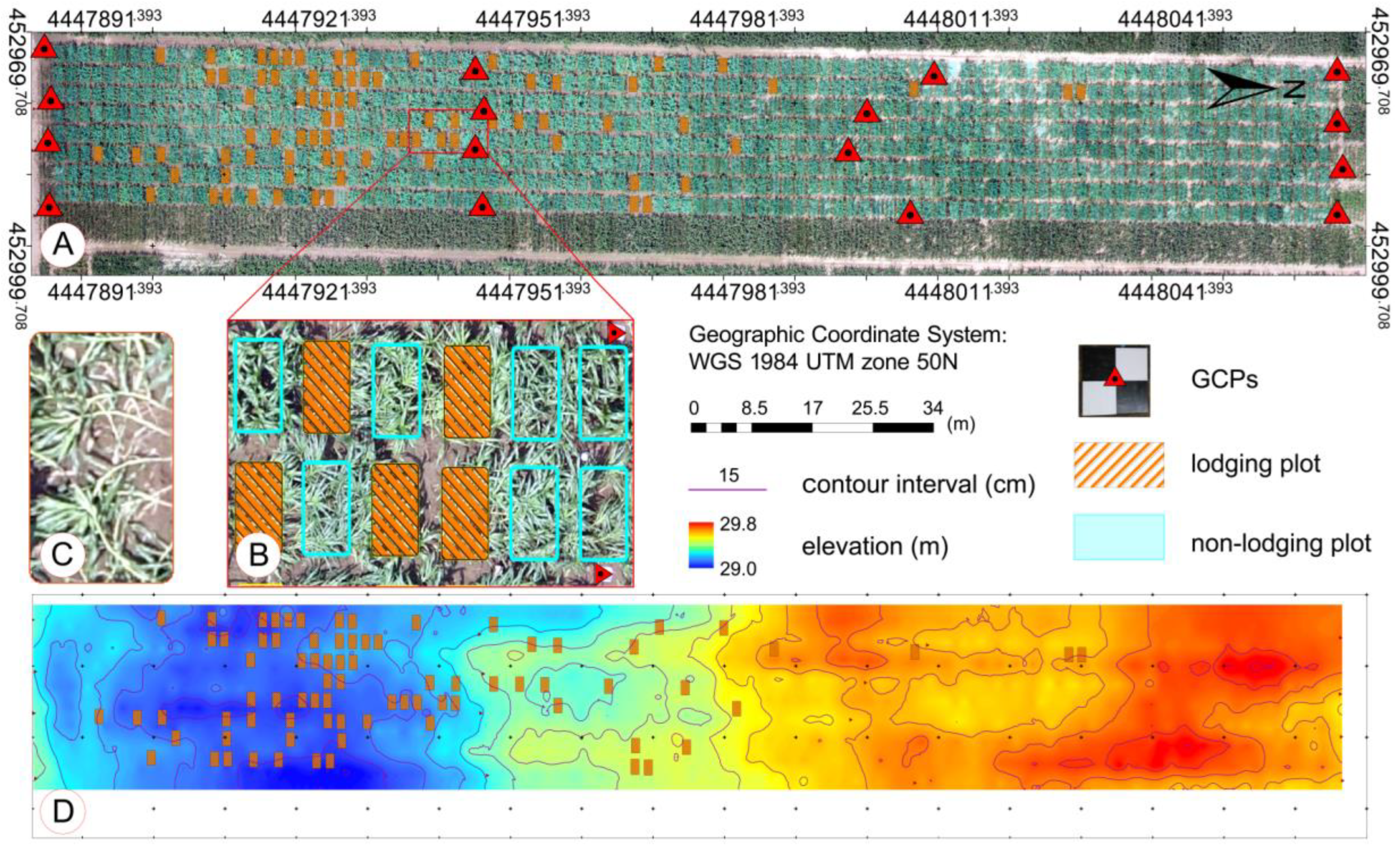
The field trial was conducted at the research station of Xiao Tangshan National Precision Agriculture Research Center of China, which covers an area of about two square kilometers and is located in the Changping District of Beijing City. The trial area was approximately 210 m from north to south and approximately 27 m from east to west. A single factor breeding trial with the randomized block design was adopted in this study. Maize seeds of different genetic backgrounds with differences in growth period and stalk stiffness were sown on 15 May 2017. Eight hundred maize breeding plots with a size of 2.4 m × 2 m were arranged in 100 rows and 8 columns and used to observe the phenotypic expression of maize. These plots were planted using a seeding density of 6 plants/m² and a row spacing of 0.6 m. To extract the plant height from UAV images accurately, 16 ground control points (GCPs) were distributed evenly within the field (Figure 1) and measured with a differential global positioning system (DGPS, South Surveying & Mapping Instrument Co., Ltd., Shenzhen, China) with millimeter accuracy. The GCPs were marked with 50 cm × 50 cm, black and white, square planks were nailed to a stake stably fixed in the ground. Meteorological data were acquired from QT-1060 open-path eddy-covariance systems (Channel Technology Group Limited, Beijing, China) in the field. From 1 to 10 July, there were several strong winds and rainfall, and the daily average precipitation reached 7.6 mm, which resulted in the lodging of maize on 11 July 2017. It was then that maize in the trial area was at the growth stage 19 (BBCH-scale) [26].

In 72 sampling plots, plant height was measured manually by a telescopic leveling rod. Avoiding the influence of marginal effects and growth competition, the average of the three plants in the center of each sampling plot was counted as the representative value for the ground truth of plant height. Removing 11 sampling plots affected by lodging from 72 sampling plots, 61 sampling plots were used to validate plant height extraction accuracy.

2.2. UAV Flight and Image Processing

A Sony Cyber-shot DSC-QX100 (Sony Electronics Inc., Tokyo, Japan) camera (resolution: 5472 × 3648 pixels) served as an optical sensor to record RGB images and a Parrot Sequoia (MicaSense Inc., Seattle, WA, USA) camera (resolution: 1280 × 960 pixels, four different spectral bands: green (wavelength 550 nm; bandwidth 40 nm), red (wavelength 660 nm; bandwidth 40 nm), red-edge (wavelength 735 nm; bandwidth 10 nm) and near infrared (wavelength 790 nm; bandwidth 40 nm)) served as a multispectral sensor to acquire spectral images, were mounted on a DJI Spreading Wings S1000 (SZ DJI Technology Co., Shenzhen, China) simultaneously. The radiometric calibration images of the Parrot Sequoia camera were captured by using a calibrated reflectance panel (MicaSense Inc., Seattle, WA, USA) on the ground before and after each flight. The flight altitude above ground level on 8 June 2017, and 11 July 2017, were set to 40 m and 60 m, yielding the ground sampling distance (GSD) of 0.72 cm and 1.3 cm, respectively. The forward overlap was 80% and the lateral overlap was 75%. Each flight speed was set to 6 m per second. ISO and shutter speed were set to a fixed value (i.e., 160 and 1/2000, respectively). A total of 287 digital images and 110 per band multi-spectral images were collected.

According to Reference [27], Agisoft PhotoScan (full-featured trial version 1.3, Agisoft LLC, St. Petersburg, Russia) software implementing a structure-from-motion (SFM) algorithm was used to stitch digital images. The key steps of this process included the image geolocation, GCPs import, image alignment, building a dense point cloud, and building a digital surface model (DSM) and orthoimage. For multispectral images, besides the above key steps, radiation correction and vegetation index calculations were also included. A Pix4Dmapper Pro (version 4.0, PIX4D, Lausanne, Switzerland) was used to reconstruct multispectral images. Radiometric calibration was done by using radiometric calibration images with known reflectance values provided by Micasense. Using the index calculator in the Pix4D software, an NDVI map was produced. We used an Otsu algorithm [28] to determine a threshold and transformed the NDVI image into a binary image. The binary image was used to distinguish between plants and the soil background. ArcMap (version 10.2, Esri Inc., Redlands, CA, USA) was used to create areas of interest (AOIs) in the binary image with covered plants, and to extract the average NDVI for each plot.

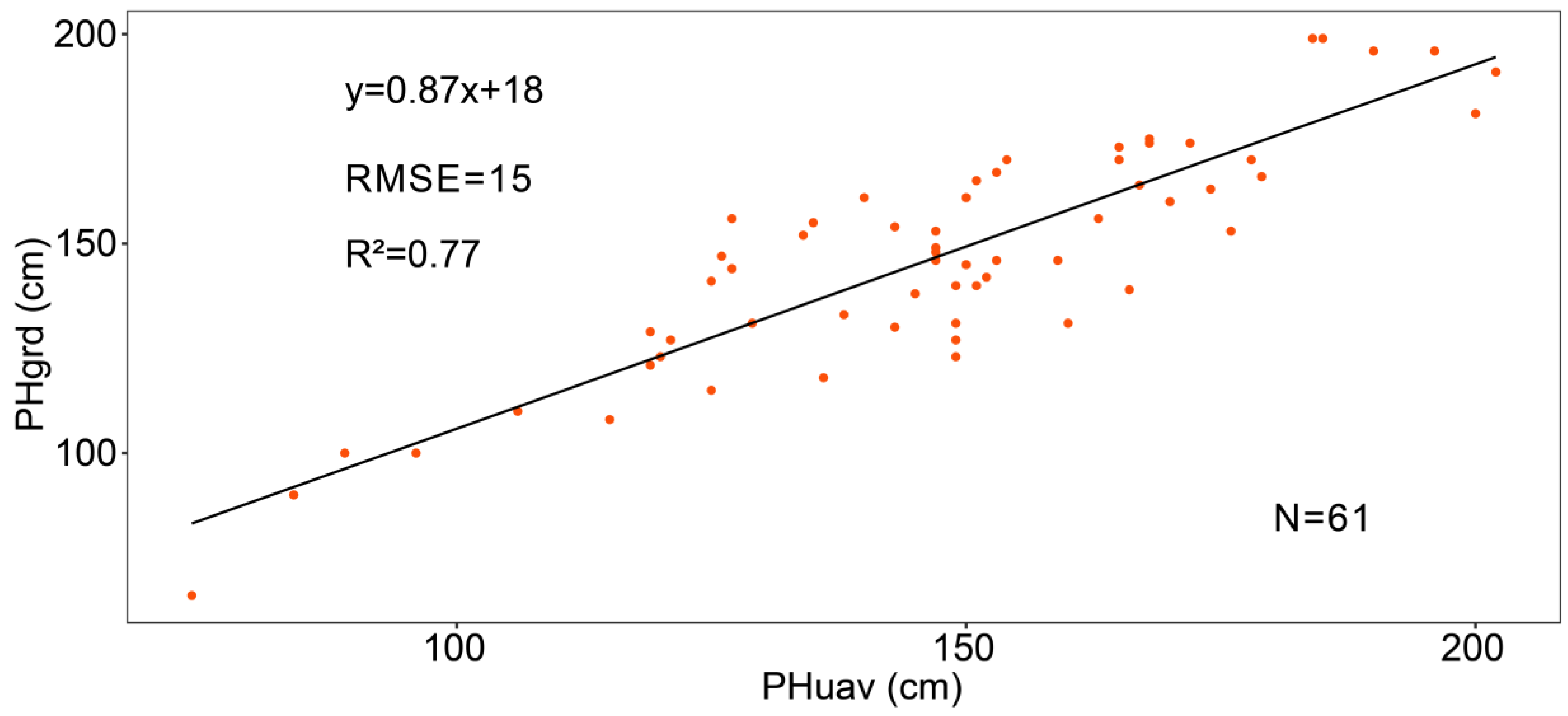
The crop surface model (CSM) was normalized by subtracting the digital elevation model (DEM) from the DSM [29,30]. DSMs were the model output from the Agisoft Photoscan Pro software by using images captured on 8 June and 11 July, respectively. On 8 June, maize was about at growth stage 13 (BBCH-scale) and the average plant height of the plots was less than 20 cm. We extracted 1332 elevation points from the DSM on 8 June that were not covered with vegetation. The DEM was interpolated from these 1332 points with the ordinary Kriging spatial interpolation method by using ArcMap. Using AOIs (only cover vegetation), we extracted plant height information on 11 11 July from the CSM by the ENVI software (version 4.5, Esri Inc., Redlands, CA, USA). A linear fitting model was developed to test the relationship of the plant height between UAV observations and manual measurements. This model explained 77% of the variations in maize plant height, with a root mean square error (RMSE) of 15 cm (Figure 2).

In the stitching processing, 16 GCPs were used to optimize the camera position and orientation, which allowed for the improvement of the georeferenced accuracy of the DSM and orthoimage. The contents listed in

Table 1. Processing quality report for evaluating the accuracy of DSMs and orthoimage.

Date	X Error (cm)	Y Error (cm)	Z Error (cm)	Total Error (cm)	Point Density (points/cm²)
8 June	0.93	1.02	0.49	1.46	47.9
11 July	1.28	1.46	0.73	2.08	13.7

Abbreviation: Error—Root mean square error (RMSE) of the GCPs. X—Longitude, Y—Latitude, Z—Altitude.

were used to evaluate the accuracy of DSMs and orthoimage.

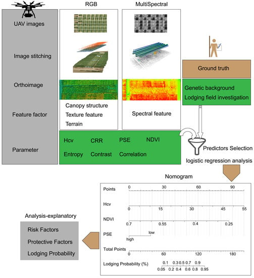
2.3. Potential Factors for Maize Lodging

Before and after the lodging, canopy structure, texture, and spectral characteristics of the maize population changed to varying degrees, which were regarded as feature factors of maize lodging identification in this study. The genetic background was reported to be related to the lodging resistance of maize [31,32], so the genetic background (G) was considered as a potential factor. Although previous studies had shown that planting density had an impact on crop lodging [33], this trial adopted uniform standard mechanized planting, averaging about 24 plants in a plot, so planting density factor was not considered.

Since the plot was small and flat, the surface elevation (PSE) of a plot could be represented by one single numeric value. PSE is an average value calculated by the elevation values at four corners and center of a plot. These elevation values were extracted from the DEM. After multiple rainfalls, terrain may cause spatial variability in the soil moisture, leading to waterlogging in parts of the study area. Therefore, the PSE revealed terrain changes at the plot scale, which was considered a potential factor for lodging identification.

In this study, the canopy structure was described in two dimensions: horizontal and vertical. Canopy cover (CC) was regarded as an indicator of the development of the canopy structure in the horizontal direction, implicating information on maize leaf density and planting area. According to Reference [34], green and non-green pixels in the orthoimage were segmented by using the excess green index (EXG) proposed by Woebbecke et al. [35]. CC was calculated as the ratio of the area between green pixels and total pixels within a plot. Canopy elevation relief ratio (CRR) and the coefficient of variation of canopy height (Hcv) were the metrics of the vertical canopy structure. Hcv is defined as the ratio of the canopy height standard deviation (Hstd) to the mean (Hmean), which has been confirmed by multiple studies to effectively describe the heterogeneity of the canopy plant height in the vertical direction [10,36,37,38]. CRR is commonly used as a metric that describes the relative shape of the canopy in forestry studies, which can be calculated with minimum (Hmin), maximum (Hmax), and mean (Hmean) of the plant height. CRR represents the degree to which the outer canopy surfaces are in the upper (CRR > 0.5) or in the lower (CRR < 0.5) portions of the height range [39,40].

Gray-co-occurrence matrices (GLCM) were frequently used to quantitatively evaluate texture features that can be used for image classification and target recognition [41]. Previous studies had shown no redundancy between Entropy, Contrast, and Correlation in many GLCM textural parameters [42]. Therefore, the three texture feature parameters were considered as potential factors. Minarno et al. [43] had introduced the extraction method of texture feature parameters in detail.

According to Reference [14], the normalized difference vegetation index (NDVI) had a good indication of the lodging identification, where the relative increase of the canopy spectral reflectance in the visible light band was higher than that in the near-infrared band after lodging. Therefore, NDVI as a spectral feature parameter participated in the lodging recognition and factor analysis. Potential feature factors and parameters are summarized in

Table 2. Potential feature factors and parameters.

Feature Categories	Parameter Name	Calculation Formula (or Value)	Parameter Connotation	References
Texture	Entropy	$\mathrm{Entropy}={\displaystyle \sum _{i,j=0}^{N-1}-P_{ij}\ln P_{ij}}$	Measures the amount of information in the image and represents the complexity of the texture.	[41,42]
	Contrast	$\mathrm{Contrast}={\displaystyle \sum _{i,j=0}^{N-1}{P}_{ij}}{(i-j)}^2$	Reflects the total amount of local gray changes in the image
	Correlation	$\mathrm{Correlation}={\displaystyle \sum _{i,j=0}^{N-1}{P}_{ij}\frac{(i-\mu )(j-\mu )}{{\sigma }^2}}$	Describes the degree of similarity between row and column elements in GLCM, and reflects the extension of a grayscale in a direction.
Spectral characteristics	NDVI	$\mathrm{NDVI}=\frac{{\rho }_{nir}-{\rho }_{red}}{{\rho }_{nir}+{\rho }_{red}}$	NDVI is a common vegetation index and data product, and is used to evaluate whether the target being observed contains live green vegetation or not and monitors the vegetation health condition.	[44,45]
Canopy structure	Canopy Cover	$\mathrm{EXG}=2G-R-B$ $\mathrm{CC}=\frac{Are{a}_{greenplants}}{Are{a}_{plot}}$	EXG is a vegetation index that is used for image segmentation. CC reflects the development of the canopy structure in the horizontal direction.	[35,46]
	Hcv	$\mathrm{HCV}=\frac{H_{std}}{H_{mean}}$	One-dimensional metric that describe the vertical heterogeneity of plant canopy height.	[10]
	CRR	$\mathrm{CRR}=\frac{H_{mean}-H_{min}}{H_{max}-H_{min}}$	Three-dimensional metric that describes the horizontal and vertical heterogeneities of plant canopy height.	[38,47]
Terrain	PSE	$\mathrm{PSE}=\frac{E{L}_1+E{L}_2+E{L}_3+E{L}_4+E{L}_5}{5}$	Indicates the elevation at the plot scale
Genetic background	G	G1,G2,G3,G4,G5	Five different genetic backgrounds of maize that have differences in growth period and stalk stiffness.

.

P_ij is element i,j of the normalized symmetrical GLCM. N is the number of gray levels in the image as specified by the number of levels under quantization on the GLCM texture page of the variable properties dialog box. $\mu$ is the GLCM mean, and is calculated using: $\mu ={\displaystyle \sum _{i,j=0}^{N-1}i{P}_{ij}}$. ${\sigma }^2$ is the variance of the intensities of all reference pixels in the relationships that contributed to the GLCM, and is calculated using: ${\sigma }^2={\displaystyle \sum _{i,j=0}^{N-1}{P}_{ij}{\left(i-\mu \right)}^2}$. EXG is the excess green index, NDVI is the normalized difference vegetation index, CC is the canopy cover, and CRR is the canopy elevation relief ratio. $H_{min}$, $H_{\max }$, $H_{mean}$, and $H_{std}$ represent the minimum, maximum, mean, and standard deviation of the plant height at the plot scale, respectively. $Area$ indicates the calculation of areas, and ${\rho }_{nir}$ and ${\rho }_{red}$ are the reflectances for near-infrared and red bands, respectively. $E{L}_i$ represents the elevation at five sampling points of a plot.

These feature parameter acquisitions were repeated for each plot based on the 11 July data and divided into two groups, namely, the lodging group and non-lodging group. We combined a field investigation and image-based visual interpretation to determine the ground truth; namely, whether lodging occurs in a plot. Before and after lodging, the change of stem-to-leaf ratio at the plot scale was the main visual discrimination criterion. Stalks of maize in the lodging plots were clearly observed from the orthoimage (Figure 1C part). The non-lodging group treated as a control group was created using stratified random sampling according to row number. When modeling, CC, CRR, Hcv, NDVI, Entropy, Contrast, and Correlation were treated as continuous variables, and PSE and G were treated as categorical variables. Therefore, PSE needed to be discretized and converted into categorical variables so that it was easier to interpret the results. In this study, the R package “apcluster” (version 1.4.5) [48] was used to implement the affinity propagation (AP) clustering algorithm [49], which could automatically determine the optimal number of clusters. The clustering result was divided into two grades, high and low, which represented the difference in terrain within the study area.

2.4. Predictors Selection and Modeling

Predictors (i.e., feature parameters) should have significant differences between the lodging and non-lodging group. In order to preliminarily filter some potential predictors that were not relevant for modeling, testing for significant differences between the two groups was performed. According to different data distribution conditions (normal or non-normal distribution) and types of predictor variables (continuous or categorical variables), different test methods were used. A Shapiro and Wilk test at the 0.05 level was applied to check whether continuous predictor variables followed a normal distribution [50]. If the continuous predictor variables followed the normal distribution, the mean and standard deviation was used to describe the distribution of predictors, and the t-test was used to compare the difference between groups; otherwise, the median and interquartile was used to describe the distribution of predictors, and a Mann Whitney U test was used to compare the difference between groups. No statistically significant continuous predictor variables (p-value > 0.05) were removed and no longer involved in modeling [51]. A χ² test was applied to check for categorical predictor variables, and no statistically significant categorical predictor variables (p-value > 0.05) were retained [24].

Univariate logistic regression analysis was used to examine whether predictor variables had an independent effect on maize lodging and preliminarily determined predictors relevant for modeling [52]. Multivariate logistic regression analysis was used to further explore confounding predictors and discover the underlying association between the outcome and the selected predictors [53]. Backward selection procedures applying asymptotic significant correlations for the log-likelihood ratio test (p-value < 0.001) were used to select the predictors in the logistic regression analysis.

In this study, the binary logistic regression model was created to estimate the probability of a binary outcome (i.e., non-lodging or lodging) based on multiple selected predictors. Lodging was coded as “1”, and a contrary outcome (i.e., non-lodging) was coded as “0”. Following this, a binary outcome named “Islodging” was defined for modeling:

Islodging = 0, the negative outcome, if a non-lodging event occurred in a plot

Islodging = 1, the positive outcome, if a lodging event occurred in a plot

The probability of a positive outcome is P and that of a negative outcome is Q (Q = 1 − P). Then, the logit for multivariable logistic regression given by the equation below:

$$Logit\left(P\right)={\beta }_0+{\beta }_1{H}_{cv}+{\beta }_{2}NDVI+{\beta }_{3}PSE+\cdot \cdot \cdot$$

(1)

The lodging probability is:

$$P=\frac{EXP\left({\beta }_0+{\beta }_1{H}_{cv}+{\beta }_{2}NDVI+{\beta }_{3}PSE+\cdot \cdot \cdot \right)}{1+EXP\left({\beta }_0+{\beta }_1{H}_{cv}+{\beta }_{2}NDVI+{\beta }_{3}PSE+\cdot \cdot \cdot \right)}$$

(2)

where ${\beta }_0$ is the intercept, ${\beta }_i$ are regression coefficients, and Hcv, NDVI, PSE, and so on are the predictors. ${\beta }_0$ and ${\beta }_i$ were estimated using the maximum likelihood method, which is designed to maximize the likelihood of reproducing the data given the parameter estimates [54]. A Hosmer–Lemeshow test (p-value > 0.05 indicating good fit) was performed to test the fitting degree of logistic regression model and to ensure that all the factors in the model were adequately utilized [55].

The ratio of P to Q is defined as the odds ratio (OR). The outcome of a logistic regression model is the logarithm of the OR, which is linearly related to the weighted sum of multiple predictors. The odds ratios and 95% confidence intervals (CI) were calculated. The interpretation of final logistic regression model for maize lodging was rendered using the OR-value of predictors. When ${\beta }_i$ > 0 and OR > 1 in the models, the predictor variable was deemed as a risk factor. When ${\beta }_i$ < 0 and OR < 1 in the models, the predictor variable was deemed as a protective factor [56,57].

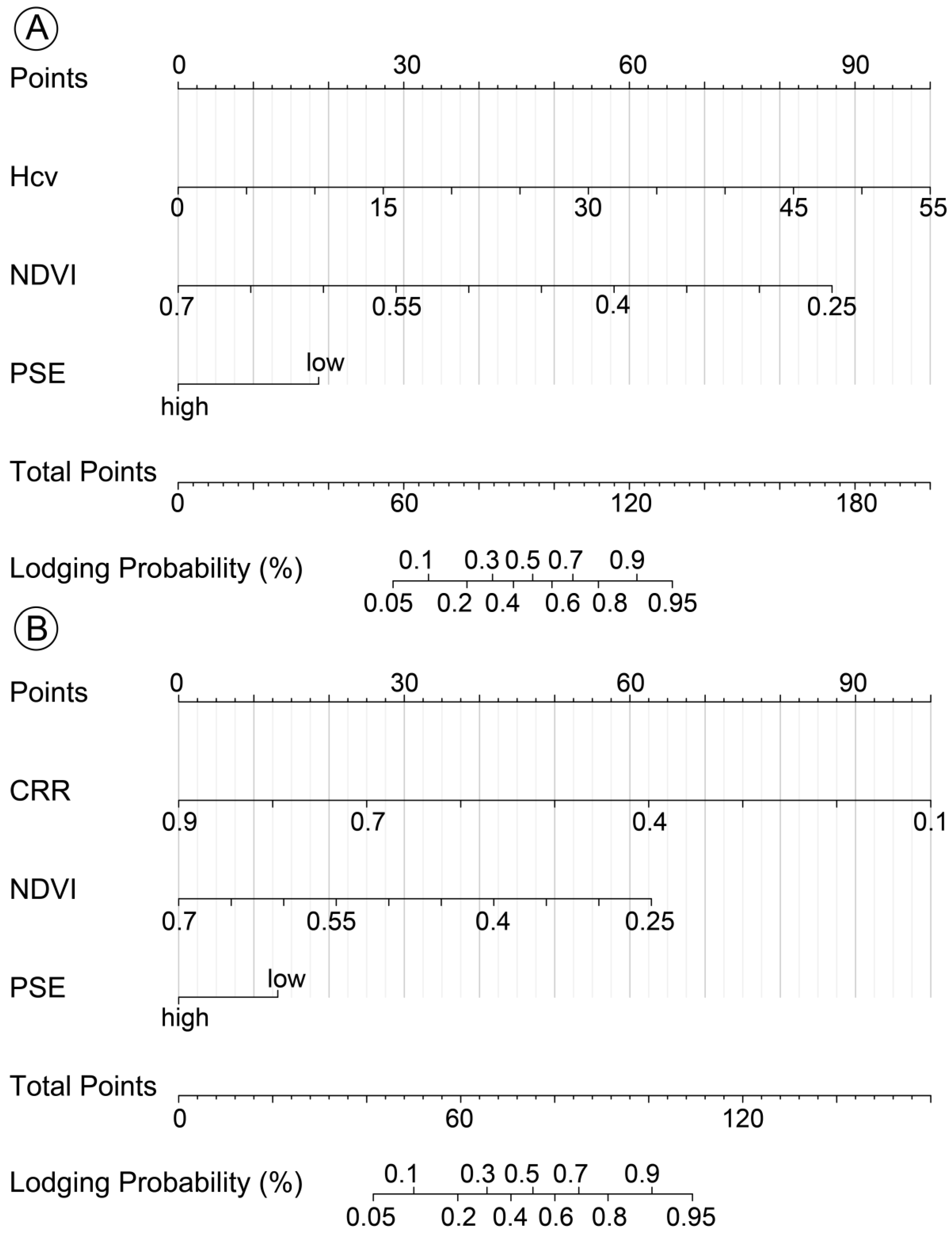
2.5. Nomogram Construction and Evaluation

Nomograms were constructed to evaluate the lodging probability and the strength effect of each predictor. In the nomogram, the point corresponding to a predictor variable was converted from the fitting coefficient of the regression model. The predictor with the largest strength effect on lodging was taken as the reference and all points were rescaled to values between 0 and 100 [25]. Longer horizontal lines represent larger points and indicate the larger effects on lodging. Total points at the bottom scale provided insight into the likelihood that a maize plot will be lodging.

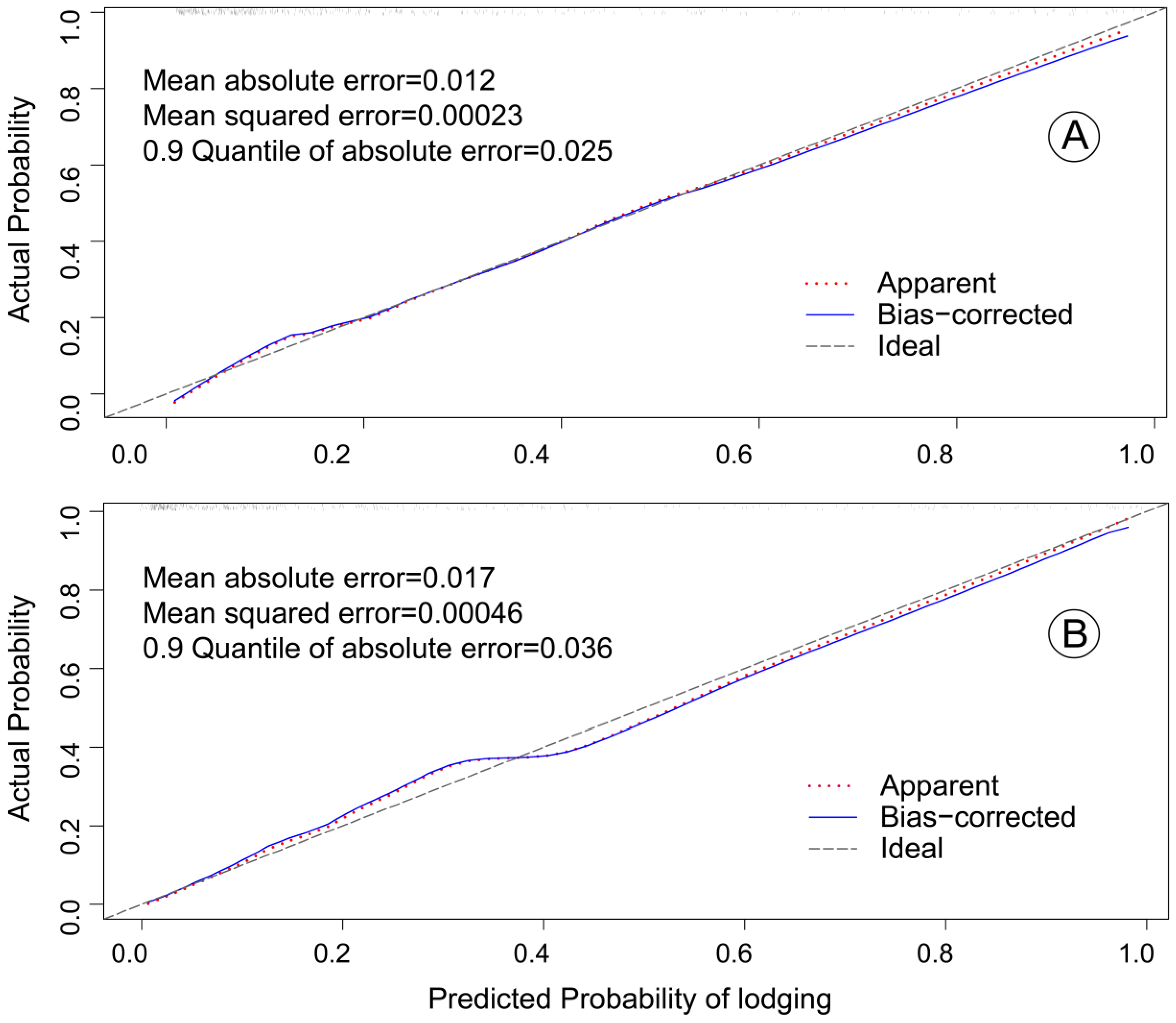
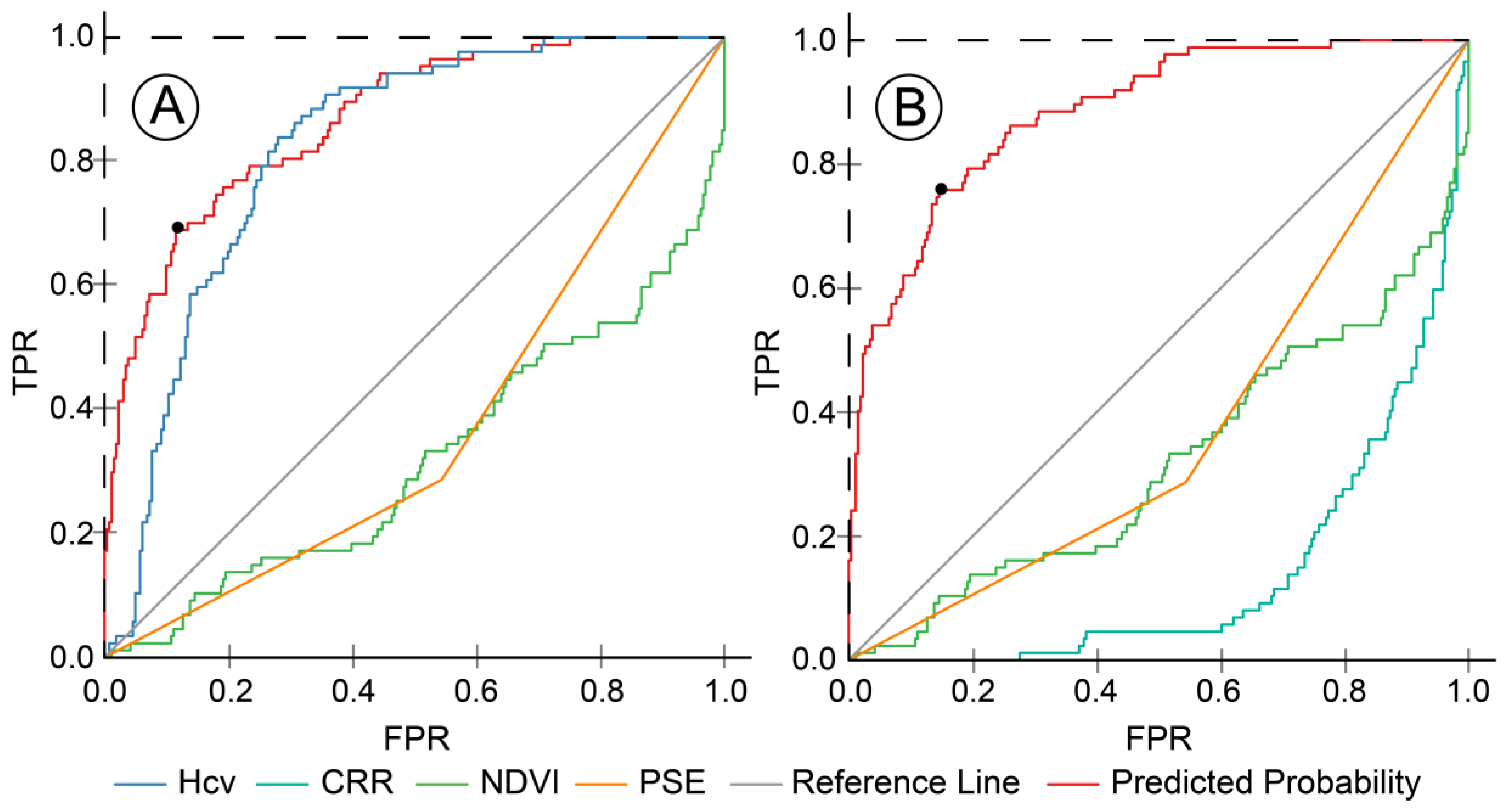
The effectiveness evaluation of the model included two indicators, namely discrimination and calibration, which were performed by the area under receiver operating characteristic (ROC) curve and a calibration method, respectively [58]. The true positive rate (TPR) and false positive rate (FPR) are the vertical axis and horizontal axis of the ROC, respectively. TPR, also known as sensitivity, referred to the percentage that an actual lodging was correctly judged as lodging. FPR, also known as (1 − specificity), referred to the percentage that non-lodging was incorrectly judged as lodging. The area under the ROC curve (AUC) was developed as a discrimination criterion. According to Hosmer and Lemeshow, AUC = 0.5 corresponds to randomly guess and AUC > 0.7 corresponds to a reasonable recognition [59,60]. Calibration measures the model’s ability to generate predictions that are on average closer to the average observed outcome, which is used to validate the robustness of the models [61]. A visual calibration plot was used to illustrate the correlation between the actual probability and the predicted probability by a bootstrapping method [24,62].

Youden’s J statistic is another main summary statistic of the ROC curve used interpret and evaluate the performance of the model [63], which ranged between 0 and 1, with values close to 1 indicating that the model’s effectiveness was relatively large and values close to 0 indicating limited effectiveness [64]. The maximum value of the Youden’s J statistic was used as a criterion for selecting the optimum cutoff point [65]. J is defined as J = sensitivity + specificity − 1 [66].

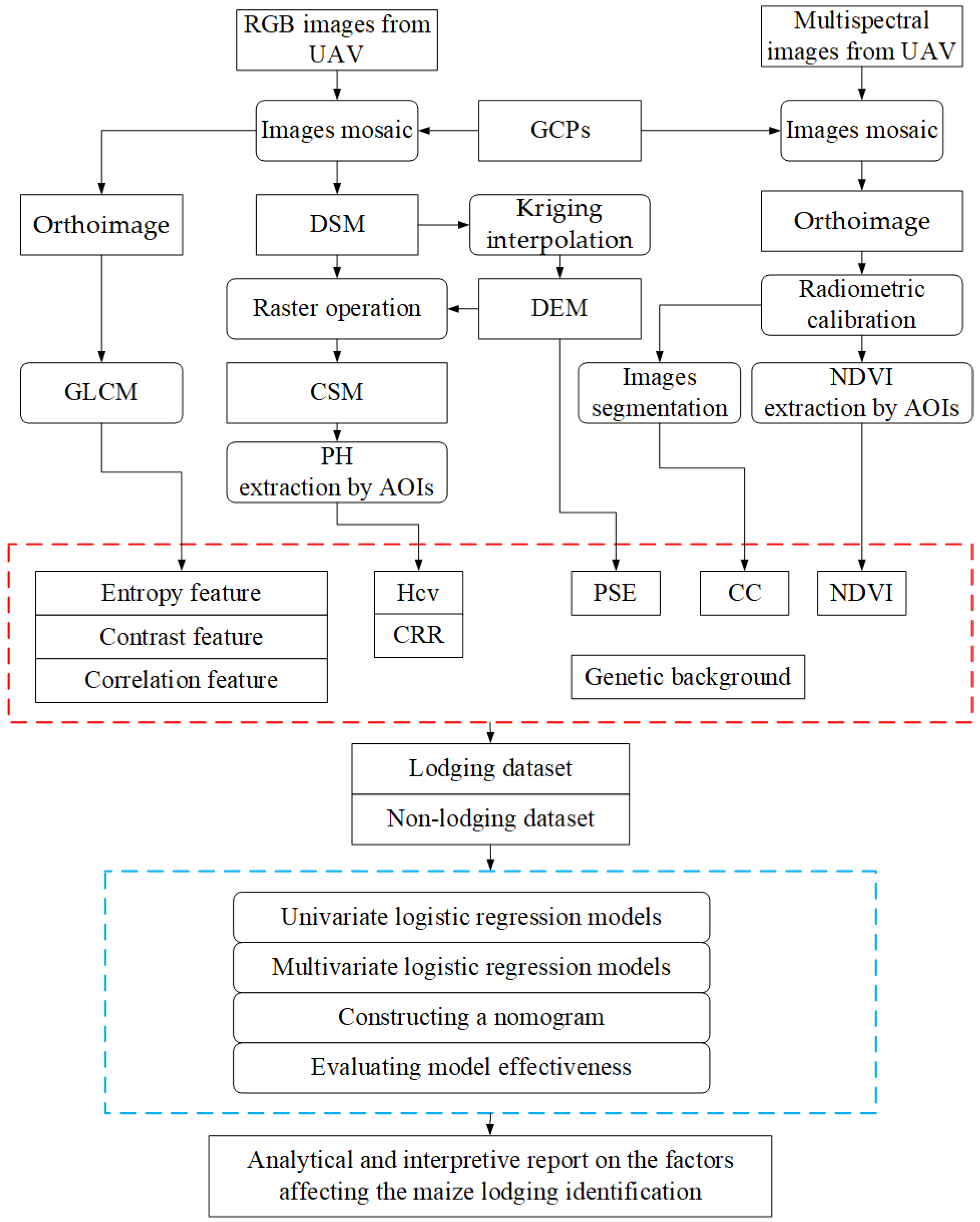
Statistical analysis, modeling, and evaluation were carried out using an R software version 3.4.3 for Windows (https://www.r-project.org) with R packages (apcluster, ggplot2, rms, and pROC). The schematic diagram of data processing and analysis procedure for maize lodging recognition is illustrated in Figure 3.

3. Results and Analysis

3.1. Comparisons on Data Distribution

Among the 348 plots included in this study, 87 lodging plots were observed. Figure 4 shows data distribution characteristics of continuous predictor variables extracted from UAV images. There were statistically significant differences in CC, NDVI, Hcv, CRR, PSE, G, and Correlation between the lodging and non-lodging groups. Contrast and Entropy as textural feature parameters were not significantly different between the two groups (p-value > 0.05), which were removed from the model. Correlation was a measure of the similarity between elements of GLCM in a row or column direction, revealing the change in the extension direction of the image texture before and after lodging, which may be affected by the appearance of maize stalks in the images. The difference of CRR and Hcv between the two groups reached a very significant level (p-value < 0.001). This revealed that the changes in canopy structure (plant height) was the most obvious before and after lodging. The difference between non-lodging and lodging groups are summarized in

Table 3. Difference between non-lodging and lodging groups. The table shows the statistical description of predictors in the two groups. p-Value is used to indicate whether the predictors have statistically significant differences in the two groups.

Variables (Factors)	Non-Lodging Group (n = 261)	Lodging Group (n = 87)	p-Value
CC $\left[\mathrm{M}\left(\mathrm{Q}1,\mathrm{Q}3\right)\right]$	0.604 (0.520,0.661)	0.661 (0.539,0.744)	0.03
NDVI $\left[\mathrm{M}\left(\mathrm{Q}1,\mathrm{Q}3\right)\right]$	0.556 (0.508,0.585)	0.515 (0.430,0.561)	0.02
Hcv $\left[\mathrm{M}\left(\mathrm{Q}1,\mathrm{Q}3\right)\right]$	12.943 (10.449,19.213)	23.841 (19.823,29.681)	0.000
CRR $\left[\mathrm{M}\left(\mathrm{Q}1,\mathrm{Q}3\right)\right]$	0.747 (0.684,0.798)	0.565 (0.469,0.663)	0.000
PSE (m), level, n%			0.157
low	119 (31.3%)	62 (17.8%)	l
high	142 (24.4%)	25 (1.7%)
G, group, n%			0.220
G1	79 (22.7%)	4 (1.1%)
G2	33 (9.6%)	17 (4.8%)
G3	38 (10.9%)	23 (6.6%)
G4	13 (3.7%)	2 (0.6%)
G5	98 (28.2%)	41 (11.8%)
Contrast $\left(\overline{x}\pm s\right)$	5.473 (1.123)	0.664 (0.039)	0.718
Entropy $\left[\mathrm{M}\left(\mathrm{Q}1,\mathrm{Q}3\right)\right]$	1.987 (1.966,2.011)	1.994 (1.961,2.014)	0.568
Correlation $\left(\overline{x}\pm s\right)$	0.659 (0.040)	0.664 (0.039)	0.02

Abbreviations: $\overline{x}$ = mean, $s$ = standard deviation, M = median, Q1 and Q3 = interquartile range.

.

The results of the Pearson’s correlation coefficient ($\mathsf{\rho }=-0.638$) indicated that CRR was correlated negatively and significantly with Hcv. Therefore, they were not suitable for predictors in the same model. Replacing Hcv in Equations (4) and (5) with CRR, two different logistic regression analysis models were created, which were called Model-1 and Model-2, respectively.

3.2. Predictors Selection for Maize Lodging

A univariate logistic regression was performed to analyze the association between the lodging of maize and CC, NDVI, Hcv, CRR, PSE, G, and Correlation (

Table 4. Effects of factors on maize lodging by univariate logistic regression analysis.

	OR	95% CI	p-Value
CC	18.51	1.30–263.10	0.031
NDVI	0.000	0.000–0.001	<0.001
Hcv	1.112	1.079–1.146	<0.001
CRR	0.000	0.000–0.001	<0.001
PSE			<0.001
high		1
low	2.959	1.752–4.999	<0.001
G			<0.001
G1		1
G2	10.174	3.182–32.536	<0.001
G3	11.954	3.861–37.009	<0.001
G4	3.038	0.504–18.306	0.225
G5	8.263	8.263–24.055	<0.001
Correlation	3706.100	3.161–4,339,512.425	0.023

Abbreviations: OR = odds ratio. CI = confidence interval of OR.

). NDVI, Hcv, CRR, PSE, and G were selected as preliminary predictors (p-value <0.001). Both NDVI and CRR were continuous predictor variables. The OR-value of NDVI (OR: 0.000, 95% CI: 0.000–0.001) and CRR (OR: 0.000, 95% CI: 0.000–0.001) were the change of logit (P) when they changed every unit respectively, resulting in a very small OR-value. Categorical predictor variable PSEs were all statistically significant in the two models. When adjusting for possible confounders, Hcv, CRR, NDVI, and PSE were still associated with lodging in Model-1 and Model-2, respectively (

Table 5. Multivariable logistic regression analysis of candidate variables (p < 0.001 in univariate logistic regression analysis).

		β	OR	95% CI	p-Value
Model-1	Hcv	0.144	1.155	1.113–1.199	0.000
	NDVI	−15.320	0.000	0.000–0.001	0.000
	PSE	1.482			0.000
	high		1
	low		4.401	2.219–8.728	0.000
	Constant	3.248
Model-2	CRR	−10.842	0.000	0.000–0.001	0.000
	NDVI	−12.115	0.000	0.000–0.001	0.000
	PSE	1.143			0.000
	high		1
	low		3.137	1.584–6.213	0.000
	Constant	11.702

Abbreviations: OR = odds ratio. CI = confidence interval of OR. β and Constant are the coefficients and constant of the final multivariate regression equation, respectively.

). However, G was statistically significant in Model-1 but not in Model-2 at the 0.05 level. We found that G1 only was planted at high altitudes (PSE = high) using a crosstab statistical analysis (

Table 6. Crosstab statistical analysis.

Islodging			G
			1	2	3	4	5	Total
0	PSE	low	0	19	24	11	65	119
		high	79	14	14	2	33	142
	Total		79	33	38	13	98	261
1	PSE	low	0	13	14	1	34	62
		high	4	4	9	1	7	25
	Total		4	17	23	2	41	87

Abbreviations: G = Genetic background. Islodging of 0 represents non-lodging and 1 represents lodging. Low and high are the PSE level.

). This proved that G was associated with PSE. Therefore, G could not be used as an independent predictor variable in the final logistic regression models.

3.3. Construction and Validation of Models

The p-value for the Hosmer–Lemeshow test of Model-1 and Model-2 were 0.735 and 0.736, respectively, indicating a good model fit. The calibration of the two models was performed using two calibration plots with bootstrap resampling 1000 times. Statistical error indicators of Model-1 and Model-2 in the calibration plot illustrated that the two nomograms were well calibrated (Figure 5), and Model-1 had a better calibration result than Model-2. This result showed that the robustness of Model-1 was better than that of Model-2. The AUC of Model-1 and Model-2 were 0.866 (95% CI: 0.824–0.909) and 0.884 (95% CI: 0.844–0.923), respectively (Figure 6). This result showed that the discrimination of Model-2 was better than that of Model-1, which may be due to the fact that CRR describes the three-dimensional canopy structure of maize, while Hcv describes the two-dimensional canopy structure. Compared with univariate regression analysis, multivariate regression analysis can effectively improve the ability of the lodging identification. In rare events, the discrimination of the multivariate regression analysis was worse (e.g., predicted probability line and Hcv line intersected in Figure 6A part). By checking the ROC curve data, these rare events occurred in some data with a fuzzy state, where the non-lodging plots had relatively lower NDVI. However, in most events, non-lodging plots had a higher NDVI.

When Youden’s J statistic reached its maximum value, the cutoff point was farthest from the reference line (Figure 6). In this study, when the optimal cutoff value of the Model-1 was 0.575, TPR and FPR were 69.0% and 11.5%, respectively. When the optimal cutoff value of the Model-2 was 0.613, TPR and FPR were 75.9% and 14.6%, respectively. Youden’s J statistic can also draw the conclusion that Model-2 was superior to Model-1 in term of its discrimination ability.

3.4. Analytical and Interpretive Report

After validating the model effectiveness, this section focuses on the relationship between the outcomes and selected predictors. In Figure 7, the longer horizontal line of Hcv and CRR indicated larger effects on lodging in Model-1 and Model-2, respectively. This showed that the canopy structure was the most important factor affecting lodging identification in this study, which indirectly confirmed the hypothesis proposed in Reference [10] that lodging severity was directly associated with a canopy structural anomaly. The shorter line of NDVI and PSE indicated a relatively marginal role played by NDVI and PSE. The smaller the value of NDVI (β: −12.115, OR: 0.000, 95% CI: 0.000–0.001) and CRR (β: −10.842, OR: 0.000, 95% CI: 0.000–0.001) and the greater the points they have, mean that NDVI and CRR were considered protective factors. The greater the value of Hcv (β: 0.144, OR: 1.155, 95% CI: 1.113–1.199) and the greater the points it has, mean that Hcv was considered a risk factor. The OR-value of PSE at high altitude was taken as a reference (OR-value = 1). The probability of lodging at low altitude was approximately 4.4 times than that at high altitude (Table 5). The terrain map in Figure 1D also qualitatively confirmed this conclusion.

To demonstrate the application of the nomogram (Figure 7), the data of a plot were randomly sampled as an example. The NDVI, Hcv, and CRR of this plot were 0.561, 16.708, and 0.801, respectively. This plot was located at low altitude. Each predictor point and the total points are illustrated in

Table 7. Example of nomogram application.

	Hcv (Points)	CRR (Points)	NDVI (Points)	PSE (Points)	Total Points	Lodging Probability
Model-1	28	—	26	18	72	15%
Model-2	—	12	22	14	48	10%

. According to the nomogram, its probability of lodging was approximately 15% (Model-1) and 10% (Model-2), respectively. It had a 90% probability of inferring that a plot was non-lodging based on the result of Model-2.

4. Discussion

4.1. Sample Size

The failure to give the severity of the lodging was a shortcoming in this paper, which was the result of the sample size limit. Manual grading based on field investigation leads to extreme imbalance of the lodging samples. Manual grading was divided into two levels, namely stalk breakage and root lodging [67]. More than 80% was root lodging. For the three outcomes (i.e., stalk breakage, root lodging, and non-lodging), the sample size of the stalk breakage did not meet the sample size requirements of a multinomial logistic regression. The sample size estimation of logistic regression was influenced by the number and type of predictor variables, and the number of outcomes. The widely accepted principle is that the number of events should be at least 10 times that of the number of predictors in term of each outcome [68]. The differential significance test was used to initially screen for predictors. Then, based on the results of a univariate analysis, statistically significant predictor variables were selected for multivariate logistic analysis. The statistical significance level was set to 0.001. The smaller the value, the stricter the criterion for selecting the predictor variables. The main purpose of taking these steps as above was to limit the number of predictor variables. Aiming at the problem that the proportion of positive samples (lodging samples) was too low, the undersampling method (reducing the number of negative samples) was adopted to increase the proportion of positive samples. It should be noted that the undersampled sample is a biased sample. Theoretically, it can be proved that if the biased sample is used for parameter estimation, only the intercept value of the logistic regression model will be affected, and other parameters are still reliable. Calibration of model parameters that are estimated based on special sampling does not affect the evaluation of model [69]. Therefore, in order to ensure the complete presentation of a positive sample feature, all 87 positive samples were used for modeling in this study. Considering that the outcome of stalk breakage was insufficient, a binary logistic regression model (two outcomes) was created in this study. After stalk breakage samples meet the requirement of modeling, a multinomial logistic regression will be created, which can directly use lodging severity as an outcome.

4.2. Limitations and Implications of this Study

Fewer lodging types and smaller sampling area may be the main reasons for the failure of textural parameters and CC in the differential significance test and univariate logistic analysis, respectively. Figure 6 showed that the curve representing NDVI had a higher volatility, which was related to the data quality. The quality of NDVI was not only affected by the observation conditions, but also related to leaf color, while leaf color was controlled by the environment and genotype interactions [70]. In this study, the lodging of maize had characteristics of contingency. The interaction between the genetic background and the terrain factors was not taken into account at the beginning of the trial design, which led to the genetic background factor not being selected during modeling, while in other studies this factor was considered [31,71]. PSE was a transmission factor. The roots of maize planted at low altitude had more moisture than at high altitude, so they had shallower roots and were more prone to lodging when natural disasters hit. During modeling, the interaction terms were not included. Actually, a logistic regression model also requires predictor variables to be independent. When there are interactions between predictors, the interpretation of the logistic regression coefficient and OR-value become more complex, so special care should be taken.

In this study, only one spectral index (i.e., NDVI) was used. If the UAV platform is equipped with a hyperspectral sensor, there will be more spectral indices to choose from. Compared with a digital camera, point clouds produced by airborne laser scanning (ALS) can more fully characterize the canopy structural complexity of maize [38], which will improve the ability of the model to identify maize lodging. After lodging, the breeders usually help to straighten the lodging maize. Maize stalk is able to maintain its upward growth due to its negative geotropism. The capacity of UAV remote sensing to scale phenotyping up from a few to thousands of breeding plots allows breeders to effortlessly monitor the growth of different breeding varieties after straightening in order to find lodging-resistant breeding varieties.

5. Summary and Conclusions

In this study, multispectral and digital images collected by a UAV system were applied to quantitatively identify feature factors that cause maize lodging. The workflow in this study was suitable to extract and analyze phenotypic traits of a large breeding and agronomy trials. Statistical methods were used to screen several potential predictors and construct two nomograms with better validation performance based on selected predictor factors. Our study could not only find risk factors and protective factors related to the lodging of maize, but also predict the probability of lodging under different predictor variables. Due to the lack of data validation for multiple growth stages, although prediction ability of these models is available, the stability of prediction needs further study. Among many factors, the canopy structure is the main-effect factor, and spectral characteristics and terrain factors are secondary. The reminder given to us is that when screening maize lodging-resistant varieties, we should pay enough attention to the problem of spatial variability in the terrain.

References

1. National Bureau of Statistics of China. Announcement on Grain Production in 2017. Available online: http://www.stats.gov.cn/tjsj/zxfb/201712/t20171208_1561546.html (accessed on 11 May 2018).
2. Murakami, T.; Yui, M.; Amaha, K. Canopy height measurement by photogrammetric analysis of aerial images: Application to buckwheat (Fagopyrum esculentum Moench) lodging evaluation. Comput. Electron. Agric. 2012, 89, 70–75. [Google Scholar] [CrossRef]
3. Pinthus, M.J. Lodging in wheat, barley, and oats: The phenomenon, its causes, and preventive measures. Adv. Agron. 1974, 25, 209–263. [Google Scholar]
4. Tumino, G.; Voorrips, R.E.; Morcia, C.; Ghizzoni, R.; Germeier, C.U.; Paulo, M.J.; Terzi, V.; Smulders, M.J.M. Genome-wide association analysis for lodging tolerance and plant height in a diverse European hexaploid oat collection. Euphytica 2017, 213, 163. [Google Scholar] [CrossRef]
5. Shakoor, N.; Lee, S.; Mockler, T.C. High throughput phenotyping to accelerate crop breeding and monitoring of diseases in the field. Curr. Opin. Plant Boil. 2017, 38, 184–192. [Google Scholar] [CrossRef] [PubMed]
6. Liu, T.; Li, R.; Zhong, X.; Jiang, M.; Jin, X.; Zhou, P.; Liu, S.; Sun, C.; Guo, W. Estimates of rice lodging using indices derived from UAV visible and thermal infrared images. Agric. For. Meteorol. 2018, 252, 144–154. [Google Scholar] [CrossRef]
7. Hu, P.; Chapman, S.C.; Wang, X.; Potgieter, A.; Duan, T.; Jordan, D.; Guo, Y.; Zheng, B. Estimation of plant height using a high throughput phenotyping platform based on unmanned aerial vehicle and self-calibration: Example for sorghum breeding. Eur. J. Agron. 2018, 95, 24–32. [Google Scholar] [CrossRef]
8. Duan, T.; Chapman, S.C.; Guo, Y.; Zheng, B. Dynamic monitoring of NDVI in wheat agronomy and breeding trials using an unmanned aerial vehicle. Field Crop. Res. 2017, 210, 71–80. [Google Scholar] [CrossRef]
9. Han, D.; Yang, H.; Yang, G.; Qiu, C. Monitoring model of maize lodging based on sentinel-1 radar image. Trans. Chin. Soc. Agric. Eng. 2018, 34, 166–172. [Google Scholar]
10. Chu, T.X.; Starek, M.J.; Brewer, M.J.; Murray, S.C.; Pruter, L.S. Assessing lodging severity over an experimental maize (Zea mays L.) field using UAS images. Remote Sens. 2017, 9, 923. [Google Scholar] [CrossRef]
11. Li, Z.; Chen, Z.; Wang, L.; Liu, J.; Zhou, Q. Area extraction of maize lodging based on remote sensing by small unmanned aerial vehicle. Nongye Gongcheng Xuebao 2014, 30, 207–213. [Google Scholar]
12. Matese, A.; Toscano, P.; Di Gennaro, S.; Genesio, L.; Vaccari, F.; Primicerio, J.; Belli, C.; Zaldei, A.; Bianconi, R.; Gioli, B. Intercomparison of UAV, aircraft and satellite remote sensing platforms for precision viticulture. Remote Sens. 2015, 7, 2971–2990. [Google Scholar] [CrossRef]
13. Yang, H.; Chen, E.; Li, Z.; Zhao, C.; Yang, G.; Pignatti, S.; Casa, R.; Zhao, L. Wheat lodging monitoring using polarimetric index from radarsat-2 data. Int. J. Appl. Earth Obs. Geoinf. 2015, 34, 157–166. [Google Scholar] [CrossRef]
14. Liu, L.Y.; Wang, J.H.; Song, X.Y.; Chun-Jun, L.I.; Huang, W.J.; Zhao, C.J. The canopy spectral features and remote sensing of wheat lodging. J. Remote Sens. 2005, 9, 323. [Google Scholar]
15. Li, Z.; Chen, Z.; Ren, G.; Li, Z.; Wang, X. Estimation of maize lodging area based on worldview-2 image. Trans. Chin. Soc. Agric. Eng. 2016, 32, 1–5. [Google Scholar]
16. Liu, H.; Yang, G.-J.; Zhu, H.C. The extraction of wheat lodging area in UAV’S image used spectral and texture features. Appl. Mech. Mater. 2014, 651–653, 2390–2393. [Google Scholar] [CrossRef]
17. Yang, M.D.; Huang, K.S.; Kuo, Y.H.; Tsai, H.P.; Lin, L.M. Spatial and spectral hybrid image classification for rice lodging assessment through UAV imagery. Remote Sens. 2017, 9, 583. [Google Scholar] [CrossRef]
18. Navabi, A.; Iqbal, M.; Strenzke, K.; Spaner, D. The relationship between lodging and plant height in a diverse wheat population. Can. J. Plant Sci. 2006, 86, 723–726. [Google Scholar] [CrossRef] [Green Version]
19. Cox, D.R. The regression analysis of binary sequences. J. R. Stat. Soc. Ser. B (Methodol.) 1958, 20, 215–242. [Google Scholar]
20. Freedman, D.A. Statistical Models: Theory and Practice; Cambridge University Press: Cambridge, UK, 2009. [Google Scholar]
21. Mohammedkhair, A.A.; Hamdi, A.M.A.; Qurashi, M. Comparison between logistic and calibration linear regression. IOSR J. Math. 2016, 12, 125–130. [Google Scholar] [CrossRef]
22. Dreiseitl, S.; Harbauer, A.; Binder, M.; Kittler, H. Nomographic representation of logistic regression models: A case study using patient self-assessment data. J. Biomed. Inform. 2005, 38, 389–394. [Google Scholar] [CrossRef] [PubMed]
23. Wang, Y.; Li, J.; Xia, Y.; Gong, R.; Wang, K.; Yan, Z.; Wan, X.; Liu, G.; Wu, D.; Shi, L.; et al. Prognostic nomogram for intrahepatic cholangiocarcinoma after partial hepatectomy. J. Clin. Oncol. 2013, 31, 1188–1195. [Google Scholar] [CrossRef] [PubMed]
24. Jin, X.; Jiang, Y.Z.; Chen, S.; Yu, K.D.; Ma, D.; Sun, W.; Shao, Z.M.; Di, G.H. A nomogram for predicting pathological complete response in patients with human epidermal growth factor receptor 2 negative breast cancer. BMC Cancer 2016, 16, 606. [Google Scholar] [CrossRef] [PubMed]
25. Bertens, L.C.M.; Moons, K.G.M.; Rutten, F.H.; van Mourik, Y.; Hoes, A.W.; Reitsma, J.B. A nomogram was developed to enhance the use of multinomial logistic regression modeling in diagnostic research. J. Clin. Epidemiol. 2016, 71, 51–57. [Google Scholar] [CrossRef] [PubMed]
26. Lancashire, P.D.; Bleiholder, H.; Boom, T.V.D.; Langelüddeke, P.; Stauss, R.; Weber, E.; Witzenberger, A. A uniform decimal code for growth stages of crops and weeds. Ann. Appl. Boil. 1991, 119, 561–601. [Google Scholar] [CrossRef]
27. Haghighattalab, A.; Perez, L.G.; Mondal, S.; Singh, D.; Schinstock, D.; Rutkoski, J.; Ortiz-Monasterio, I.; Singh, R.P.; Goodin, D.; Poland, J. Application of unmanned aerial systems for high throughput phenotyping of large wheat breeding nurseries. Plant Methods 2016, 12, 35. [Google Scholar] [CrossRef] [PubMed]
28. Otsu, N. A threshold selection method from gray-level histograms. IEEE Trans. Syst. Man Cybern. 1979, 9, 62–66. [Google Scholar] [CrossRef]
29. Holman, F.H.; Riche, A.B.; Michalski, A.; Castle, M.; Wooster, M.J.; Hawkesford, M.J. High throughput field phenotyping of wheat plant height and growth rate in field plot trials using UAV based remote sensing. Remote Sens. 2016, 8, 1031. [Google Scholar] [CrossRef]
30. Bendig, J.; Yu, K.; Aasen, H.; Bolten, A.; Bennertz, S.; Broscheit, J.; Gnyp, M.L.; Bareth, G. Combining UAV-based plant height from crop surface models, visible, and near infrared vegetation indices for biomass monitoring in barley. Int. J. Appl. Earth Obs. Geoinf. 2015, 39, 79–87. [Google Scholar] [CrossRef]
31. Larsson, S.J.; Peiffer, J.A.; Edwards, J.W.; Ersoz, E.S.; Flint-Garcia, S.A.; Holland, J.B.; McMullen, M.D.; Tuinstra, M.R.; Romay, C.; Buckler, E.S. Genetic analysis of lodging in diverse maize hybrids. bioRxiv 2017. [Google Scholar] [CrossRef]
32. Peiffer, J.A.; Flint-Garcia, S.A.; De Leon, N.; McMullen, M.D.; Kaeppler, S.M.; Buckler, E.S. The genetic architecture of maize stalk strength. PLoS ONE 2013, 8, e67066. [Google Scholar] [CrossRef] [PubMed]
33. Xue, J.; Xie, R.Z.; Zhang, W.F.; Wang, K.R.; Hou, P.; Ming, B.; Gou, L.; Li, S.K. Research progress on reduced lodging of high-yield and -density maize. J. Integr. Agric. 2017, 16, 2717–2725. [Google Scholar] [CrossRef]
34. Joalland, S.; Screpanti, C.; Gaume, A.; Walter, A. Belowground biomass accumulation assessed by digital image based leaf area detection. Plant Soil 2016, 398, 257–266. [Google Scholar] [CrossRef]
35. Woebbecke, D.M.; Meyer, G.E.; Bargen, K.V.; Mortensen, D.A. Color indices for weed identification under various soil, residue, and lighting conditions. Trans of the ASAE 1995, 38, 259–269. [Google Scholar] [CrossRef]
36. Næsset, E.; Bjerknes, K.O. Estimating tree heights and number of stems in young forest stands using airborne laser scanner data. Remote Sens. Environ. 2001, 78, 328–340. [Google Scholar] [CrossRef]
37. Li, W.; Niu, Z.; Huang, N.; Wang, C.; Gao, S.; Wu, C.Y. Airborne lidar technique for estimating biomass components of maize: A case study in Zhangye city, northwest China. Ecol. Indic. 2015, 57, 486–496. [Google Scholar] [CrossRef]
38. Li, W.; Niu, Z.; Chen, H.; Li, D. Characterizing canopy structural complexity for the estimation of maize LAI based on ALS data and UAV stereo images. Int. J. Remote Sens. 2017, 38, 2106–2116. [Google Scholar] [CrossRef]
39. Pike, R.J.; Wilson, S.E. Elevation-relief ratio, hypsometric integral, and geomorphic area-altitude analysis. Geol. Soc. Am. Bull. 1971, 82, 1079–1084. [Google Scholar]
40. Parker, G.G.; Russ, M.E. The canopy surface and stand development: Assessing forest canopy structure and complexity with near-surface altimetry. For. Ecol. Manag. 2004, 189, 307–315. [Google Scholar] [CrossRef]
41. Soh, L.K.; Tsatsoulis, C. Texture analysis of SAR sea ice imagery using gray level co-occurrence matrices. IEEE Trans. Geosci. Remote Sens. 1999, 37, 780–795. [Google Scholar] [CrossRef] [Green Version]
42. Bo, H.; Ma, F.L.; Jiao, L.C. Research on computation of GLCM of image texture. Acta Electron. Sin. 2006, 1, 155–158. [Google Scholar]
43. Minarno, A.E.; Munarko, Y.; Kurniawardhani, A.; Bimantoro, F.; Suciati, N. Texture feature extraction using co-occurrence matrices of sub-band image for batik image classification. In Proceedings of the International Conference on Information and Communication Technology, Bandung, Indonesia, 28–30 May 2014; pp. 249–254. [Google Scholar]
44. Tucker, C.J. Red and photographic infrared linear combinations for monitoring vegetation. Remote Sens. Environ. 1979, 8, 127–150. [Google Scholar] [CrossRef] [Green Version]
45. Rouse, J.W., Jr.; Haas, R.H.; Schell, J.A.; Deering, D.W. Monitoring vegetation systems in the great plains with erts. In Third Earth Resources Technology Satellite-1 Symposium; Freden, S.C., Mercanti, E.P., Becker, M.A., Eds.; NASA: Washington, DC, USA, 1974; Volume 1, pp. 309–317. [Google Scholar]
46. Duan, T.; Zheng, B.Y.; Guo, W.; Ninomiya, S.; Guo, Y.; Chapman, S.C. Comparison of ground cover estimates from experiment plots in cotton, sorghum and sugarcane based on images and ortho-mosaics captured by UAV. Funct. Plant Boil. 2017, 44, 169–183. [Google Scholar] [CrossRef]
47. Parker, G.G.; Harmon, M.E.; Lefsky, M.A.; Chen, J.Q.; Van Pelt, R.; Weis, S.B.; Thomas, S.C.; Winner, W.E.; Shaw, D.C.; Frankling, J.F. Three-dimensional structure of an old-growth Pseudotsuga-Tsuga canopy and its implications for radiation balance, microclimate, and gas exchange. Ecosystems 2004, 7, 440–453. [Google Scholar] [CrossRef]
48. Bodenhofer, U.; Kothmeier, A.; Hochreiter, S. APCluster: An R package for affinity propagation clustering. Bioinformatics 2011, 27, 2463–2464. [Google Scholar] [CrossRef] [PubMed]
49. Frey, B.J.; Dueck, D. Clustering by passing messages between data points. Science 2007, 315, 972–976. [Google Scholar] [CrossRef] [PubMed]
50. Yap, B.W.; Sim, C.H. Comparisons of various types of normality tests. J. Stat. Comput. Simul. 2011, 81, 2141–2155. [Google Scholar] [CrossRef] [Green Version]
51. Hart, A. Mann-whitney test is not just a test of medians: Differences in spread can be important. BMJ Br. Med. J. 2001, 323, 391–393. [Google Scholar] [CrossRef]
52. Klotz, L.; Zhang, L.; Lam, A.; Nam, R.; Mamedov, A.; Loblaw, A. Clinical results of long-term follow-up of a large, active surveillance cohort with localized prostate cancer. J. Clin. Oncol. 2010, 28, 126–131. [Google Scholar] [CrossRef] [PubMed]
53. Dong, J.-J.; Tung, Y.-H.; Chen, C.-C.; Liao, J.-J.; Pan, Y.-W. Logistic regression model for predicting the failure probability of a landslide dam. Eng. Geol. 2011, 117, 52–61. [Google Scholar] [CrossRef]
54. Ahmad, W.M.A.; Nawi, M.A.B.A.; Aleng, N.; Abdul Halim, N.; Mamat, M.; Hamzah, M.P.; Ali, Z. Association of hypertension with risk factors using logistic regression. Appl. Math. Sci. 2014, 8, 2563–2572. [Google Scholar] [CrossRef]
55. Pulkstenis, E.; Robinson, T.J. Two goodness-of-fit tests for logistic regression models with continuous covariates. Stat. Med. 2002, 21, 79–93. [Google Scholar] [CrossRef] [PubMed]
56. Tao, F.B.; Xu, M.L.; Kim, S.D.; Sun, Y.; Su, P.Y.; Huang, K. Physical activity might not be the protective factor for health risk behaviours and psychopathological symptoms in adolescents. J. Paediatr. Child Health 2007, 43, 762–767. [Google Scholar] [CrossRef] [PubMed]
57. Sistrom, C.L.; Garvan, C.W. Proportions, odds, and risk. Radiology 2004, 230, 12–19. [Google Scholar] [CrossRef] [PubMed]
58. Austin, P.C.; Steyerberg, E.W. Interpreting the concordance statistic of a logistic regression model: Relation to the variance and odds ratio of a continuous explanatory variable. BMC Med. Res. Methodol. 2012, 12, 82. [Google Scholar] [CrossRef] [PubMed] [Green Version]
59. Hosmer Jr, D.W.; Lemeshow, S.; Sturdivant, R.X. Applied logistic regression, 3rd ed.; John Wiley & Sons: Hoboken, NJ, USA, 2013. [Google Scholar]
60. Silva, T.B.; Oliveira, C.Z.; Faria, E.F.; Mauad, E.C.; Syrjanen, K.J.; Carvalho, A.L. Development and validation of a nomogram to estimate the risk of prostate cancer in Brazil. Anticancer Res. 2015, 35, 2881–2886. [Google Scholar] [PubMed]
61. Serrano, N. Calibration strategies to validate predictive models: Is new always better? Intensive Care Med. 2012, 38, 1246–1248. [Google Scholar] [CrossRef] [PubMed]
62. Steyerberg, E.W.; Harrell, F.E., Jr.; Borsboom, G.J.J.M.; Eijkemans, M.J.C.; Vergouwe, Y.; Habbema, J.D.F. Internal validation of predictive models: Efficiency of some procedures for logistic regression analysis. J. Clin. Epidemiol. 2001, 54, 774–781. [Google Scholar] [CrossRef]
63. Ruopp, M.D.; Perkins, N.J.; Whitcomb, B.W.; Schisterman, E.F. Youden index and optimal cut-point estimated from observations affected by a lower limit of detection. Biom. J. 2010, 50, 419–430. [Google Scholar] [CrossRef] [PubMed]
64. Schisterman, E.F.; Perkins, N.J.; Liu, A.; Bondell, H. Optimal cut-point and its corresponding Youden Index to discriminate individuals using pooled blood samples. Epidemiology 2005, 16, 73–81. [Google Scholar] [CrossRef] [PubMed]
65. Jing, C.; Ma, A.; Wang, Q.; Han, X.; Zhao, S.; Yu, W.; Schouten, E.G.; Kok, F.J. Association between body mass index and diabetes mellitus in tuberculosis patients in China: A community based cross-sectional study. BMC Public Health 2017, 17, 228. [Google Scholar]
66. Youden, W.J. Index for rating diagnostic tests. Cancer 1950, 3, 32–35. [Google Scholar] [CrossRef] [Green Version]
67. Beck, D.L.; Darrah, L.L.; Zuber, M.S. Effect of sink level on root and stalk quality in maize. Crop Sci. 1988, 28, 11–18. [Google Scholar] [CrossRef]
68. Peduzzi, P.; Concato, J.; Kemper, E.; Holford, T.R.; Feinstein, A.R. A simulation study of the number of events per variable in logistic regression analysis. J. Clin. Epidemiol. 1996, 49, 1373–1379. [Google Scholar] [CrossRef]
69. Estabrooks, A.; Jo, D.T.; Japkowicz, N. A multiple resampling method for learning from imbalanced data sets. Comput. Intell. 2004, 20, 18–36. [Google Scholar] [CrossRef]
70. Walter, A.; Liebisch, F.; Hund, A. Plant phenotyping: From bean weighing to image analysis. Plant Methods 2015, 11, 14. [Google Scholar] [CrossRef] [PubMed]
71. Russell, W. Genetic improvement of maize yields. Adv. Agron. 1991, 46, 245–298. [Google Scholar]
Figure 1. Test site. (A) Plot layout. (B) Plot layout detailed diagram (part). (C) A lodging plot where stalks of maize are clearly visible. (D) Terrain map within test site. GCPs = ground control points used to limit errors and improve the accuracy of plant height extraction.
Remotesensing 10 01528 g001
Figure 2. Plant height extracted from UAV images (PHuav) versus ground truth (PHgrd). PHard was measured manually on 11 July by using a telescopic leveling rod.
Remotesensing 10 01528 g002
Figure 3. Schematic diagram of data processing and analysis procedure for maize lodging identification. A rounded rectangle represents a method and a rectangular rectangle represents an entity. The red dashed rectangle box contains the feature parameters extracted from the UAV images, and the blue dashed rectangle box contains statistical analysis and modeling methods and procedures.
Remotesensing 10 01528 g003
Figure 4. Data distribution characteristics of continuous feature parameters. The bold solid line in the box indicates the median. The data distribution of CRR, Hcv, and PSE is relatively dispersed, but that of NDVI and Correlation is relatively centralized.
Remotesensing 10 01528 g004
Figure 5. Calibration plot of the two nomograms for the probability of lodging (bootstrap 1000 repetitions). (A) Model-1, and (B) Model-2. The ideal line at 45° (gray dashed line) represents the ideal nomogram reference line. The apparent line (red dotted line) was calculated from all data. The bias-corrected line (blue continuous line) was a calibrated line using bootstrap resampling 1000 times. The ideal nomogram reference line indicates that the predicted outcome perfectly corresponds with actual outcome. Compared with Model-1, the apparent line of Model-2 seriously deviated from the reference line when the predicted probability of lodging was from 0.2 to 0.4, which indicates corrections for over-fitting.
Remotesensing 10 01528 g005
Figure 6. Discrimination validation for the two models. (A) Discrimination validation for Model-1 by using a receiver operating characteristic (ROC) curve. The area under the ROC curve (AUC) is 0.866 with 95% confidence intervals (CI): 0.824–0.909. (B) Discrimination validation for Model-2. The AUC is 0.884 with 95% CI: 0.844–0.923. The ideal line (black dashed line) represents the ROC curve of the optimal model (TPR = 100%, FPR = 0%, AUC = 1). The reference line (gray continuous line) represents the ROC curve of the invalid model (TPR = 50%, FPR = 50%, AUC = 0.5). The black circle indicates Youden’s J statistic optimal cutoff point.
Remotesensing 10 01528 g006
Figure 7. Nomogram predicting the probability of maize lodging. (A) Model-1, and (B) Model-2.
Remotesensing 10 01528 g007