Appendix A
A five-beam star geometry (
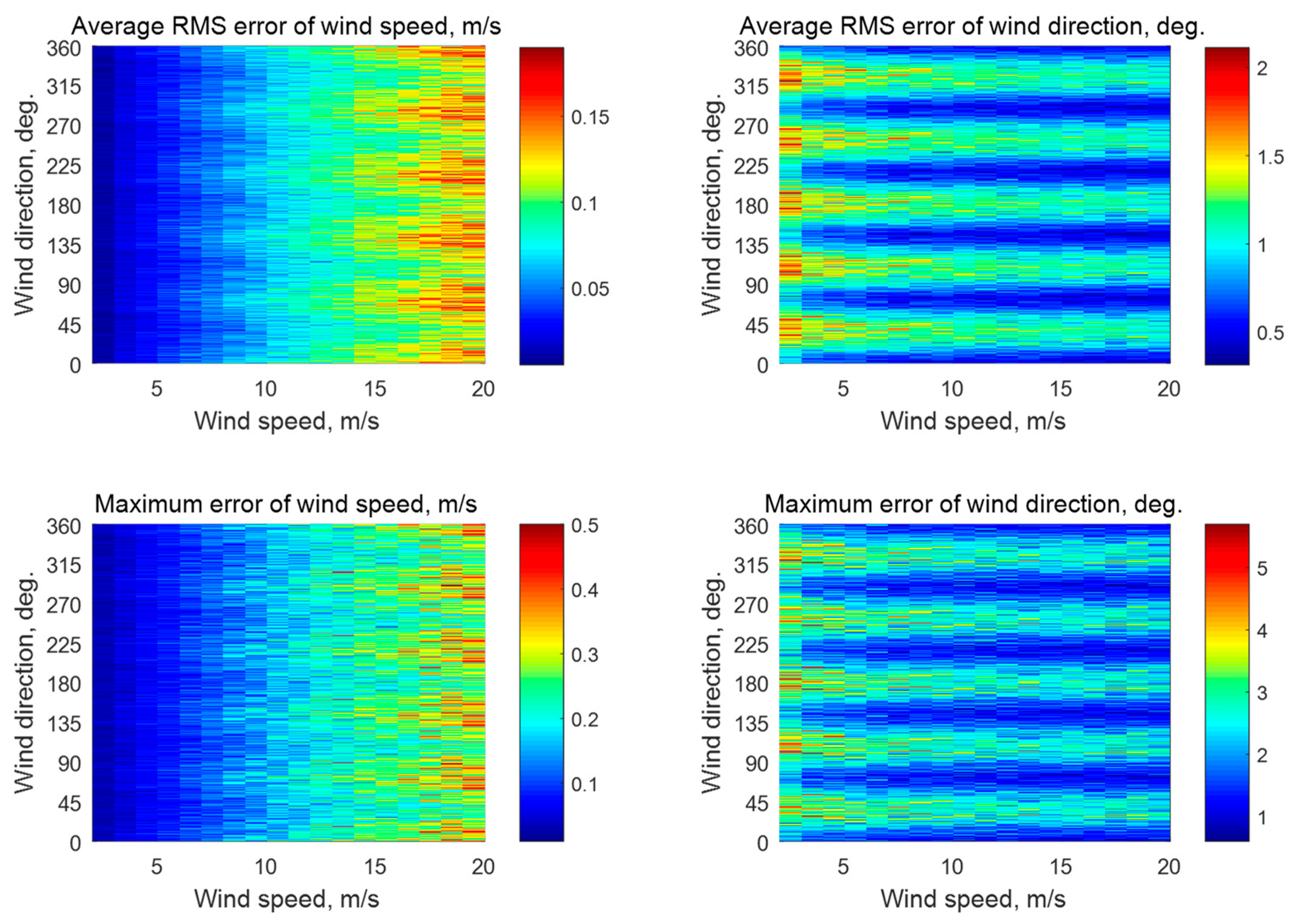
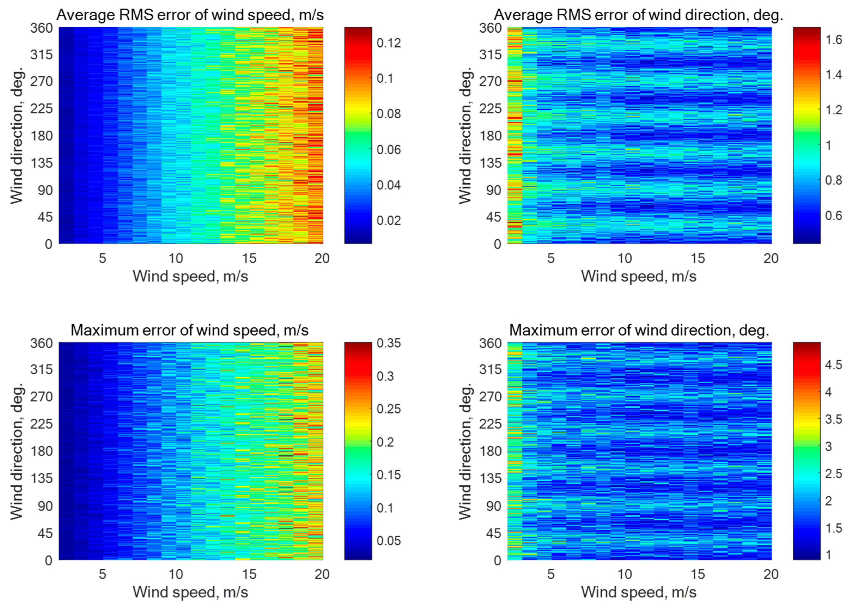
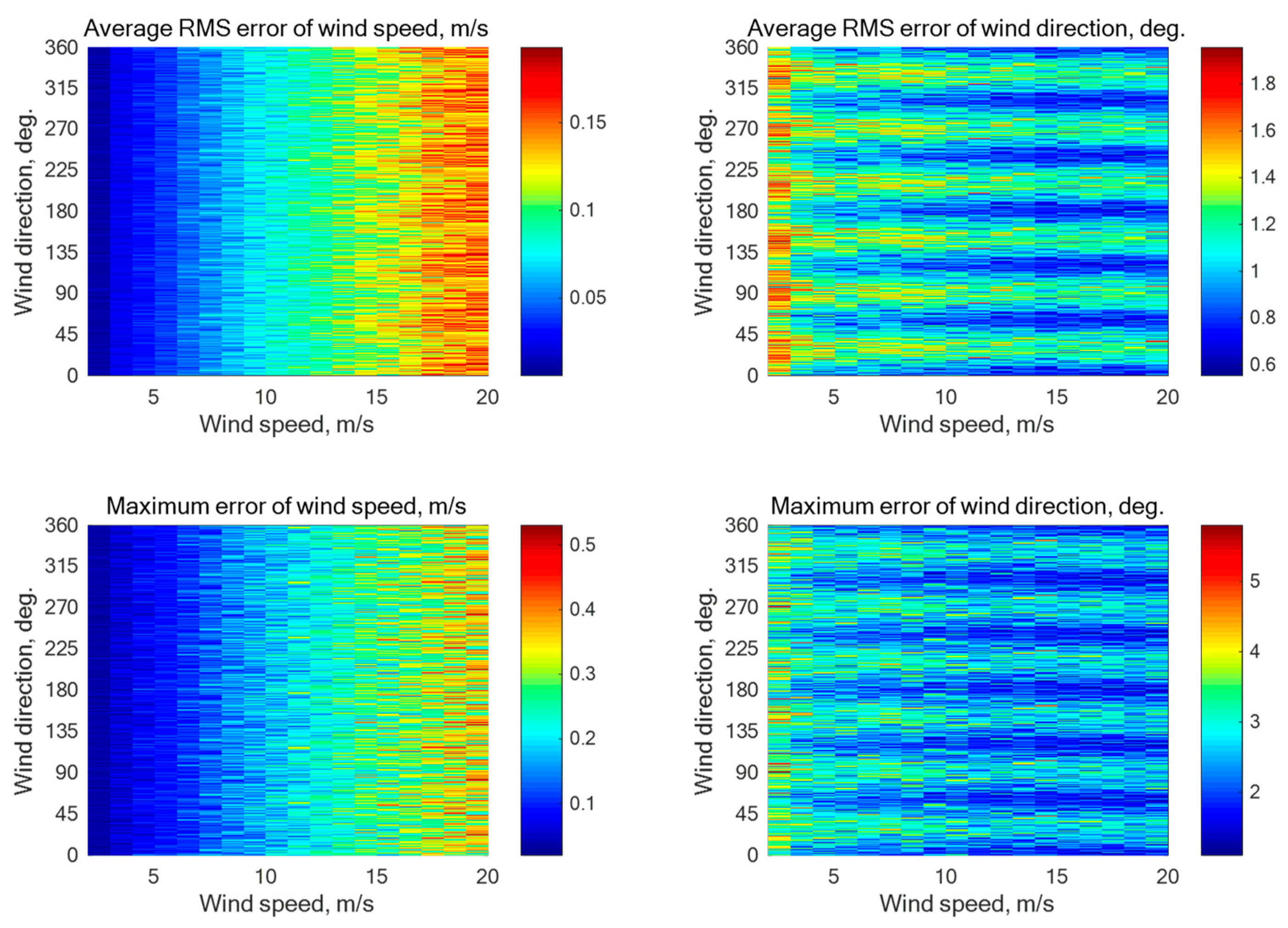
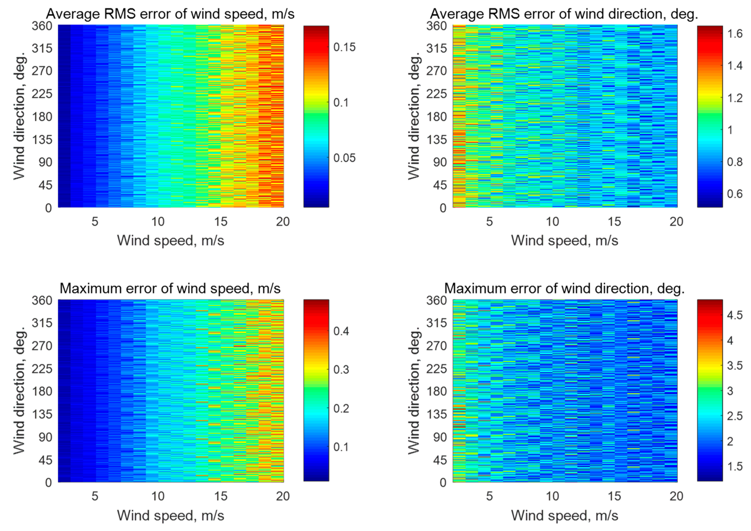
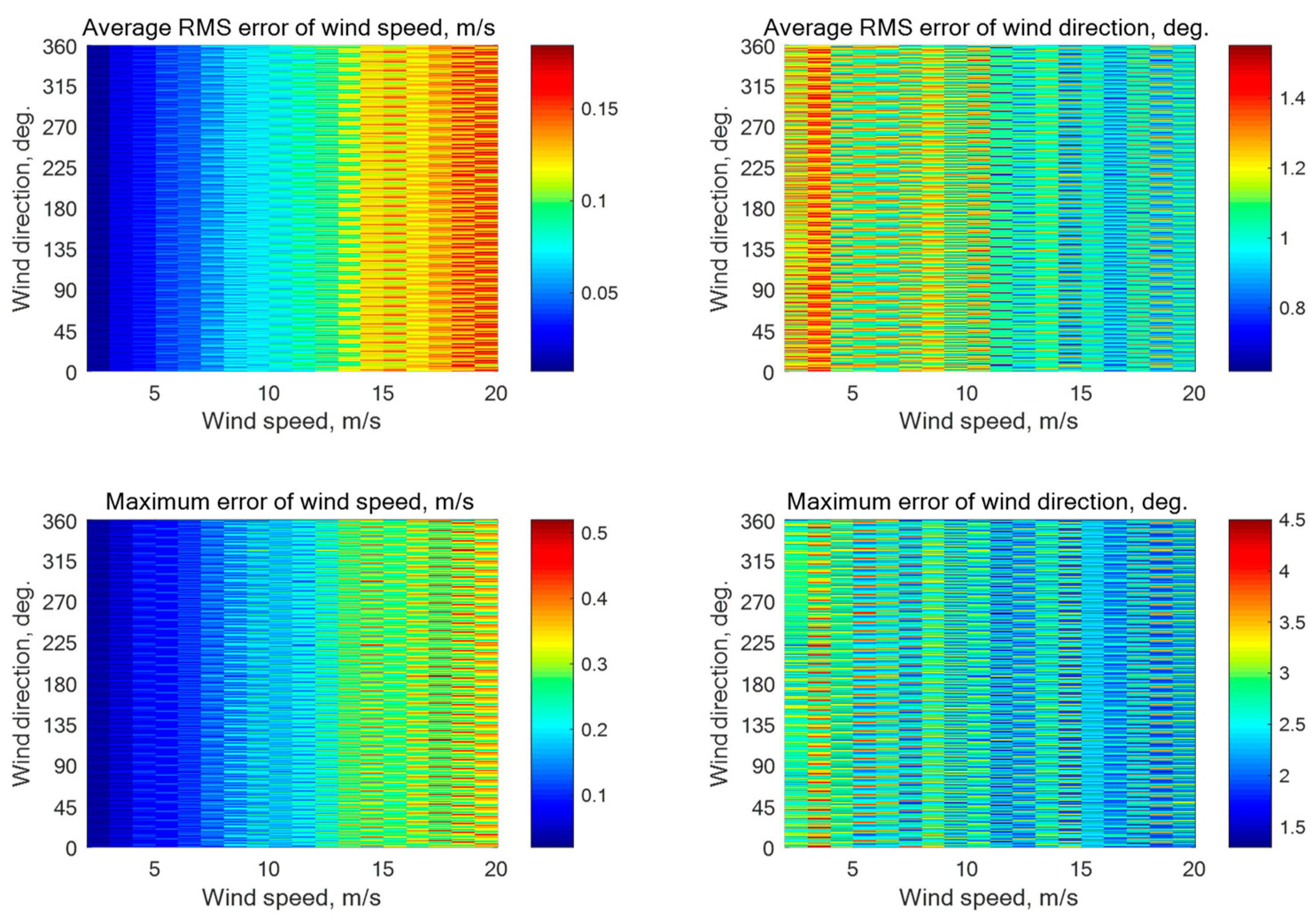
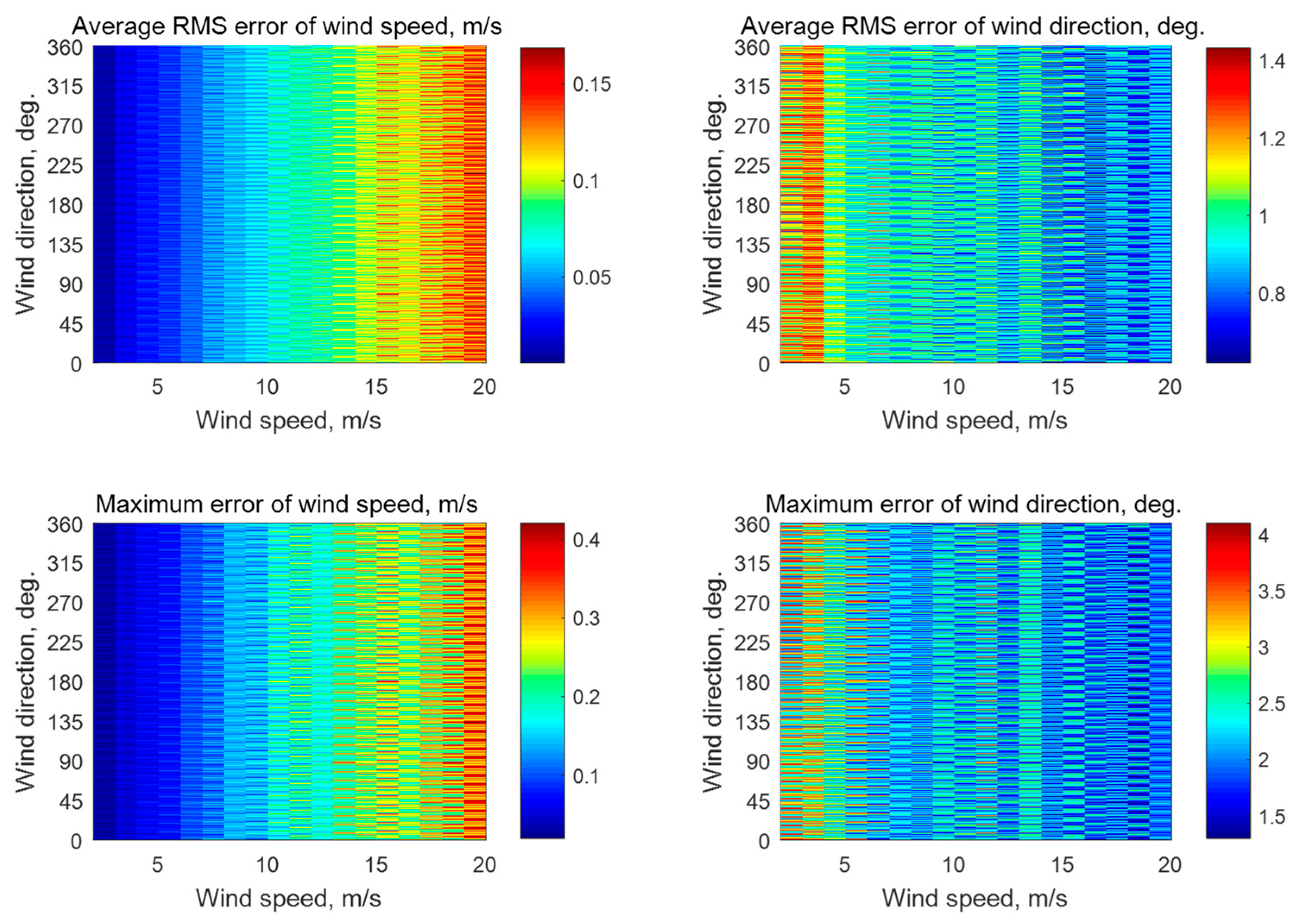
N = 5) is characterized by the beam directions of 0°, 72°, 144°, 216°, and 288° relative to the aircraft course. The number of ‘‘measured’’ NRCS samples averaged for each beam here is 4000 at the incidence angle of 30° and 1252 at the incidence angles of 45° or 60°. Simulations without additive instrumental noise have demonstrated the maximum errors of the wind speed and direction retrieval of 0.35 m/s and 3.7°, 0.64 m/s and 5.0°, and 0.5 m/s and 5.4°, respectively, at the incidence angles of 30°, 45°, and 60°. Simulation results with the instrumental noise assumption of 0.1 dB and 0.2 dB are summarized in
Figure A1,
Figure A2 and
Figure A3. The maximum errors are 0.36 m/s and 6.0°, 0.65 m/s and 6.1°, and 0.51 m/s and 5.7°, respectively, at the incidence angles of 30°, 45°, and 60°.
For the six-beam star geometry (
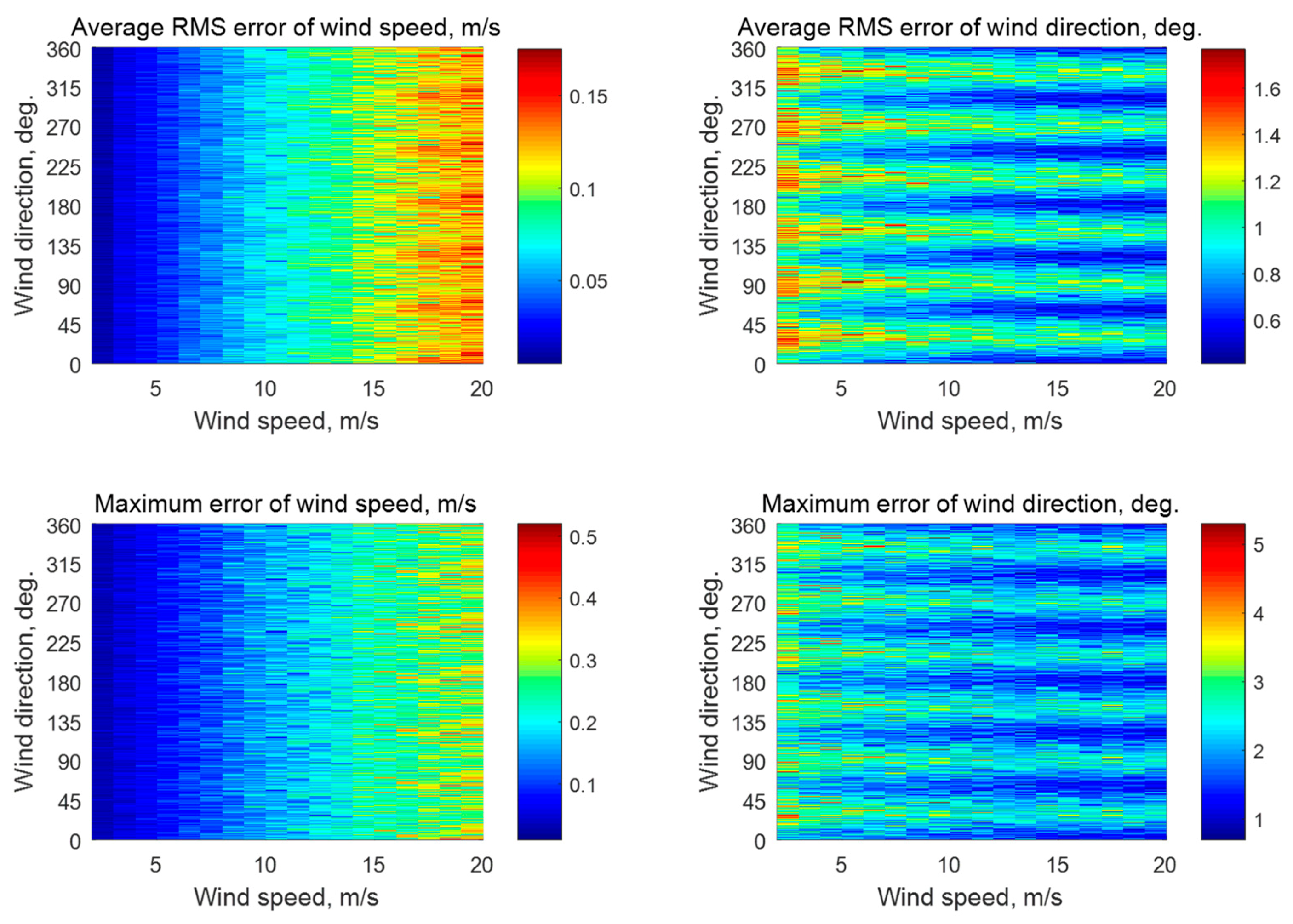
N = 6) with the beam directions of 0°, 60°, 120°, 180°, 240°, and 300° relative to the aircraft course, the number of ‘’measured’’ NRCS samples averaged for each beam is 3333 at the incidence angle of 30° and 1044 at the incidence angles of 45° or 60°. Simulations without instrumental noise have shown the maximum errors of the wind speed and direction retrieval of 0.35 m/s and 3.5°, 0.52 m/s and 4.6°, and 0.51 m/s and 5.1°, respectively, at the incidence angles of 30°, 45°, and 60°. Simulation results with the instrumental noise assumption of 0.1 dB and 0.2 dB are summarized in
Figure A4,
Figure A5 and
Figure A6. The maximum errors are 0.36 m/s and 4.9°, 0.53 m/s and 5.8°, and 0.52 m/s and 5.3° at the incidence angles of 30°, 45°, and 60°, respectively.
The eight-beam star geometry (
N = 8) has the beam directions of 0°, 45°, 90°, 135°, 180°, 225°, 270°, and 315° relative to the aircraft course. The number of ‘‘measured’’ NRCS samples averaged for each beam is 2500 at the incidence angle of 30° and 783 at the incidence angles of 45° or 60°. The simulations without instrumental noise have shown the maximum errors of the wind speed and direction retrieval of 0.33 m/s and 3.1°, 0.53 m/s and 5.0°, and 0.47 m/s and 4.2°, respectively, at the incidence angles of 30°, 45°, and 60°. The simulation results with the instrumental noise assumption of 0.1 dB and 0.2 dB are summarized in
Figure A7,
Figure A8 and
Figure A9, respectively. The maximum errors are 0.34 m/s and 4.9°, 0.54 m/s and 5.7°, and 0.48 m/s and 4.5°, respectively, at the incidence angles of 30°, 45°, and 60°.
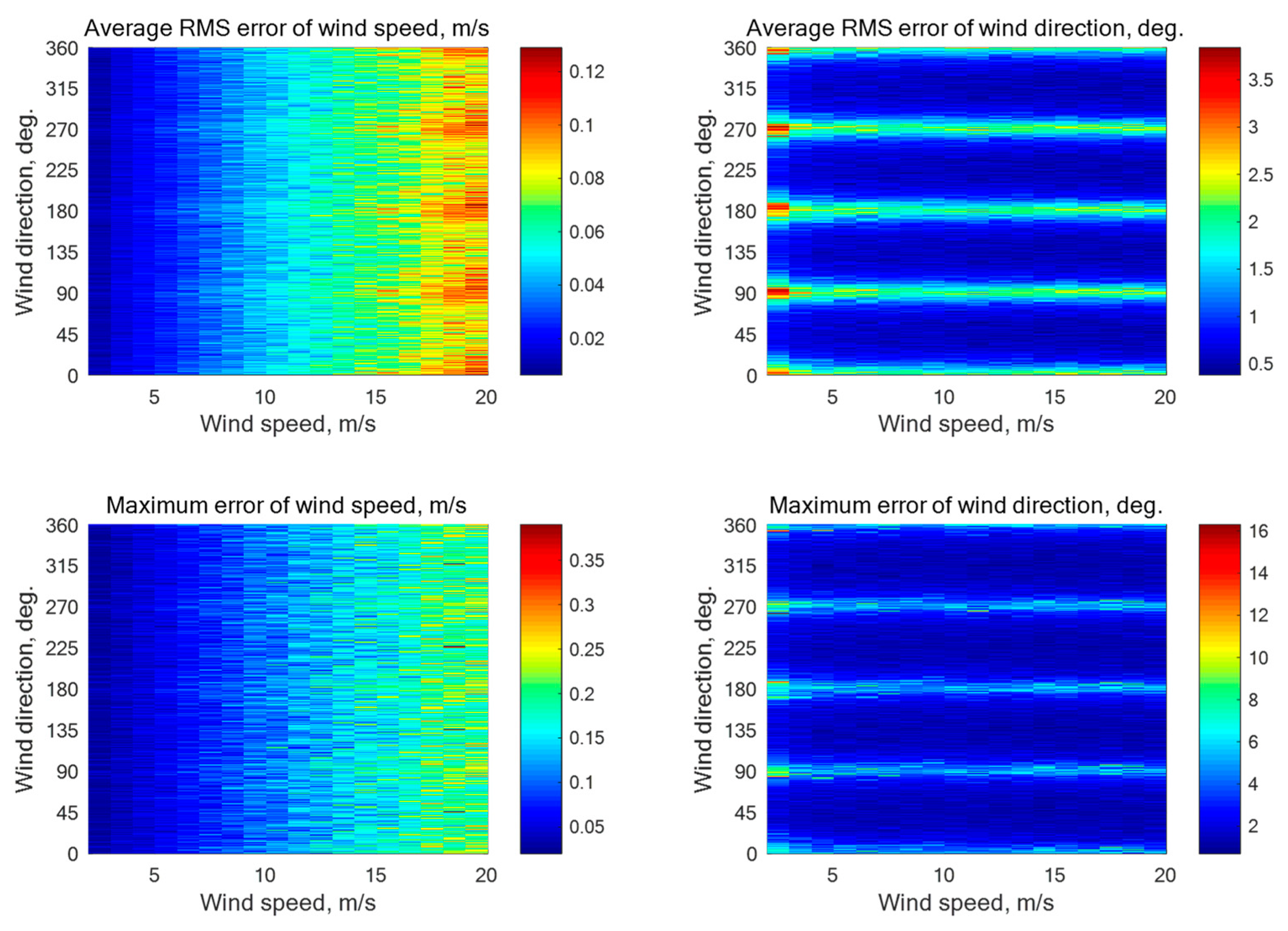
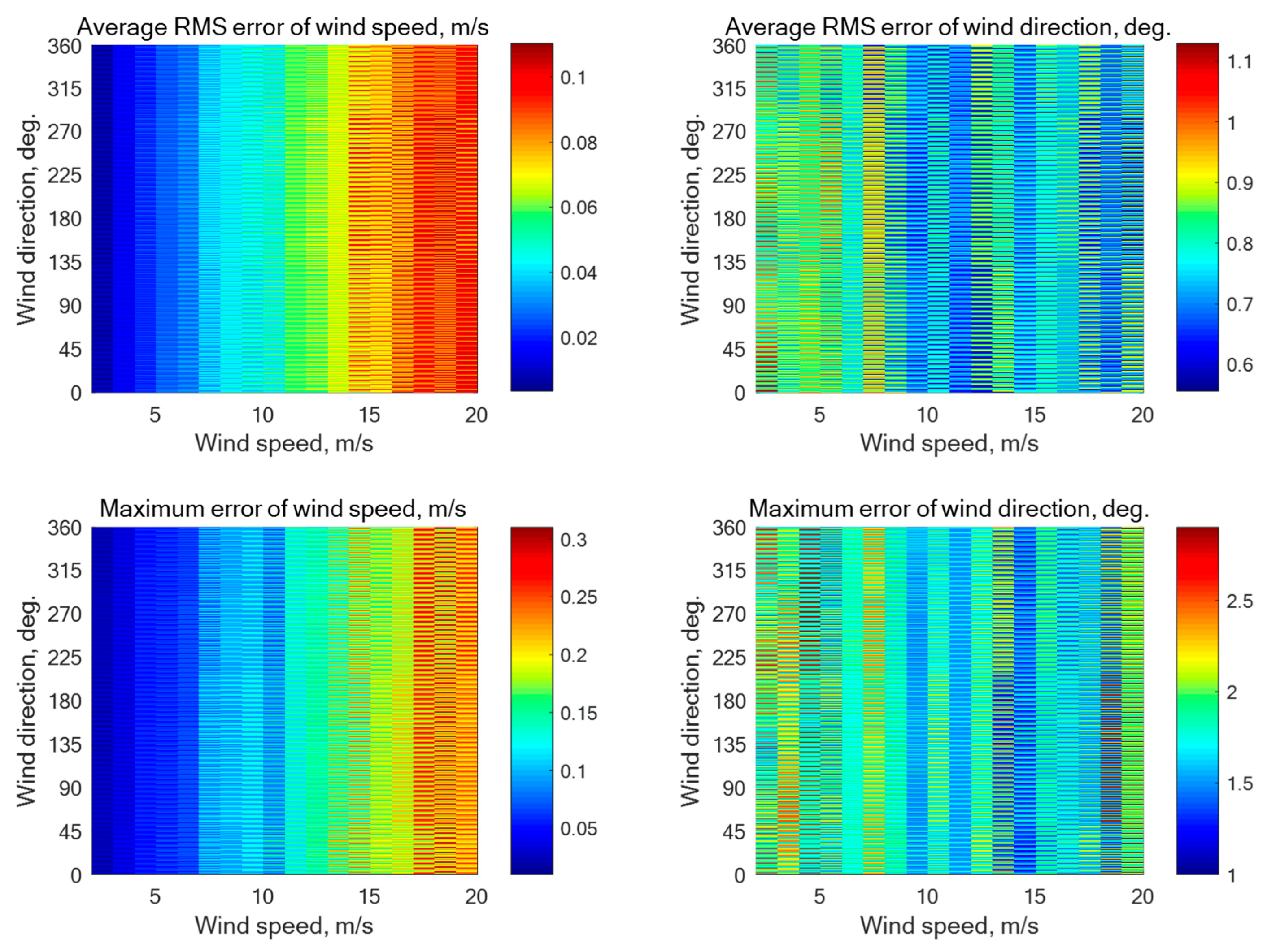
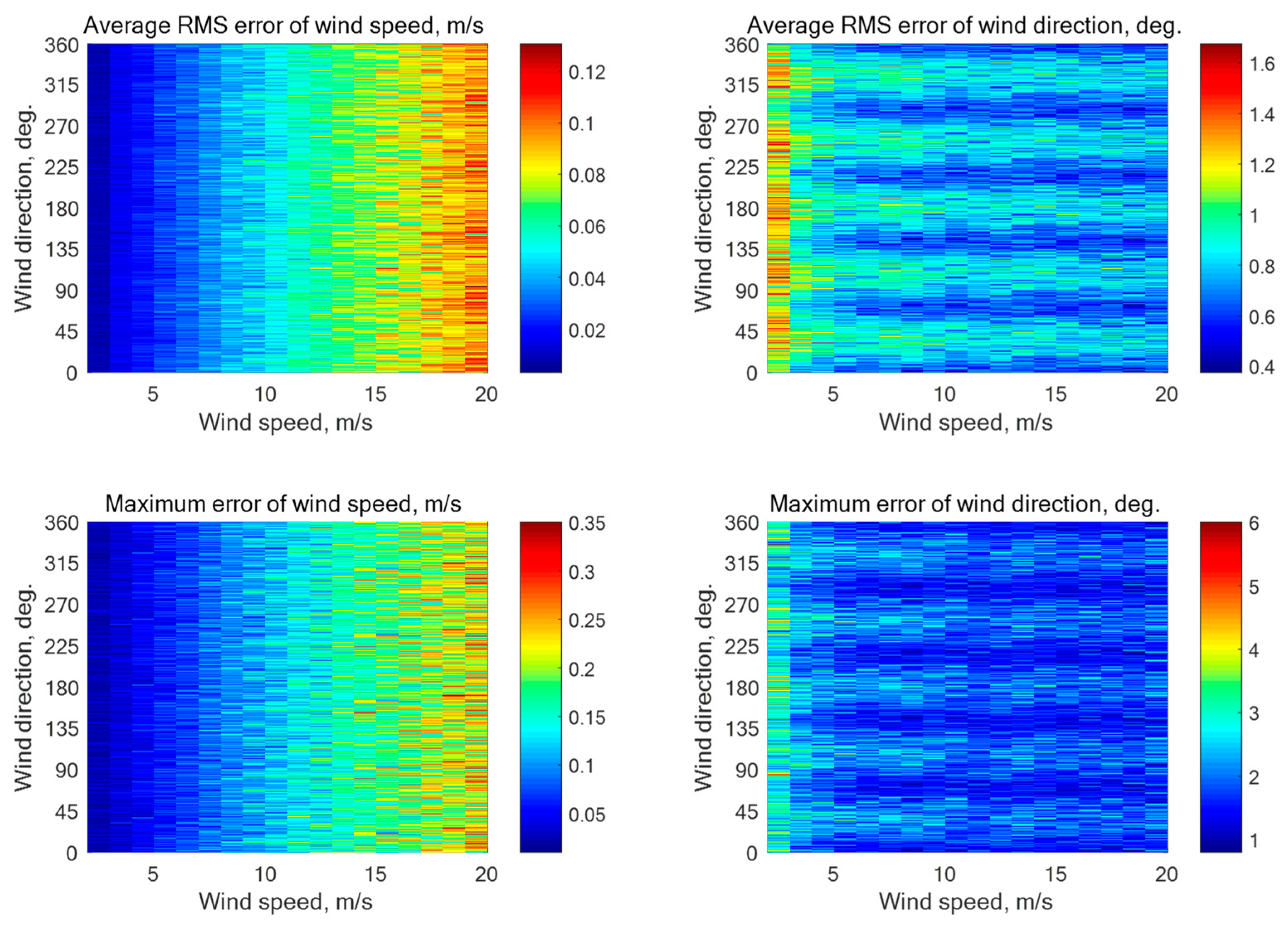
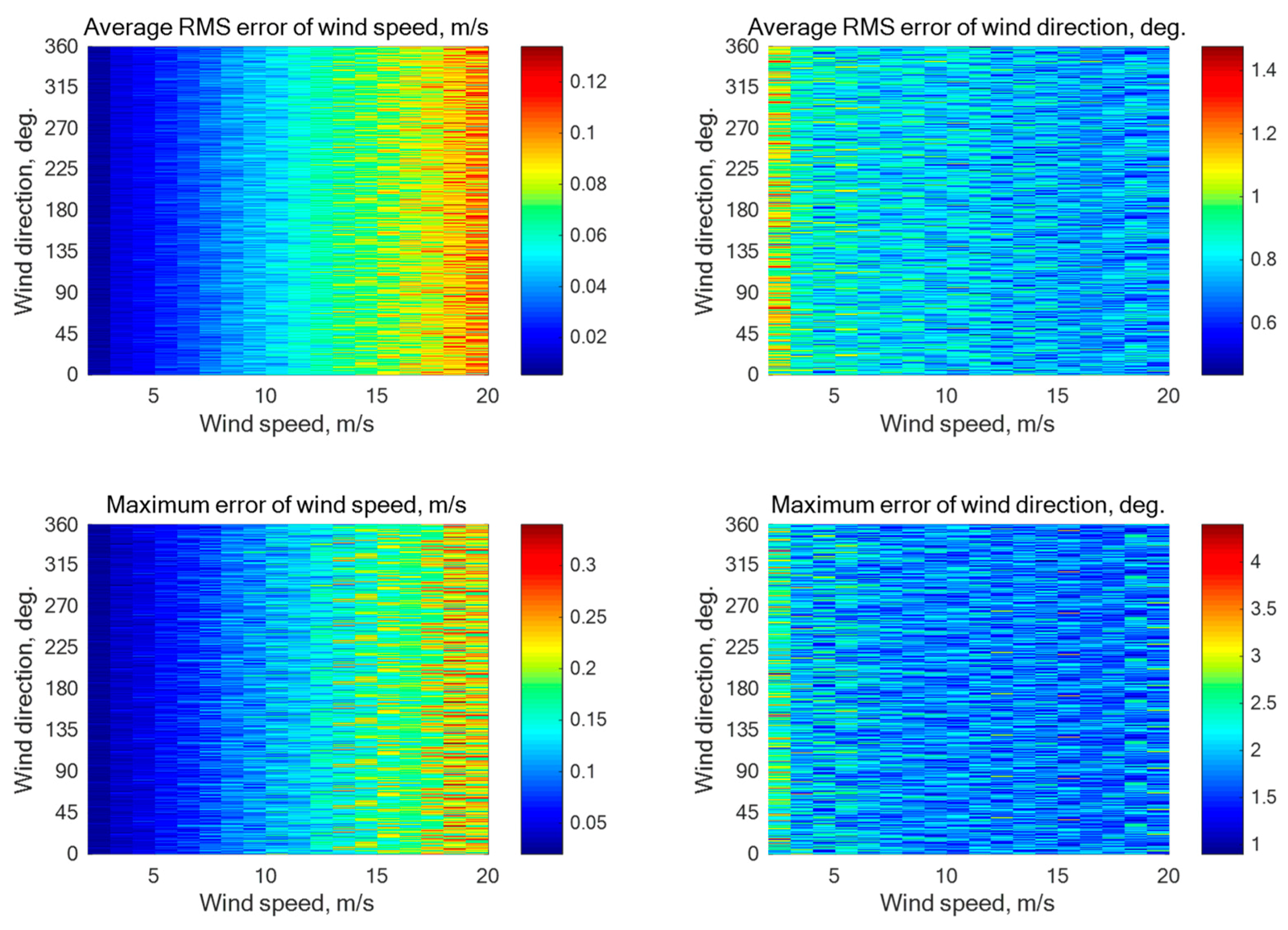
Figure A1.
Simulation results for a five-beam star geometry (N = 5) with the beam directions of 0°, 72°, 144°, 216°, and 288° relative to the aircraft course with an assumption of 0.1 dB instrumental noise at the wind speeds of 2–20 m/s for the incidence angle of 30° with 4000 averaged NRCS samples for each azimuthal angle.
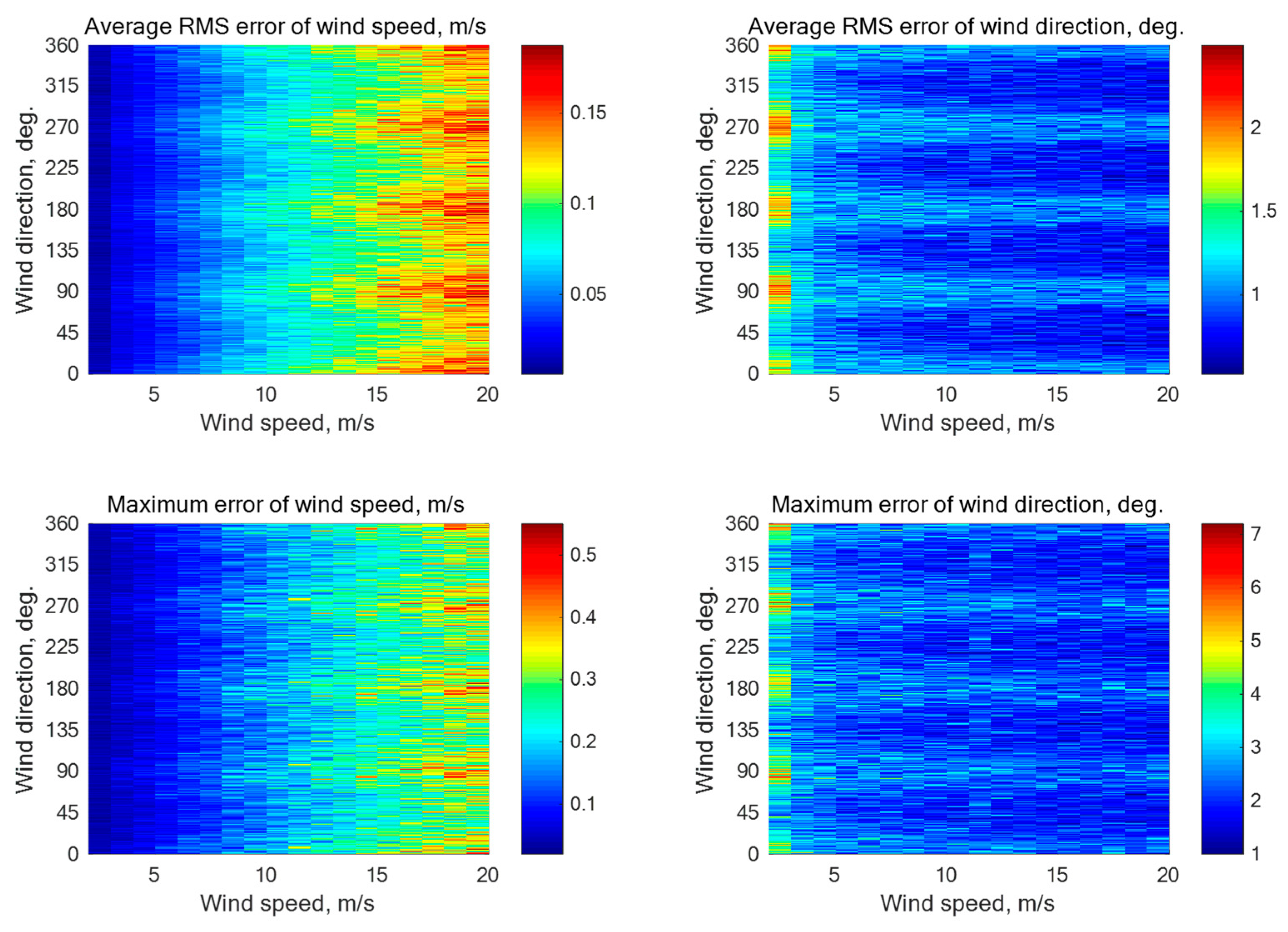
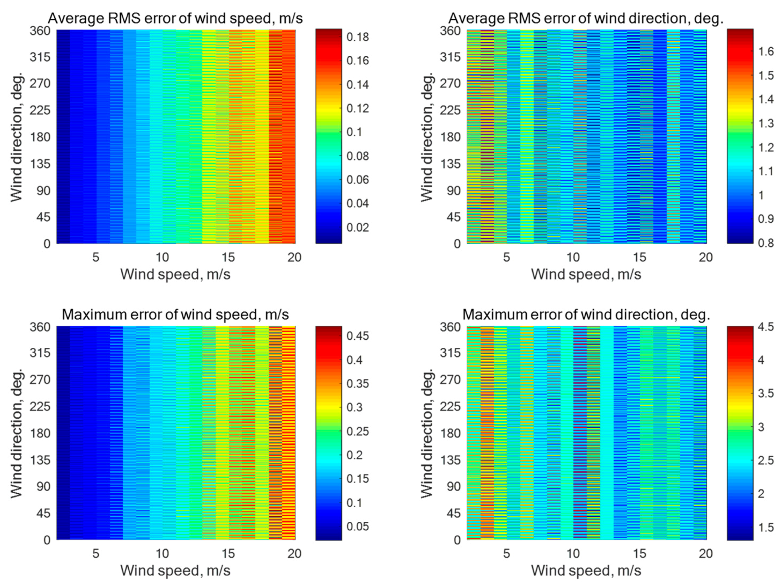
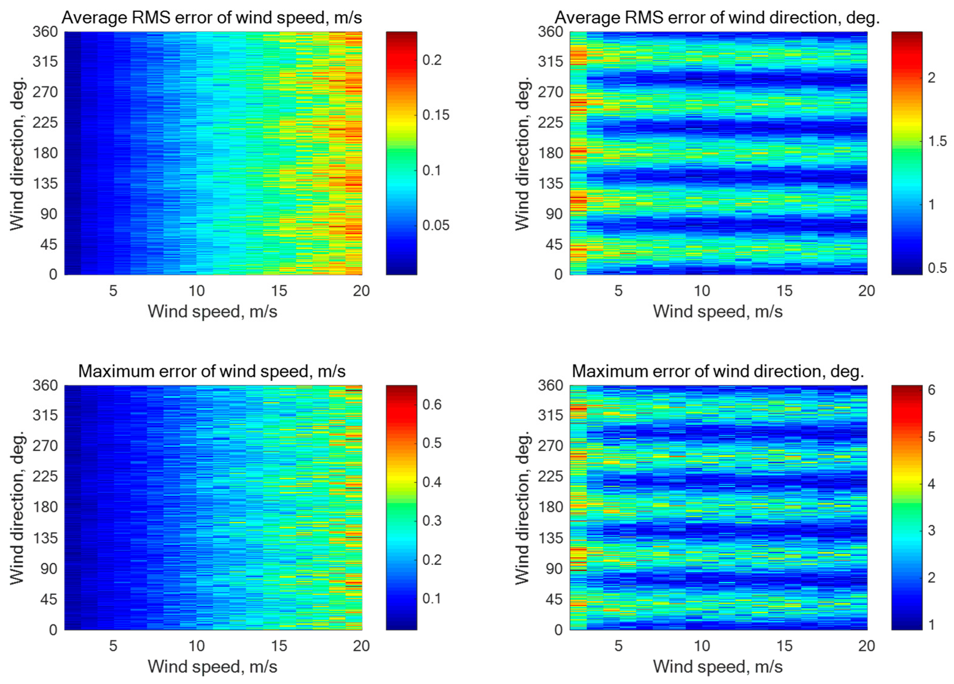
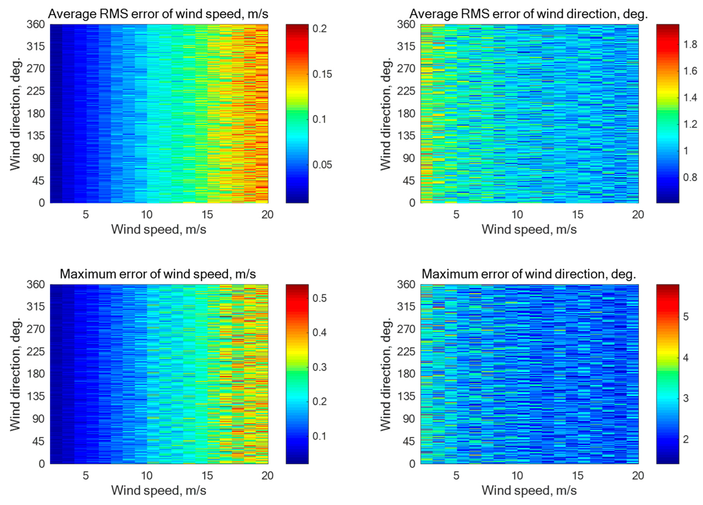
Figure A2.
Simulation results for a five-beam star geometry (N = 5) with the beam directions of 0°, 72°, 144°, 216°, and 288° relative to the aircraft course with an assumption of 0.2 dB instrumental noise at the wind speeds of 2–20 m/s for the incidence angle of 45° with 1252 averaged NRCS samples for each azimuthal angle.
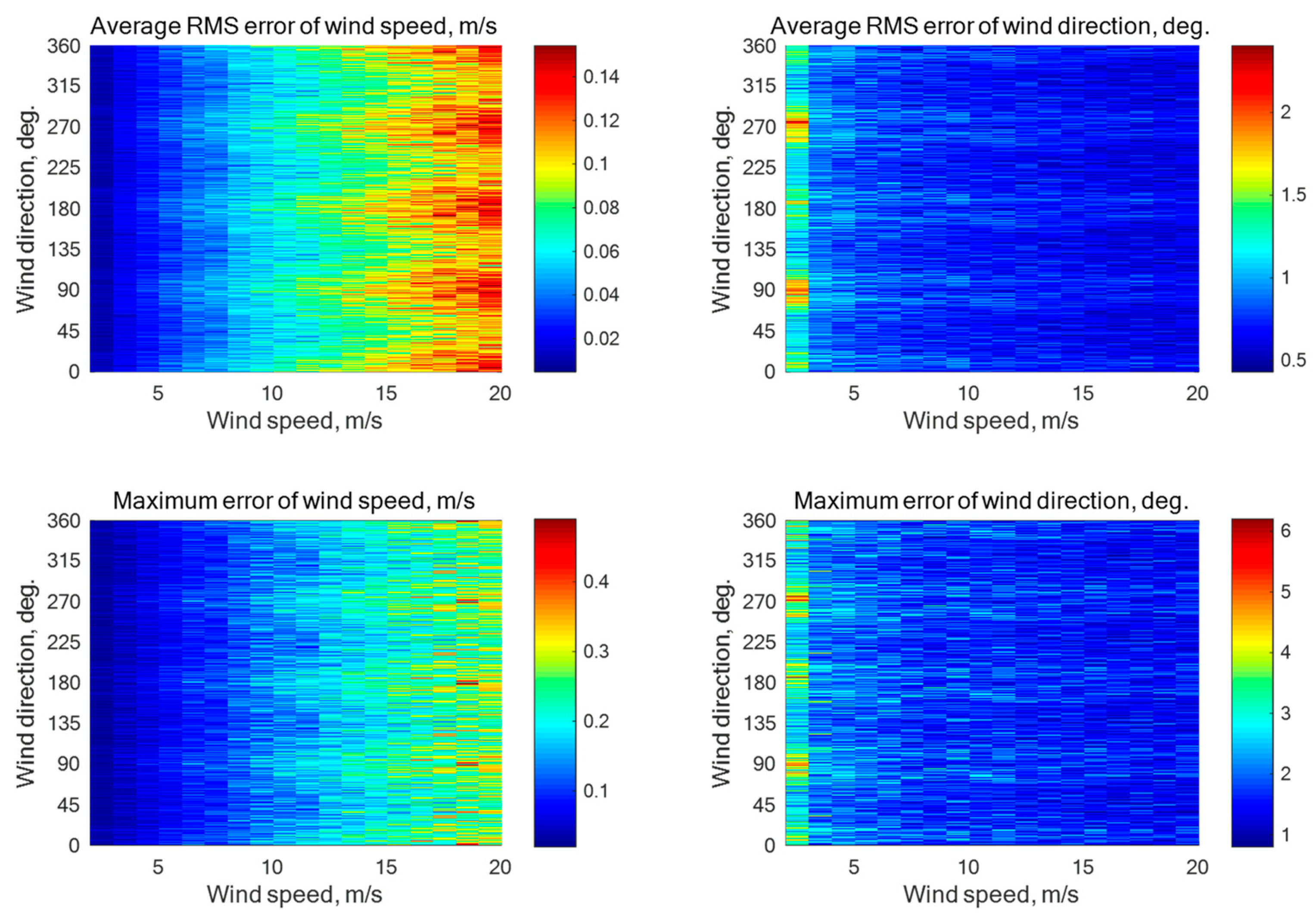
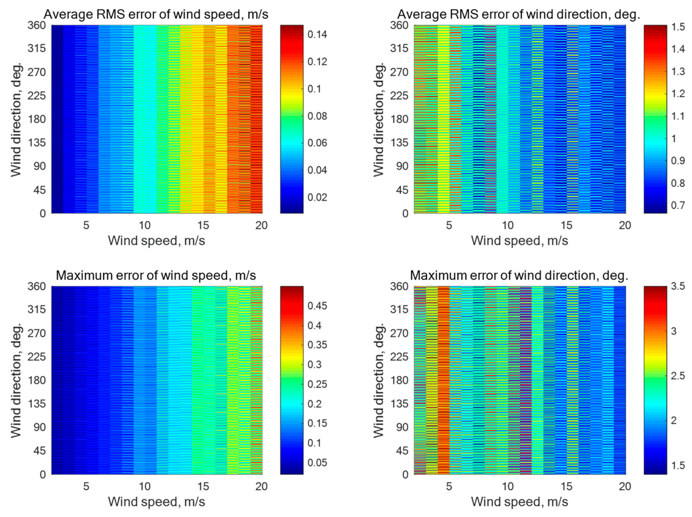
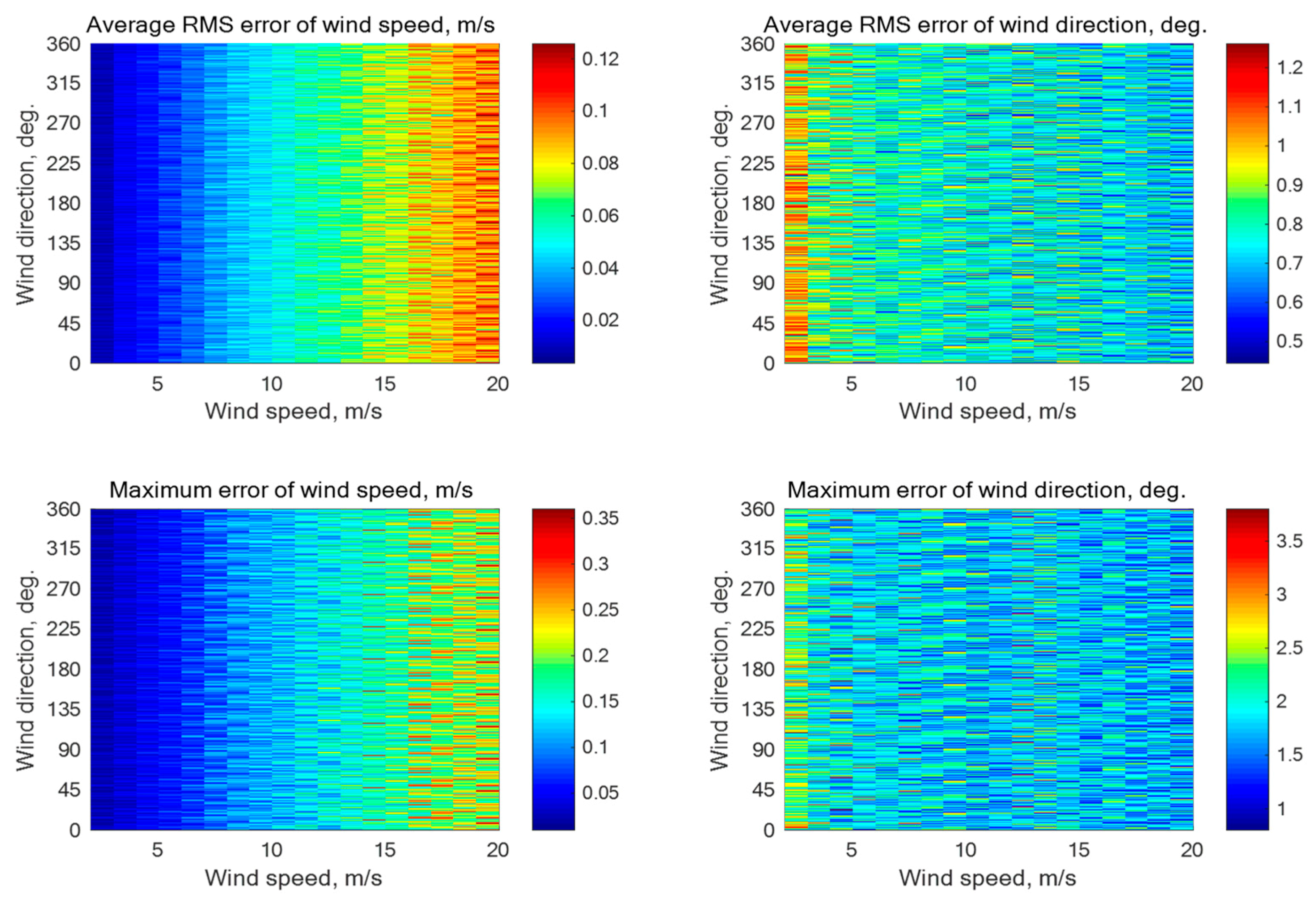
Figure A3.
Simulation results for a five-beam star geometry (N = 5) with the beam directions of 0°, 72°, 144°, 216°, and 288° relative to the aircraft course with an assumption of 0.2 dB instrumental noise at the wind speeds of 2–20 m/s for the incidence angle of 60° with 1252 averaged NRCS samples for each azimuthal angle.
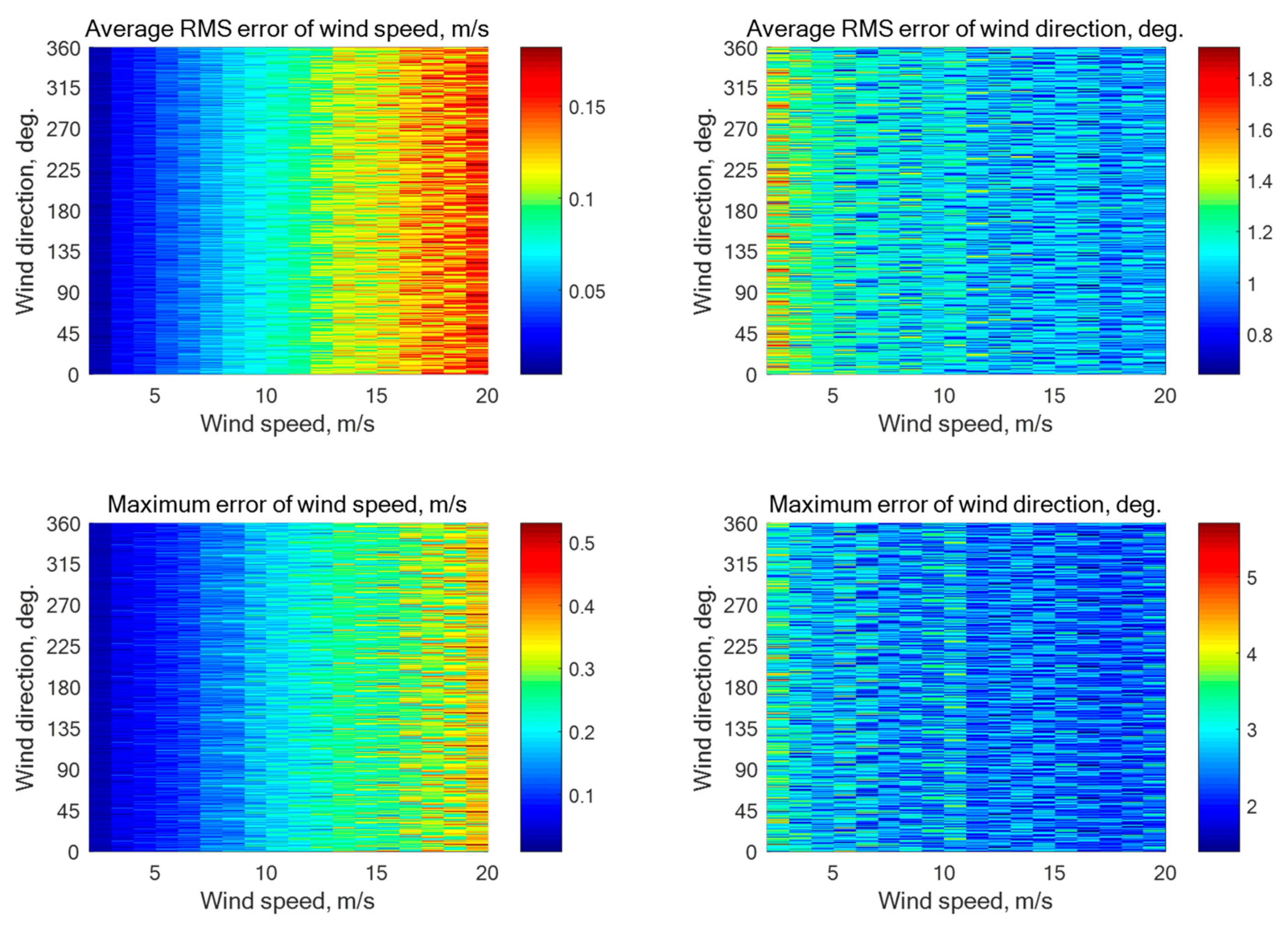
Figure A4.
Simulation results for a six-beam star geometry (N = 6) with the beam directions of 0°, 60°, 120°, 180°, 240°, and 300° relative to the aircraft course with an assumption of 0.1 dB instrumental noise at the wind speeds of 2–20 m/s for the incidence angle of 30° with 3333 averaged NRCS samples for each azimuthal angle.
Figure A5.
Simulation results for a six-beam star geometry (N = 6) with the beam directions of 0°, 60°, 120°, 180°, 240°, and 300° relative to the aircraft course with an assumption of 0.2 dB instrumental noise at the wind speeds of 2–20 m/s for the incidence angle of 45° with 1044 averaged NRCS samples for each azimuthal angle.
Figure A6.
Simulation results for a six-beam star geometry (N = 6) with the beam directions of 0°, 60°, 120°, 180°, 240°, and 300° relative to the aircraft course with an assumption of 0.2 dB instrumental noise at the wind speeds of 2–20 m/s for the incidence angle of 60° with 1044 averaged NRCS samples for each azimuthal angle.
Figure A7.
Simulation results for an eight-beam star geometry (N = 8) with the beam directions of 0°, 60°, 120°, 180°, 240°, and 300° relative to the aircraft course with an assumption of 0.1 dB instrumental noise at the wind speeds of 2–20 m/s for the incidence angle of 30° with 2500 averaged NRCS samples for each azimuthal angle.
Figure A8.
Simulation results for an eight-beam star geometry (N = 8) with the beam directions of 0°, 60°, 120°, 180°, 240°, and 300° relative to the aircraft course with an assumption of 0.2 dB instrumental noise at the wind speeds of 2–20 m/s for the incidence angle of 45° with 783 averaged NRCS samples for each azimuthal angle.
Figure A9.
Simulation results for an eight-beam star geometry (N = 8) with the beam directions of 0°, 60°, 120°, 180°, 240°, and 300° relative to the aircraft course with an assumption of 0.2 dB instrumental noise at the wind speeds of 2–20 m/s for the incidence angle of 60° with 783 averaged NRCS samples for each azimuthal angle.
For the ten-beam star geometry (
N = 10) with the beam directions of 0°, 36°, 72°, 108°, 144°, 180°, 216°, 252°, 288°, and 324° relative to the aircraft course, the number of ‘‘measured’’ NRCS samples averaged for each beam is 2000 at the incidence angle of 30° and 626 at the incidence angles of 45° or 60°. The simulations have shown that without instrumental noise the maximum errors of the wind speed and direction retrieval are 0.35 m/s and 3.5°, 0.53 m/s and 4.6°, and 0.48 m/s and 3.9°, respectively, at the incidence angles of 30°, 45°, and 60°. The simulation results with the instrumental noise assumption of 0.1 dB and 0.2 dB are presented in
Figure A10,
Figure A11 and
Figure A12, respectively. The maximum errors are 0.36 m/s and 3.8°, 0.54 m/s and 5.7°, and 0.49 m/s and 4.8°, respectively, at the incidence angles of 30°, 45°, and 60°.
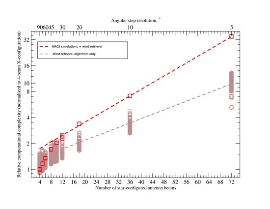
We have also performed simulations for twelve-beam geometry (
N = 12) and eighteen-beam geometry (
N=18). However, since in this range increasing
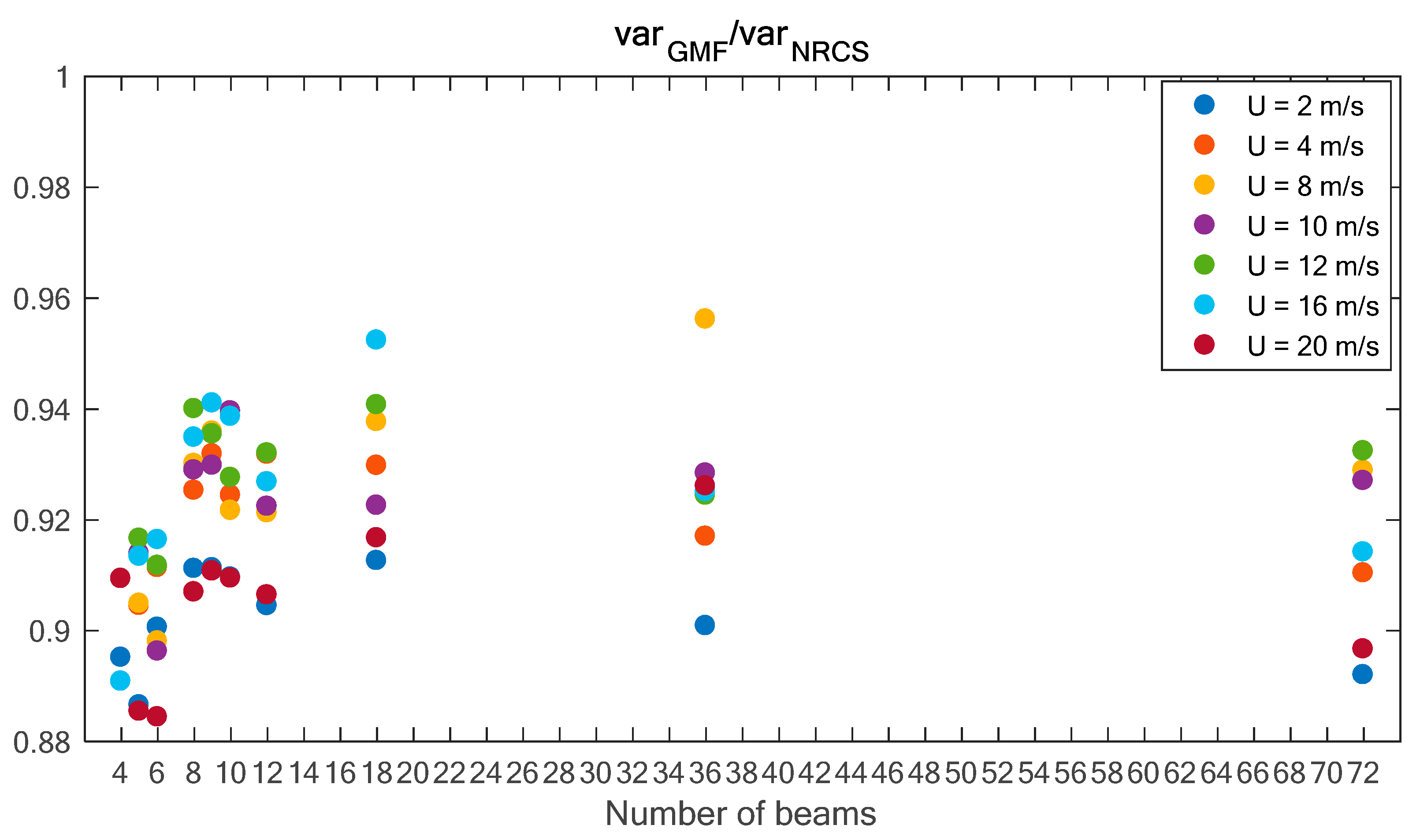
N leads to a very small adjustment in the angular resolution, and all results were qualitatively similar such that no additional conclusions could be drawn, to save space, we skip the corresponding figures. Of note, results for twelve- and eighteen-beam geometries are nevertheless used in the summary boxplots in the main text (see
Figure 7).
Next, a thirty-six-beam star geometry (
N = 36) characterized by the equiangular beams with a 10° increment angle, i.e., 0°, 10°, 20°, ..., 350° relative to the aircraft course are considered. The number of “measured” NRCS samples averaged for each beam is 556 at the incidence angle of 30° and 174 at the incidence angles of 45° or 60°. The simulations without instrumental noise have demonstrated the maximum errors of the wind speed and direction retrieval of 0.28 m/s and 3.0°, 0.51 m/s and 4.3°, and 0.41 m/s and 3.8°, respectively, at the incidence angles of 30°, 45°, and 60°. The simulation results with the instrumental noise assumption of 0.1 dB and 0.2 dB are presented in
Figure A13,
Figure A14 and
Figure A15, respectively. The maximum errors are 0.29 m/s and 3.1°, 0.52 m/s and 4.5°, and 0.42 m/s and 4.1°, respectively, at the incidence angles of 30°, 45°, and 60°.
Figure A10.
Simulation results for an eight-beam star geometry (N = 10) with the beam directions of 0°, 36°, 72°, 108°, 144°, 180°, 216°, 252°, 288°, and 324° relative to the aircraft course with an assumption of 0.1 dB instrumental noise at the wind speeds of 2–20 m/s for the incidence angle of 30° with 2000 averaged NRCS samples for each azimuthal angle.
Figure A11.
Simulation results for a ten-beam star geometry (N = 10) with the beam directions of 0°, 36°, 72°, 108°, 144°, 180°, 216°, 252°, 288°, and 324° relative to the aircraft course with an assumption of 0.2 dB instrumental noise at the wind speeds of 2–20 m/s for the incidence angle of 45° with 626 averaged NRCS samples for each azimuthal angle.
Figure A12.
Simulation results for a ten-beam star geometry (N = 10) with the beam directions of 0°, 36°, 72°, 108°, 144°, 180°, 216°, 252°, 288°, and 324° relative to the aircraft course with an assumption of 0.2 dB instrumental noise at the wind speeds of 2–20 m/s for the incidence angle of 60° with 626 averaged NRCS samples for each azimuthal angle.
Figure A13.
Simulation results for a thirty-six-beam star geometry (N = 36) with the beam directions of 0°, 10°, 20°, 30°, 40°, 50°, 60°, 70°, 80°, 90°, 100°, 110°, 120°, 130°, 140°, 150°, 160°, 170°, 180°, 190°, 200°, 210°, 220°, 230°, 240°, 250°, 260°, 270°, 280°, 290°, 300°, 310°, 320°, 330°, 340°, and 350° relative to the aircraft course with an assumption of 0.1 dB instrumental noise at the wind speeds of 2–20 m/s for the incidence angle of 30° with 556 averaged NRCS samples for each azimuthal angle.
Figure A14.
Simulation results for a thirty-six-beam star geometry (N = 36) with the beam directions of 0°, 10°, 20°, 30°, 40°, 50°, 60°, 70°, 80°, 90°, 100°, 110°, 120°, 130°, 140°, 150°, 160°, 170°, 180°, 190°, 200°, 210°, 220°, 230°, 240°, 250°, 260°, 270°, 280°, 290°, 300°, 310°, 320°, 330°, 340°, and 350° relative to the aircraft course with an assumption of 0.2 dB instrumental noise at the wind speeds of 2–20 m/s for the incidence angle of 45° with 174 averaged NRCS samples for each azimuthal angle.
Figure A15.
Simulation results for a thirty-six-beam star geometry (N = 36) with the beam directions of 0°, 10°, 20°, 30°, 40°, 50°, 60°, 70°, 80°, 90°, 100°, 110°, 120°, 130°, 140°, 150°, 160°, 170°, 180°, 190°, 200°, 210°, 220°, 230°, 240°, 250°, 260°, 270°, 280°, 290°, 300°, 310°, 320°, 330°, 340°, and 350° relative to the aircraft course with an assumption of 0.2 dB instrumental noise at the wind speeds of 2–20 m/s for the incidence angle of 60° with 174 averaged NRCS samples for each azimuthal angle.

 ,
, 


