Development and Performance Assessment of a Low-Cost UAV Laser Scanner System (LasUAV)

Abstract

This study reports on a low-cost unmanned aerial vehicle (UAV)-borne light detection and ranging (LiDAR) system called LasUAV, from hardware selection and integration to the generation of three-dimensional point clouds, and an assessment of its performance. Measurement uncertainties were estimated in angular static, angular dynamic, and real flight conditions. The results of these experiments indicate that the point cloud elevation accuracy in the case of angular static acquisition was 3.8 cm, and increased to 3.9 cm in angular dynamic acquisition. In-flight data were acquired over a target surveyed by nine single passages in different flight directions and platform orientations. In this case, the uncertainty of elevation ranged between 5.1 cm and 9.8 cm for each single passage. The combined elevation uncertainty in the case of multiple passages (i.e., the combination of one to nine passages from the set of nine passages) ranged between 5 cm (one passage) and 16 cm (nine passages). The study demonstrates that the positioning device, i.e., the Global Navigation Satellite System real-time kinematic (GNSS RTK) receiver, is the sensor that mostly influences the system performance, followed by the attitude measurement device and the laser sensor. Consequently, strong efforts and greater economic investment should be devoted to GNSS RTK receivers in low-cost custom integrated systems.

1. Introduction

Laser scanning (LS), also referred to as light detection and ranging (LiDAR), is a well-established and consolidated technology used extensively for environmental sciences. LS for aerial platforms, known as airborne laser scanning (ALS), has been used since 1994, when commercial systems became available [1]. The elevation accuracy of state-of-the-art ALS systems is down to 10 cm [2,3], while planimetric accuracy ranges between 3 and 35 cm at a 1000 m flying height, depending on the accuracy of the laser scanner sensor and inertial navigation system (INS) [3].

Nowadays, ALS is mostly used for mapping and monitoring extensive areas for topographic, urban, and hydrogeological purposes. ALS also provides data for research and operational applications related to the management of forest ecosystems, although data for forestry applications are often not acquired by dedicated flights, but are generated as a byproduct of the above-mentioned campaigns (i.e., land planning and monitoring). Therefore, they are frequently characterized by a low point density and, above all, are usually acquired in winter to minimize the disturbance of vegetation [4], leading to a systematic, significant tree height underestimation [5]. Being expensive, ALS in forestry is only affordable for large-scale continuous forest cover (e.g., Canada, USA, Scandinavian countries) and is less convenient where the forest cover is fragmented, as in most European countries.

Unmanned aerial vehicles (UAVs) are new platforms that have been used increasingly over the last decade to collect data for forest research, thanks to the miniaturization and cost reduction of Global Navigation Satellite System (GNSS) receivers, INS, computers, and remote sensing sensors [6].

Extremely compact laser scanners based on larger aerial versions have been developed in the last 10 years. On the basis of these developments, it became possible to operate LiDAR sensors integrated into UAVs [7,8]. Manufacturers such as Velodyne LiDAR Inc. (San Jose, CA, USA), Routescene Inc. (Edinburgh, UK), LeddarTech Inc. (Quebec City, QC, Canada), RIEGL Laser Measurement System GmbH (Horn, Austria), and Geodetics Inc. (San Diego, CA, USA) have developed small and fully integrated LiDAR sensors for UAVs. In those cases, a number of independent elements are integrated into a single device that is able to emit a laser pulse, record the back-scattered signal, measure the distance, retrieve the plane position and attitude, and compute the echo position. However, the high cost (in the range of 60–80 k€) of such integrated LiDAR systems makes their regular use only possible for very large projects, and the cost per unit of mapped surface is still higher than airborne systems. For these reasons, the use of such systems in environmental monitoring and forestry is still greatly limited. Airborne laser scanning acquisitions still remain profitable in economic terms, but UAV-borne laser scanning acquisitions allow greater flexibility with respect to the time period of acquisition and surface to be surveyed. In fact, flight repetitions over the same area over time are easier with UAVs and make unmanned LS more adaptable than ALS to monitoring variables with a higher frequency.

In contrast to the aerial platforms, the automotive markets have recently developed laser scanner devices, used for scene mapping, obstacle detection and avoidance, and autonomous driving, that have a lower cost due to the larger dimensions of the underlying market with respect to the aerial one, e.g., ibeo Automotive Systems GmbH (Hamburg, Germany), Lasea Inc. (Liège, Belgium), and Valeo Inc. (Paris, France). To be used in a laser scanner system, such laser sensors have to be integrated with other sensors, and procedures for data acquisition, synchronization, and processing have to be developed, which is quite challenging. There are few worldwide cases of LiDAR system development in research institutes. Choi et al. [9] developed a light and flexible UAV-based system at a low cost to perform rapid mapping for an emergency response. Nagai et al. [10] developed a system based on the combination of charge-coupled device (CCD) cameras, a laser scanner, an INS, and GNSS for a UAV-borne three-dimensional (3D) mapping system, which has been experimentally used in recovery efforts after natural disasters (e.g., landslides, river flooding). Jaakkola et al. [11] developed a low-cost mini-UAV-based laser scanning system, also capable of performing car-based mobile mapping, for tree measurements. Lin et al. [12] developed a mini-UAV-borne LiDAR system and the associated data processing involved in the coordinate triple, pulse intensity, and multi-echoes per pulse extraction for fine-scale mapping (e.g., tree height estimation, pole detection, road extraction, and digital terrain model refinement). Wallace et al. [13] developed a low-cost UAV-LiDAR system and the accompanying workflow to produce 3D point clouds with application in the forest inventory. Takahashi et al. [14] developed a small UAV-based laser scanner system for rice monitoring at low altitudes, while Christiansen [15] designed and tested a UAV mapping system for agricultural field surveying. Chiang et al. [16] developed a LiDAR-based UAV for surveys in impacted areas to collect geospatial data useful in disaster management and environment reconstruction planning.

In general, the overall budget for developing a UAV laser scanner system is quite challenging and the time required to develop the system [9,10,11,12,13,14,15,16] is more than two years. For instance, Choi et al. [9] had about 6 million USD at their disposal to spend in four years. In projects without such a large budget available, efforts in system development should be put toward containing the costs of subcomponents [11,12,15,16].

In addition, as there is no reliable, quick, cheap, and handy method for acquiring accurate high-resolution 3D data on objects in outdoor and moving environments with a laser scanner [10], in most cases, a laser scanner in combination with another sensor (CCD cameras and high-definition video cameras) is used [10,13]. Efforts in the development of LasUAV have been concentrated on developing a system that is much lower in cost than what is currently offered in the market and streamlining the procedures to produce the point cloud.

Costly integrated solutions are, in principle, more accurate, but the accuracy of an integrated LiDAR system comes from the combination of sources of uncertainty originating from the laser, positioning, and INS sensors. Thus, the optimal trade-off between cost and desired accuracy is hard to find when developing or purchasing a LiDAR system. If, for example, very accurate INS attitude data are coupled with relatively inaccurate laser sensors, or vice versa, the system will not be well balanced in terms of cost versus accuracy.

For the UAV laser scanner system (LasUAV) which was developed by a research project that lasted two years and is presented in this paper, a compromise between development time, cost, and linearity in the point cloud processing process was reached considering the limited resources available.

The aims of this paper are as follows: (i) to present in detail the development of a new low-cost laser scanner system capable of being used in environmental and forestry applications on an operational basis due to the low investment cost; (ii) to assess uncertainties associated with the different components of the system and their impact on total uncertainty; (iii) to quantify the optimum balance among system subcomponents; and (iv) to provide guidelines both for the development of a laser scanner system and for its optimal operation in specific applications.

We first describe the LiDAR system in terms of the integration of the sensors and the platform, and then present the data post processing and LiDAR point cloud generation. After that, we describe the performance assessment of the laser scanner system, and finally, we provide guidelines on the integration of LiDAR system components on the basis of the results obtained from our analysis.

2. Materials and Methods

2.1. The Sensors of LasUAV and UAV

The following sensors, with descriptions of their specific characteristics, were used to develop the LasUAV laser scanner system.

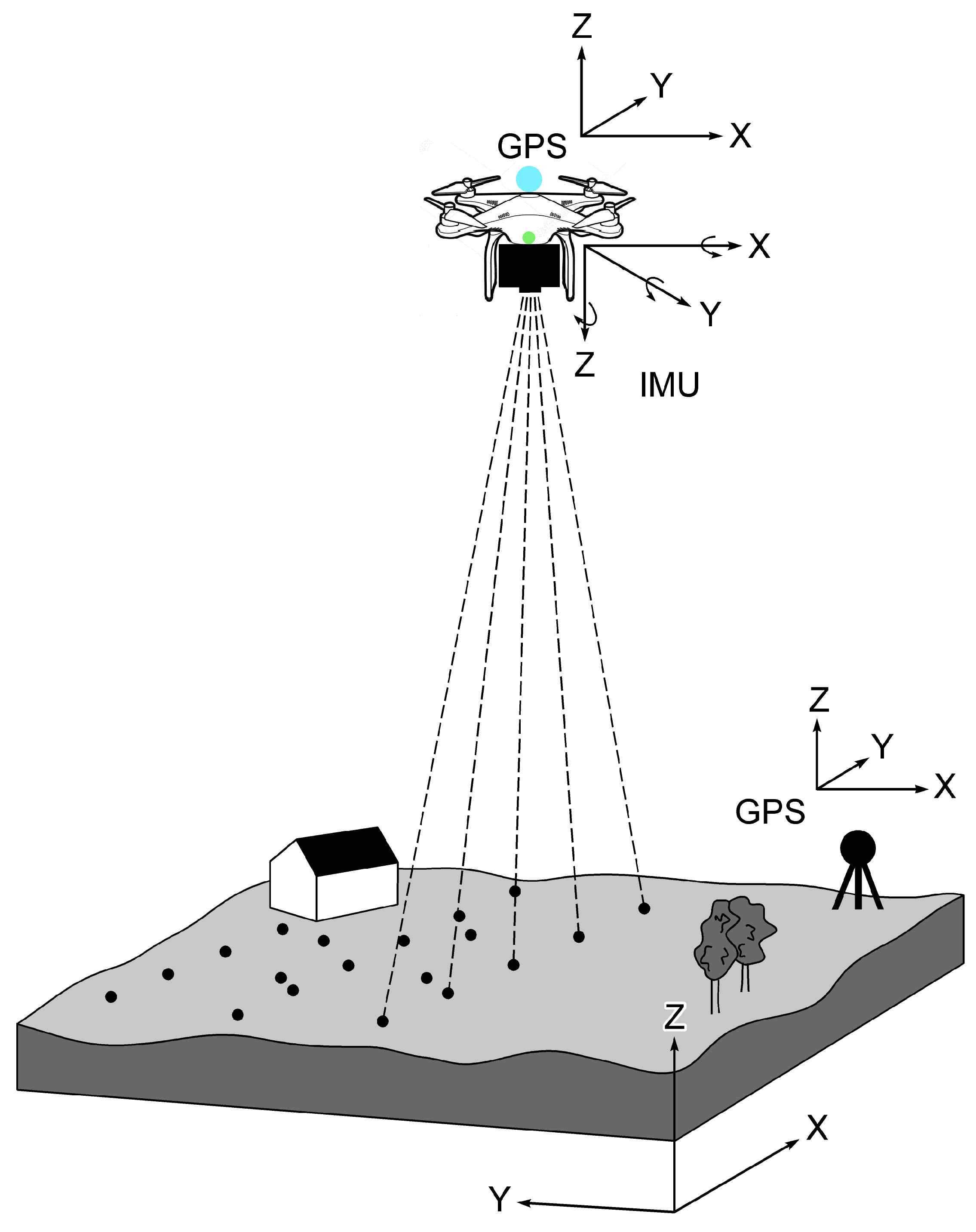
As an ALS system, the principle of measurement of UAV-borne laser scanning is based on laser-ranging measurements supported by position and orientation information derived with the use of a GNSS device and an INS (or an inertial measurement unit, IMU) mounted on a drone (Figure 1).

The laser scanner is the LUX 4L (ibeo Automotive Systems GmbH, Germany), a multilayer and multiecho laser scanner, i.e., it scans and measures in four parallel layers, each with a nominal transversal beam divergence of 0.8°, able to record up to three returns per pulse. The horizontal field of view (HFOV) is 110° (50° to −60°) in two layers and 85° (35° to −50°) in four layers. It can scan at a rate of 12.5, 25.0, or 50.0 Hz. The ibeo LUX 4L is able to detect targets at a maximum range of 200 m. The laser scanner was set to scan at a frequency of 12.5 Hz, the HFOV was set between −30° and 30°, and the angular resolution was set at 0.25°. Previous experience [13] demonstrated that large scan angles have a significant impact on the derivation of key metrics used in forestry.

The VN-300 (VectorNav Technologies LLC, Dallas, TX, USA) is the dual antenna GNSS-aided INS of the LiDAR system. It has a three-axis accelerometer, a three-axis gyroscope, a three-axis magnetometer, a pressure sensor, and two GNSS receivers. The vector processing engine is characterized by an onboard extended Kalman filter, allowing a maximum output rate of 400 Hz. The L1 frequency GNSS receiver has a solution update rate of 5 Hz. It bases identification of the heading on the dual GNSS antenna data instead of the magnetometer that is used on single antenna units, which can be inaccurate due to the presence of metal and electrical materials of the UAV. The VN-300 was set to output GNSS/INS data at 50 Hz. The manufacturer-specified dynamic and static accuracies (RMS) in the yaw, pitch, and roll of the VN-300 are reported in

Table 1. Manufacturer-specified dynamic and static accuracies (RMS) in the yaw, pitch, and roll of the VN-300. GPS, Global Positioning System.

Parameter	Value
Dynamic accuracy (heading, true inertial)	0.3° RMS
Dynamic accuracy (pitch/roll)	0.1° RMS
Static accuracy (heading, GPS compass 1)	2.0° RMS
Static accuracy (heading, magnetic 2)	2.0° RMS
Static accuracy (pitch/roll)	0.5° RMS

¹ With a 1 m baseline, a clear view of Global Navigation Satellite System (GNSS) satellites, and a good multipath environment; ² With proper magnetic declination, a suitable magnetic environment, and valid hard/soft calibration.

.

The GNSS RTK receiver of the LiDAR system is the Reach (Emlid Ltd., Saint Petersburg, Russia). It is made of two small modules, a rover mounted onboard the UAV, and a stationary base on the ground. Reach uses 72 tracking channels in the signals of GPS/QZSS L1, GLONASS G1, BeiDou B1, Galileo E1, and the Space Based Augmentation System (SBAS). Although Reach is able to calculate real-time coordinates with a centimeter accuracy and stream them in national marine electronics association (NMEA) or binary format to a data logger device over RS232, Bluetooth, or Wi-Fi, in LasUAV, data were recorded in a Reach card and corrected in postprocessing.

The EVK-M8QCAM (u-blox Ltd., Thalwil, Switzerland) concurrent GNSS antenna receiver was used to synchronize the LUX 4L, VN-300, and Reach data streams. It is able to send a pulse per second (PPS) signal and a serial NMEA data stream, with the current absolute time information as the recommended minimum navigation information (RMC) to the internal timer of the laser scanner through the extended interface connector of the LUX 4L.

The Zbox Pi321 pico mini PC (Zotac International Ltd., Taipei, Taiwan) is the miniaturized PC of the system, allowing for the maximum storage of 64 GB.

The system components were chosen after analyzing the options available in the market among sensors in the medium-low price range, with cost containment as the main driver of the selection. Among those with the same declared accuracy, the cheapest sensor was selected. The choice of the GNSS RTK receiver was the most awkward and concerned the possibility of selecting a single or dual frequency. Considering that no long baseline (approximately more than 5000 m) between the rover and base receivers would be planned in a UAV survey, which is the condition that determines the degradation of single-frequency receivers during periods of high solar activity, an L1 GNSS RTK receiver was chosen. Reach was chosen considering that its price is 1/10th the price of a high-end L2 GNSS RTK receiver.

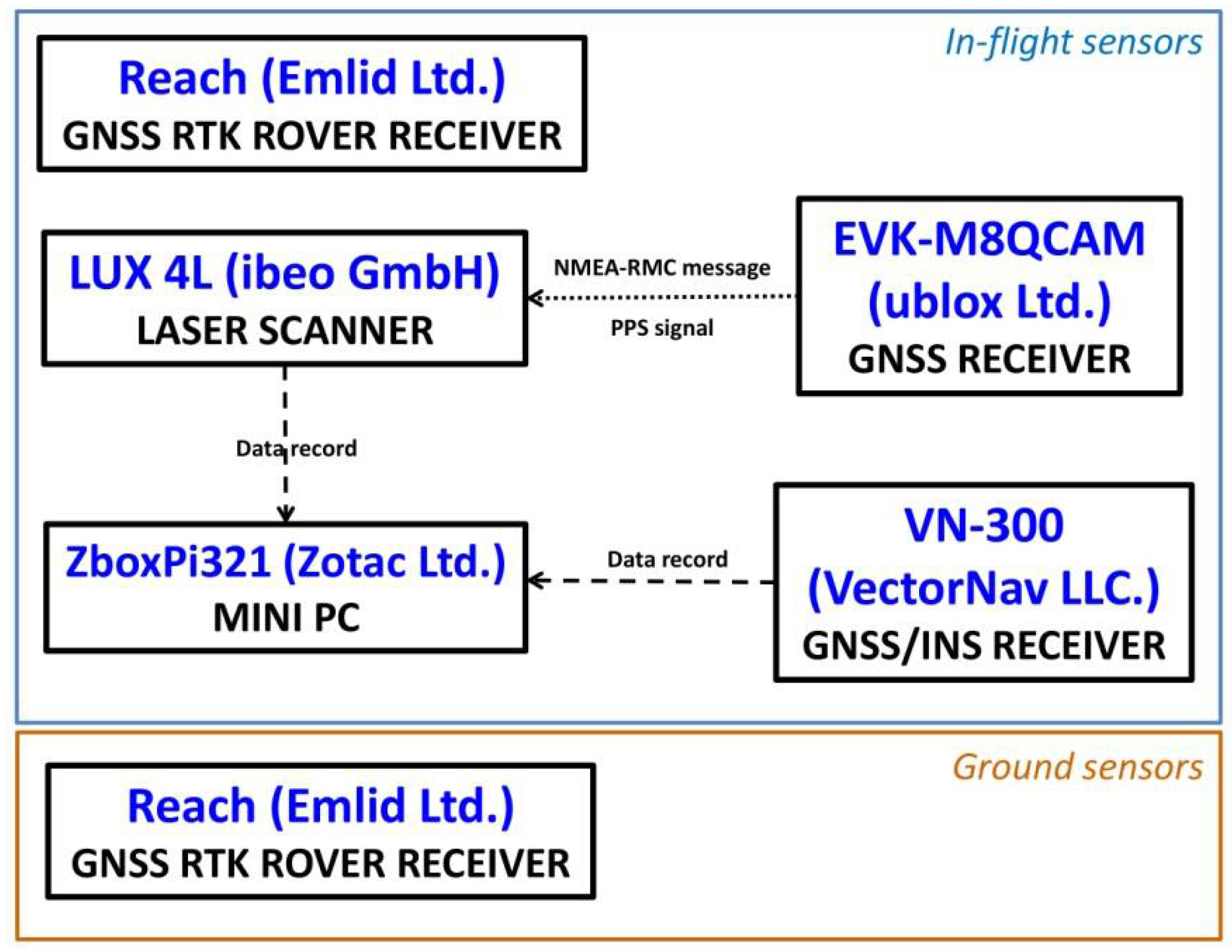
The resulting architecture of the system is shown in Figure 2. The GNSS time from the EVK-M8QCAM is sent to the LUX 4L, VN-300 data are recorded in the mini PC by means of a Python [17] script, and Reach receiver data are directly registered in the record card of the rover and base modules.

All integrated components of the LiDAR system are protected inside a polycarbonate box, which is installed on a rigid frame. To reduce transmitted shock and vibration from UAV rotors, the frame is connected to the UAV body using silicone rubber vibro-insulators selected according to the weight and vibration frequency of the UAV propellers.

The weight of all sensors, including antennas, reached 1.5 kg, meeting the requirements of the maximum take-off weight of the UAV used to carry the laser scanner system, which is 5.5 kg (batteries included). The UAV, which was designed and developed by engineers involved in the project, has 12 brushless motors, a hexa-coaxial configuration, and a mono frame in polyamide powder sinterized by means of selective laser sintering (SLS). It has a stand-alone control system and an onboard navigation system, so it is able to autonomously fly via uploaded waypoints. From the hardware side, there are two electronic circuit boards. One, the flight control (FC) board (Mikrokopter Flight Ctrl V2.5), is responsible for flight dynamics and mode setup by the remote pilot. The other, the navigation control (NC) board (Mikrokopter Navi Ctrl V2.1), is responsible for managing the UAV position when the GPS mode is set up. The operating mode by the GPS allows the UAV to follow the predefined position. Whether or not the UAV is not unsettled by the pilot, the NC orders the FC to maintain the current position. Whether or not a way point and information about the route distance covered is uploaded before the flight, in automatic mode, the UAV follows the consecutive points of the waypoint list. In this case, information about height and speed are also uploaded in the NC. Flight time of the UAV is around 10 min, with a payload of 5 kg. Data acquisition can be controlled from the ground by means of Wi-Fi remote control.

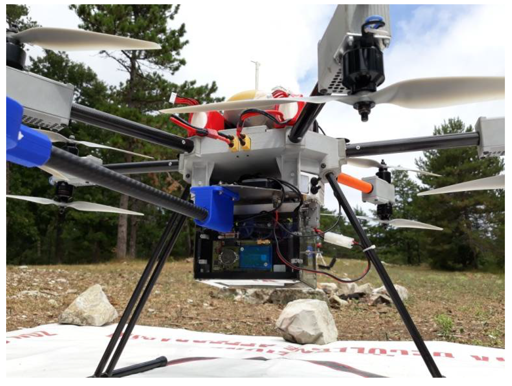
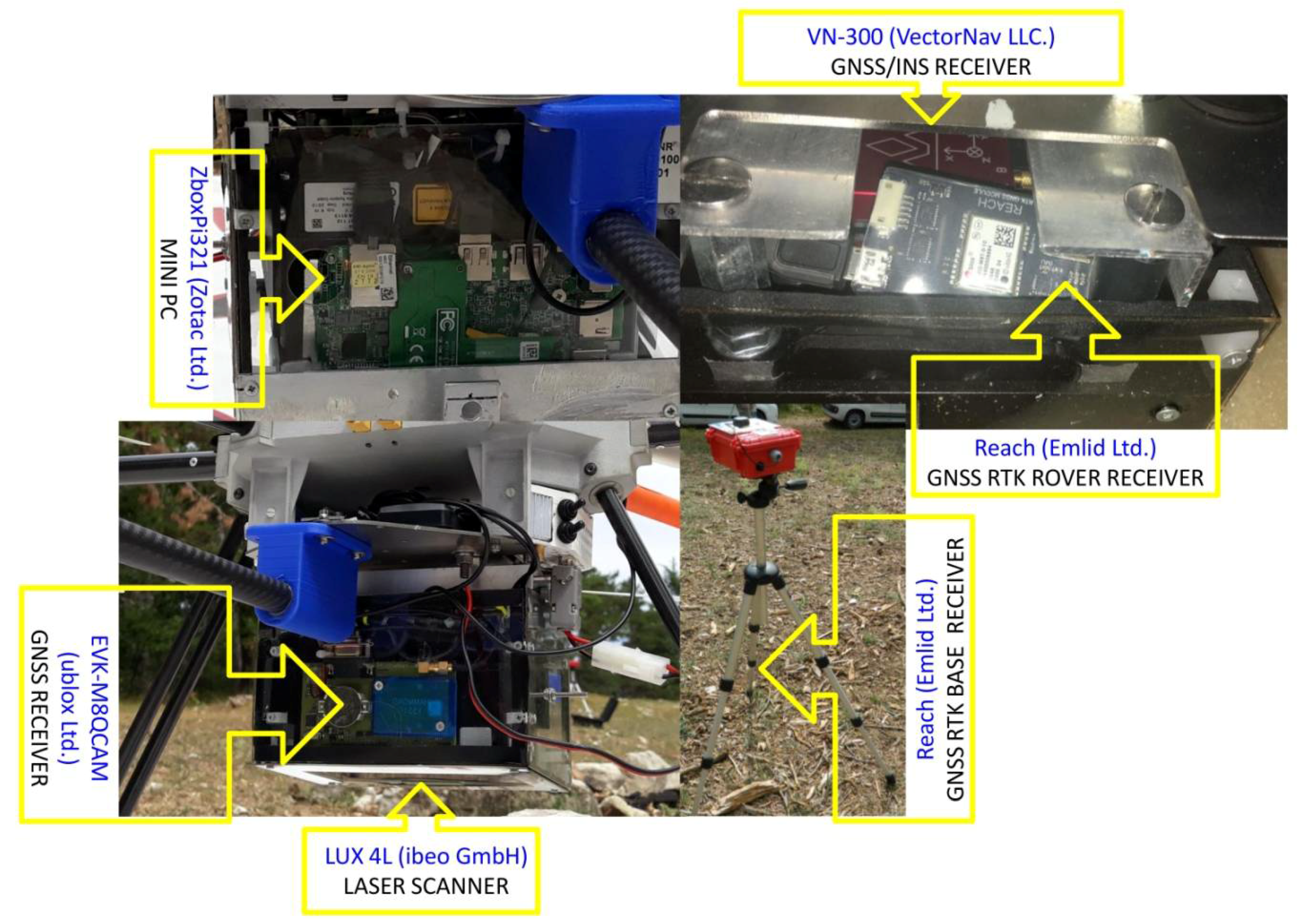
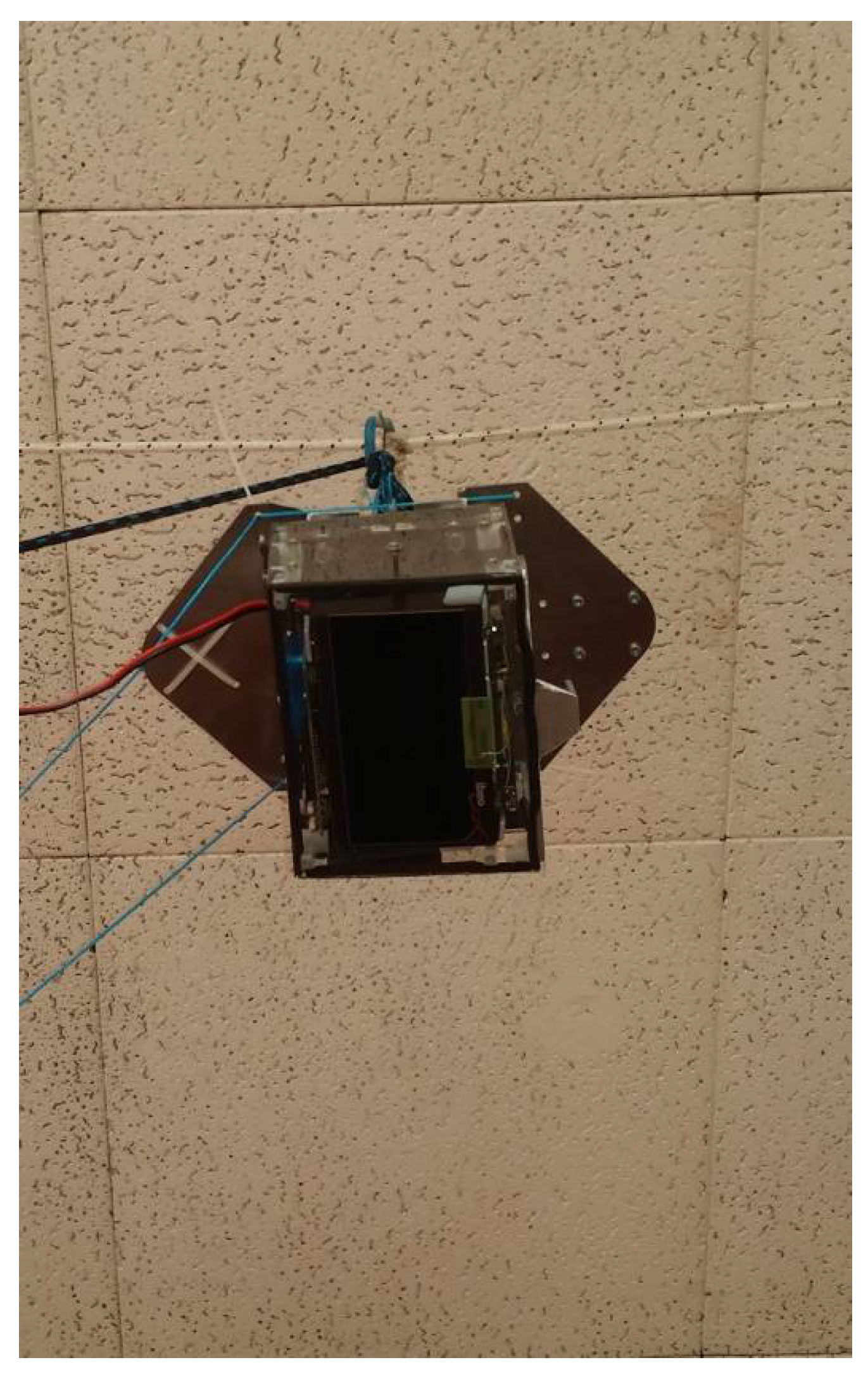
The LiDAR system mounted in the UAV in operating conditions is illustrated in Figure 3, while Figure 4 shows each sensor integrated in the system.

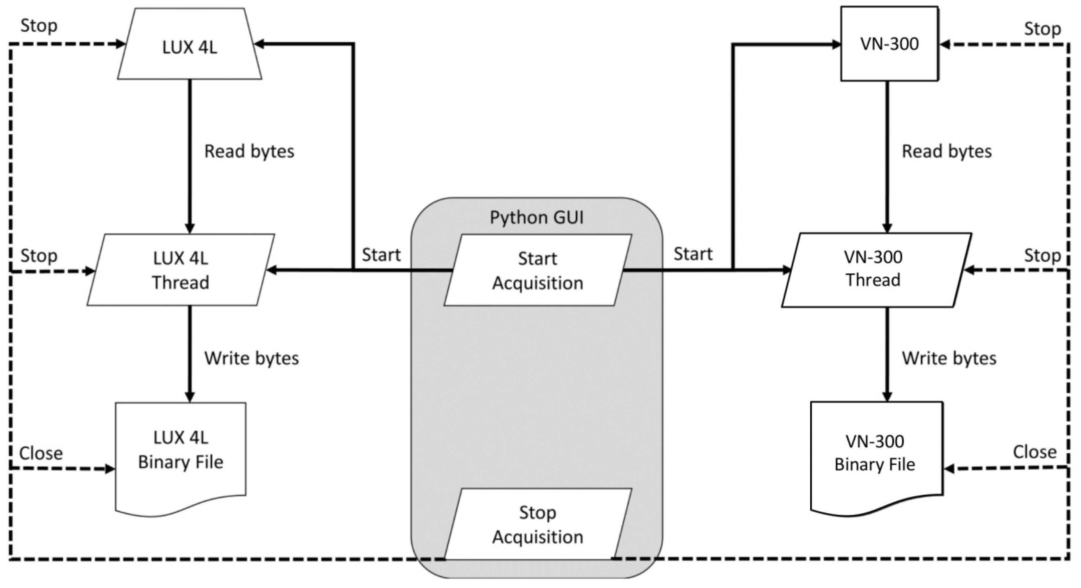
For the acquisition of laser scanner LUX 4L and GNSS/INS VN-300 data, a script in Python was developed. The script runs beneath a simple graphical user interface (GUI) that allows the user to start and stop the acquisition process. When the acquisition is started, the application sends a specific message to both the LUX 4L and the VN-200, triggering the beginning of the measurements, and therefore the data stream, from the instruments to the computer. The application then spawns two threads that make use of simple socket functions to read and write a certain number of bytes in a binary file, which is closed when the user ends the acquisition through the GUI. When the acquisition ends, the read-write threads are closed and specific stop messages are sent to the instruments to halt the data stream (Figure 5).

2.2. Data Postprocessing and LiDAR Point Cloud Generation

In postprocessing, laser scanner and INS binary data are decoded to a readable format via decoding routines. The laser scanner data are decoded in MATLAB (MathWorks Inc., Natick, MA, USA), and two files are generated by this process, one with the data about the laser pulses and one with the data about the returns. The INS data are first parsed by proprietary software (Binary Output Configuration Tools, VectorNav Technologies LLC, USA), and the output, still in binary format, is decoded in MATLAB. The GNSS RTK data are differentially corrected in postprocessing using RTKLIB [17], an open source program package for GNSS positioning.

Once the data have been decoded, the next phase is the LiDAR point cloud generation. The first step is to interpolate the yaw, pitch, and roll based on the time of INS and latitude, longitude, and altitude based on the time of the GNSS RTK receiver to the time of the laser pulse transmission. In this way, a matrix with the laser scanner points and the associated position and orientation of the LiDAR sensor is generated. The second step is to generate the LiDAR point cloud by means of the LiDAR equation [18], which was adapted considering that the laser scanner acquires in four parallel layers. The position of the laser point is derived through the summation of three vectors after applying three appropriate rotation matrixes [18]. The position of each return was calculated using Equation (1):

$${\overrightarrow{\mathrm{X}}}_{\mathrm{G}}={\overrightarrow{\mathrm{X}}}_0+{\mathrm{R}}_{\mathsf{\omega },\mathsf{\varphi },\mathsf{\kappa }}{\mathrm{R}}_{\mathsf{\Delta }\mathsf{\omega },\mathsf{\Delta }\mathsf{\varphi },\mathsf{\Delta }\mathsf{\kappa }}{\overrightarrow{\mathrm{P}}}_{\mathrm{G}}+{\mathrm{R}}_{\mathsf{\omega },\mathsf{\varphi },\mathsf{\kappa }}{\mathrm{R}}_{\mathsf{\Delta }\mathsf{\omega },\mathsf{\Delta }\mathsf{\varphi },\mathsf{\Delta }\mathsf{\kappa }}{\mathrm{R}}_{\mathsf{\alpha },\mathsf{\beta }}\left[\begin{array}{c}0\\ 0\\ -\overrightarrow{\mathsf{\rho }}\end{array}\right]$$

(1)

where ${\overrightarrow{\mathrm{X}}}_{\mathrm{G}}$ represents the ground coordinates of the return; ${\overrightarrow{\mathrm{X}}}_0$ represents the ground coordinates of the GNSS RTK antenna phase center; ${\overrightarrow{\mathrm{P}}}_{\mathrm{G}}$ is the offset between the laser scanner and the GNSS RTK antenna phase center with respect to the laser scanner coordinate system (lever-arm offsets); and $\overrightarrow{\mathsf{\rho }}$ is the laser range vector, whose magnitude is equivalent to the distance from the laser firing point to its target. The term ${\mathrm{R}}_{\mathsf{\omega },\mathsf{\varphi },\mathsf{\kappa }}$ stands for the rotation matrix relating the ground and INS coordinate systems; ${\mathrm{R}}_{\mathsf{\Delta }\mathsf{\omega },\mathsf{\Delta }\mathsf{\varphi },\mathsf{\Delta }\mathsf{\kappa }}$ represents the rotation matrix relating the INS and laser unit coordinate systems (bore-sighting angles); and ${\mathrm{R}}_{\mathsf{\alpha },\mathsf{\beta }}$ refers to the rotation matrix relating the laser unit and laser beam coordinate systems, with α and β being the mirror scan angles [18].

The lever-arm offset between the laser scanner and the GNSS RTK antenna phase center was measured in the laboratory. As the INS was mounted corresponding to the point of laser beam emission, it was not necessary to measure the lever-arm offset between the laser scanner and the INS.

2.3. Measurement Uncertainty Estimation Approaches and Setups

The International Vocabulary of Metrology (VIM) [19] defines measurement uncertainty as a “non-negative parameter characterizing the dispersion of the quantity values being attributed to a measurand, based on the information used.” Measurement uncertainty expresses incomplete knowledge about the measurand, hence a probability distribution over the set of possible values for the measurand can be used to represent the corresponding state of knowledge about it. This probability distribution “expresses how well one believes one knows the measurand’s true value” and fully characterizes how the degree of this belief varies over that set of possible values. For scalar measurements, the standard deviation (σ) is the attribute of this probability distribution that represents its scatter over the range of possible values. This property of repeated measurements is referred to as precision. When the true value of the measurand is known, the closeness of agreement between a measured quantity value and a true quantity value can be assessed, and it is defined as accuracy.

As a measure of accuracy, the root mean-squared error (RMSE) was calculated to compare the measured value (${\widehat{\mathrm{y}}}_{\mathrm{i}}$) with the true value (${\mathrm{y}}_{\mathrm{i}}$), as follows:

$$\mathrm{RMSE}=\sqrt{\frac{{{\displaystyle \sum }}_{\mathrm{i}=1}^{\mathrm{n}}{\left({\widehat{\mathrm{y}}}_{\mathrm{i}}-{\mathrm{y}}_{\mathrm{i}}\right)}^2}{\mathrm{n}}}$$

(2)

where n is the number of measurements.

Besides the RMSE, the mean absolute error (MAE) was also computed, as in Equation (2), because according to [20], this dimensioned statistic is a more natural measure of average error:

$$\mathrm{MAE}=\frac{1}{\mathrm{n}}{\displaystyle \sum }_{\mathrm{i}=1}^{\mathrm{n}}|{\widehat{\mathrm{y}}}_{\mathrm{i}}-{\mathrm{y}}_{\mathrm{i}}|$$

(3)

In this framework, three setups were considered, as reported in

Table 2. Three setups to assess the accuracy of LasUAV components and parameters to characterize uncertainty. RMSE, root mean-squared error; MAE, mean absolute error.

Type of Scenario/Setup	Component of LasUAV under Assessment	Parameters Characterizing Uncertainty and Error
S1: Angular static	Laser scanner	σ, RMSE, MAE
S2: Angular dynamic	Laser scanner + INS	σ, RMSE, MAE
S3: In-flight	Laser scanner + INS + GNSS RTK	σ

, to assess the uncertainty and the accuracy coming from the three sensors of the LasUAV. By the angular static setup (scenario 1, S1) and the angular dynamic setup (scenario 2, S2), the uncertainty and accuracy attributable to the laser scanner and to the laser scanner and INS, respectively, were quantified. By the in-flight setup (scenario 3, S3), the uncertainty attributable to all sensors of the LasUAV was assessed.

2.4. Angular Static and Dynamic Setups: Laser Scanner and INS Measurement Uncertainty Analysis

In angular static and dynamic conditions, to characterize the uncertainty in planimetric measurements, (X,Y) is difficult because the LasUAV is an aerial system geared to near-nadir flight. For this reason, only uncertainty in elevation measurements (Z) originating from the laser scanner in S1 and S2 was assessed.

According to Equation (1), three variables originating from the laser scanner are included in the LiDAR equation: the distance from the point of emission of the laser beam ($\overrightarrow{\rho })$, which is dynamic, i.e., it changes in time during the scanning; the laser scan angle ß, which is dynamic; and the layer transversal beam divergence angle α, which is fixed, i.e., it does not change. Angles ß and α are assumed to be correct, since they are related to the physical design of the instrument and to the geometric alignment of the laser sensor and the scanning mirrors. Distance measured by the laser scanner may be impacted by the accuracy of the time measurement of each pulse. For these reasons, the uncertainty in Z measurements of the laser scanner was assessed keeping the LasUAV in a stationary position pointing to a flat surface located at a known distance of 317.0 cm (Figure 6), measured by the DISTO D2 laser distance meter (Leica Geosystems AG, , Heerbrugg, Switzerland).

According to Equation (1), the INS provides values of the yaw, pitch, and roll to be imputed in the LiDAR equation. In S2, angular dynamic conditions were generated by varying the pitch and roll of the LasUAV, pointing to the same flat surface located at the same known distance, in the range of +3° and −3°, which corresponds to the typical range in operational flight conditions on multirotor UAV platforms.

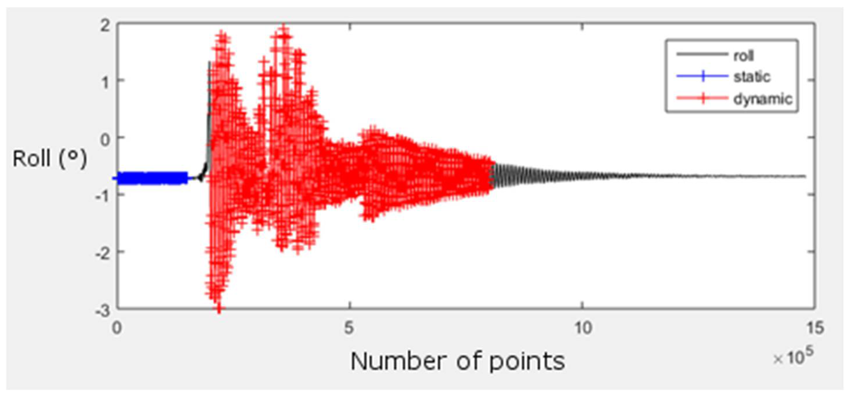
For S1 and S2 setups, we started from the assumption that in both cases, with LasUAV stationary and moving, the floor is horizontal and flat. The standard deviation and MAE of Z represent the uncertainty and accuracy, respectively, of the laser scanner or the uncertainty and accuracy of the laser scanner and INS when data from both sensors are coupled.

Two subsets were generated from the same acquisition and used to assess the uncertainty in angular static and dynamic conditions (Figure 7).

2.5. In-Flight Setup: Laser, INS, and GNSS RTK Measurement Uncertainty Analysis

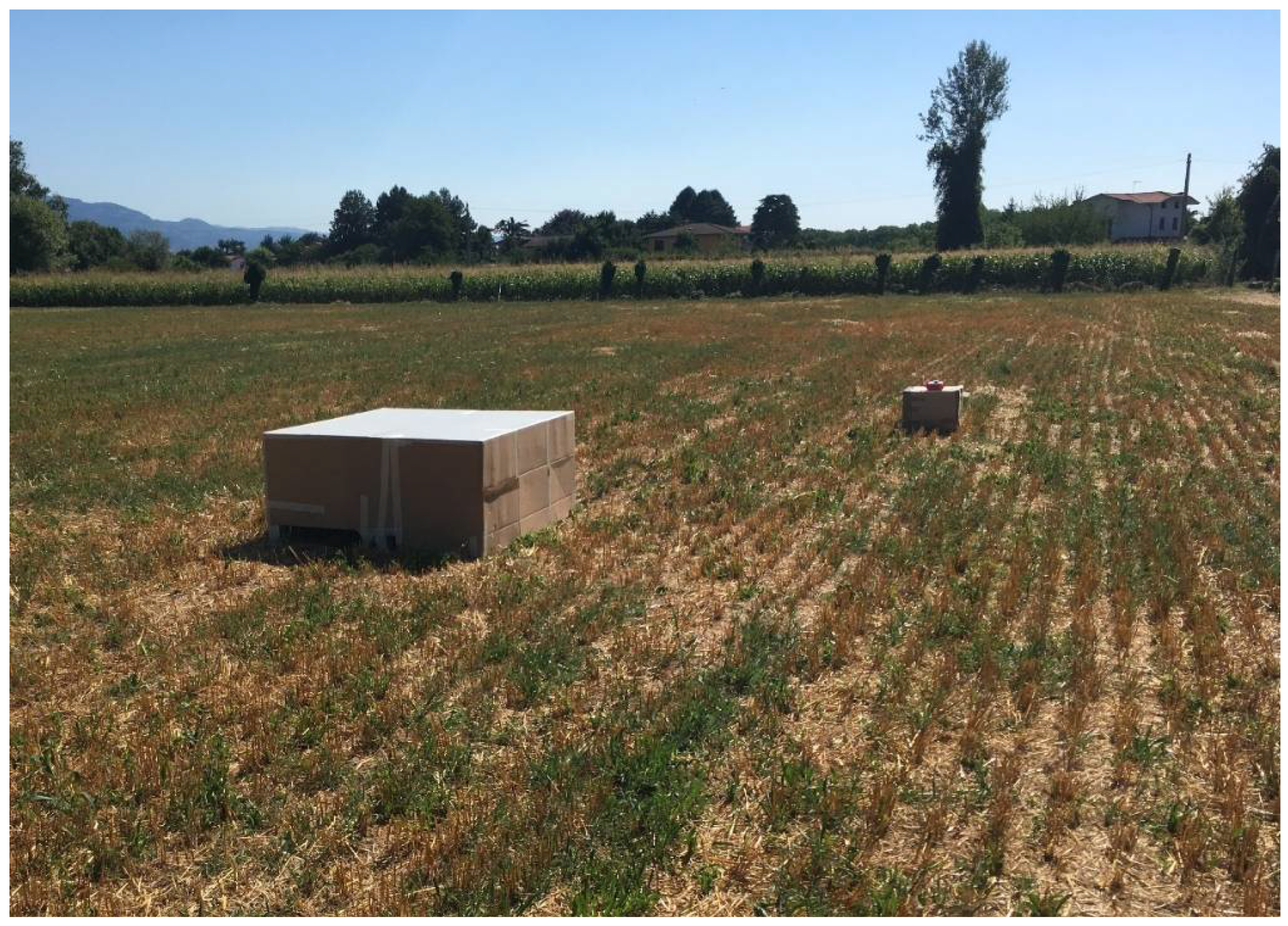
In S3, the in-flight setup, the uncertainty of the LasUAV was assessed through an analysis using datasets from the test field composed of the control surface of a box. The components of the LasUAV system under investigation with this setup were the laser scanner, the INS, and the GNSS RTK receiver. This setup allowed the assessment of three sources of uncertainty: (i) uncertainty in Z associated with a single passage over the target; (ii) uncertainty in Z associated with multiple passages (from one to nine) over the target; and (iii) uncertainty in the horizontal positioning of X and Y of the target associated with multiple passages (from one to nine).

A flat area of 10,000 m² with a box as a target was sampled with an automatic flight at an average flying height of 10 m (HFOV = 11.55 m) and horizontal velocity of 2 m/s^–1 (Figure 8).

The LasUAV traveled through the area, scanning the target in nine repeated passages. For each passage over the target, an analytical procedure was developed to extract subsets of the entire point cloud corresponding to individual passages and to spatially locate the target. The position of the target at each flight passage, represented by a rectangle coincident with the top of the box, was determined within each point cloud with an optimization procedure; the actual position was computed among all the possible positions as the one that minimized the sum of residuals (a residual being the difference between the elevation value of each point falling inside the rectangle and the true elevation of the top of the box). For the cloud points falling inside the rectangle representing the top of the box, the mean and the standard deviation of Z were computed.

An analysis of possible combinations of one passage (i.e., nine combinations of one passage from the set of nine passages), two passages (36 combinations of two passages from the set of nine passages), three passages (84 combinations of three passages from the set of nine passages), four passages (126 combinations of four passages from the set of nine passages), five passages (126 combinations of five passages from the set of nine passages), six passages (84 combinations of six passages from the set of nine passages), seven passages (36 combinations of seven passages from the set of nine passages), eight passages (nine combinations of eight passages from the set of nine passages), and nine passages (one combination of nine passages from the set of nine passages) was conducted to assess the variation in uncertainty in Z in the case of UAV flights made with multiple passages, i.e., to assess the overall variability of the target position among multiple passages, related to the positioning accuracy of the system. Uncertainty was calculated as the average value of the standard deviation of all possible combinations for each set of passages. For example, in the combination of two passages over the nine passages in the set, uncertainty was calculated as the mean of 36 values of standard deviation; in the combination of three passages over the sample of nine passages in the set, uncertainty was calculated as the mean of 84 values of standard deviation, and so on. This analysis allows us to understand how many passages over the area of interest made in a UAV campaign can affect the overall uncertainty of the point cloud.

3. Results

The results from angular static and dynamic test activities that allowed calculation of the MAE and standard deviation associated with Z measurements (σ_z) are reported in

Table 3. Results of the uncertainty and accuracy assessment of LiDAR height measurements in angular and static dynamic conditions.

Type of Acquisition	Number of Points	σZ (cm)	MAE (cm)	RMSE (cm)
S1: Angular static	150,000	3.8	3.9	5.5 cm
S2: Angular dynamic	600,000	3.9	3.7	5.3 cm

. The MAE and standard deviation of height measured have small differences between angular static and dynamic conditions.

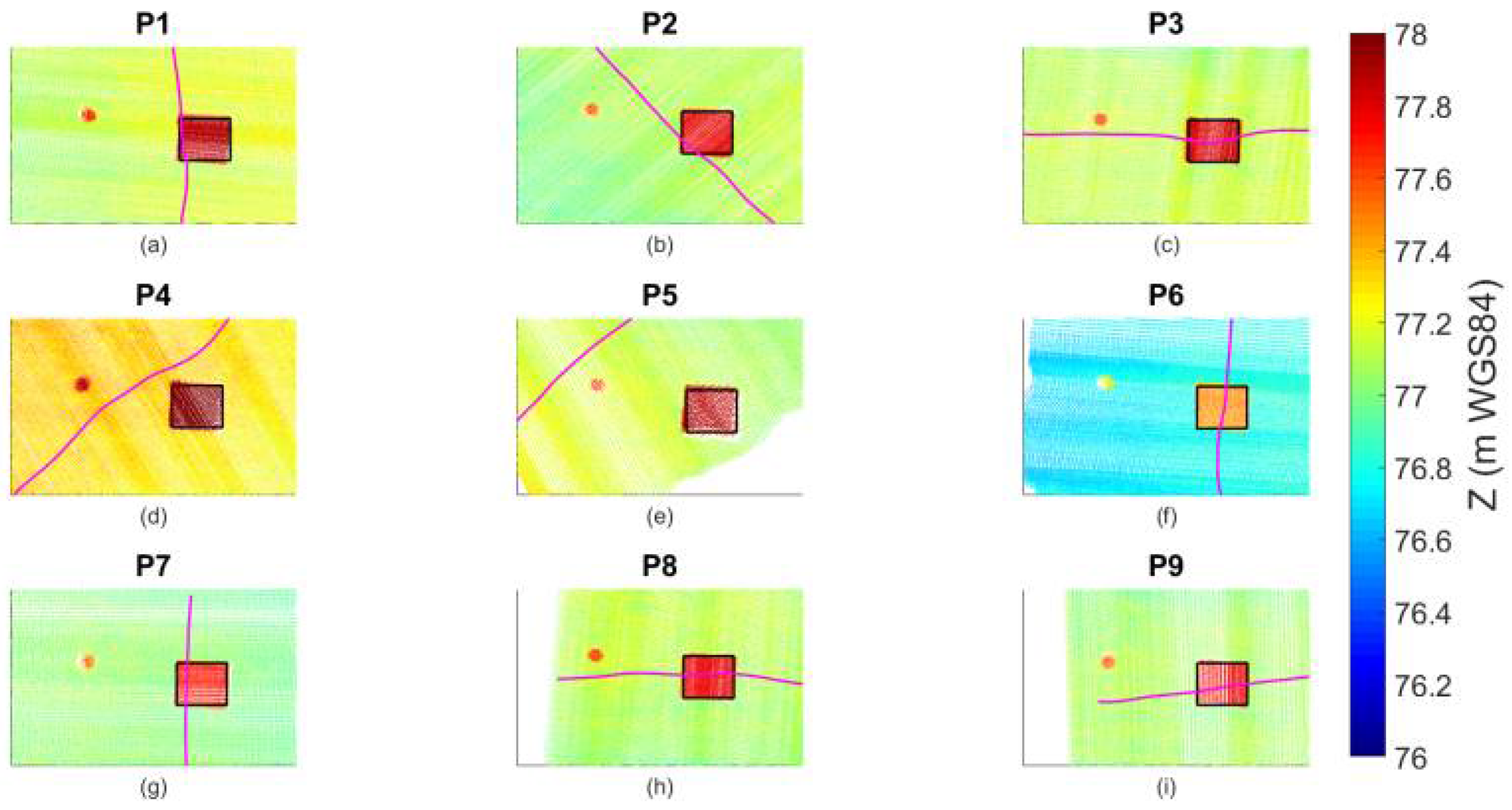
Figure 9 illustrates the point cloud from each of the nine passages during the flight.

As we can see from Figure 9, the target was reached from laser pulses with different track orientations and laser beam angulations. For example, for P4 and P5, the scan was moderately and largely decentralized, respectively, with respect to the box, and for this reason, the target was hit sideways; for P1, P2, and P7, the scans were slightly decentralized with respect to the target; while for P3, P6, P8, and P9, the box was hit most by laser pulses oriented near-nadir.

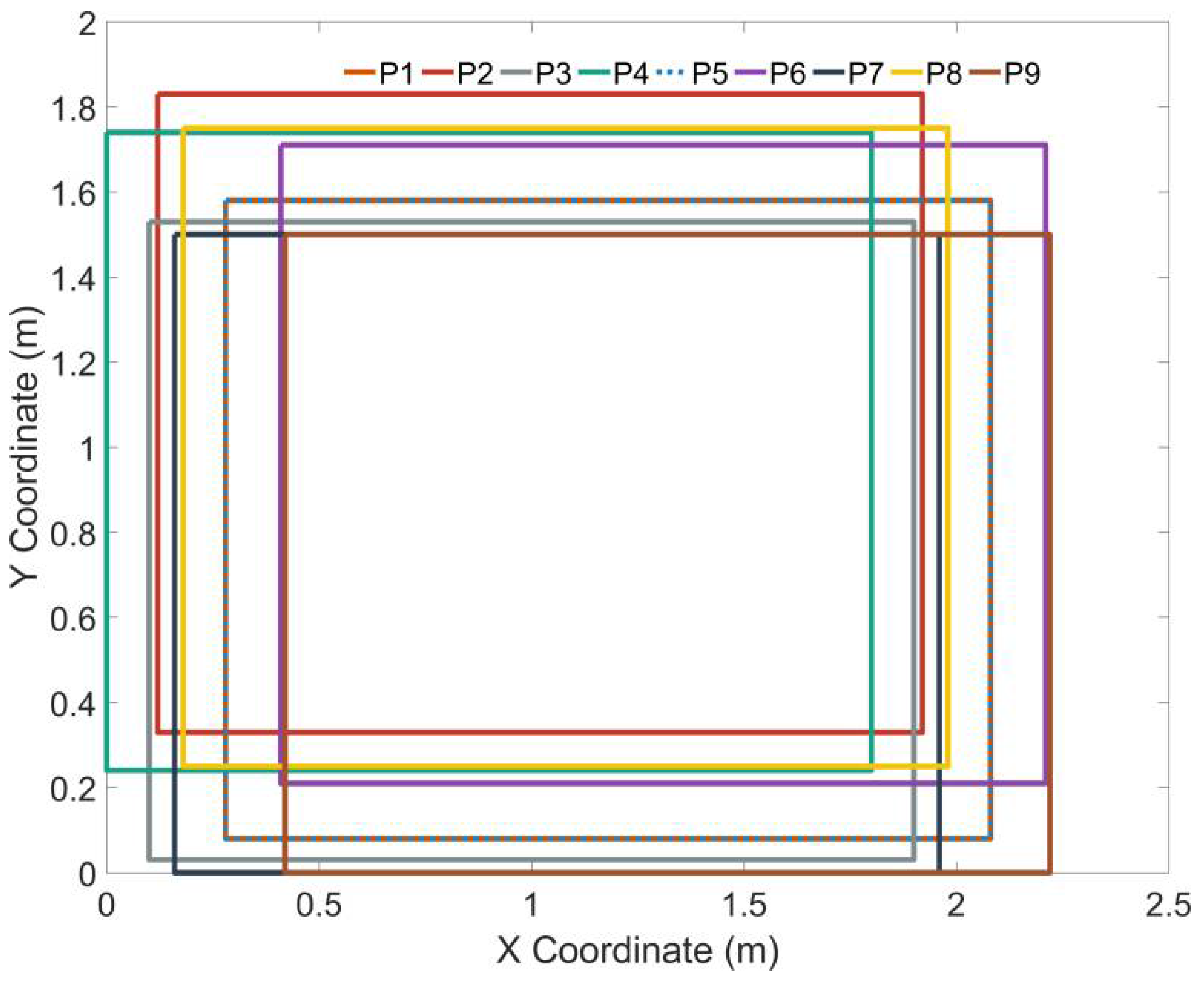
Figure 10 shows the horizontal positions colored with different tones of the target identified in each of the nine passages.

The results of the uncertainty analysis in in-flight conditions are reported in

Table 4. Results of the uncertainty assessment of LiDAR height measurements in in-flight conditions. X and Y are the offset (in m) between the lower left angle of the target and the origin indicated in Figure 6.

Passage	Roll (°)	Yaw (°)	Number of Points	X (m)	Y (m)	Z (m)	σZ (cm)
P1	−4.95	4.2	1583	0.28	0.08	77.85	5.7
P2	−5.44	−39.47	1290	0.12	0.33	77.75	6.7
P3	0.58	98.49	1405	0.10	0.03	77.79	6.1
P4	10.57	−121.28	1382	0.00	0.24	78.02	9.8
P5	−23.62	58.35	866	0.28	0.08	77.85	7.3
P6	−0.66	4.92	1068	0.41	0.21	77.43	9.2
P7	5.68	−179.02	867	0.16	0.00	77.69	5.7
P8	0.79	−86.38	1537	0.18	0.25	77.75	5.1
P9	−0.39	88.76	791	0.42	0.00	77.73	7.5

. For each passage, the mean values of scan angle and yaw are reported with the number of returns in the cloud. X and Y are the mean coordinates of the left down edge of the top of the box with respect to the origin of the relative reference system, while Z is the mean ellipsoidal height of the box cover.

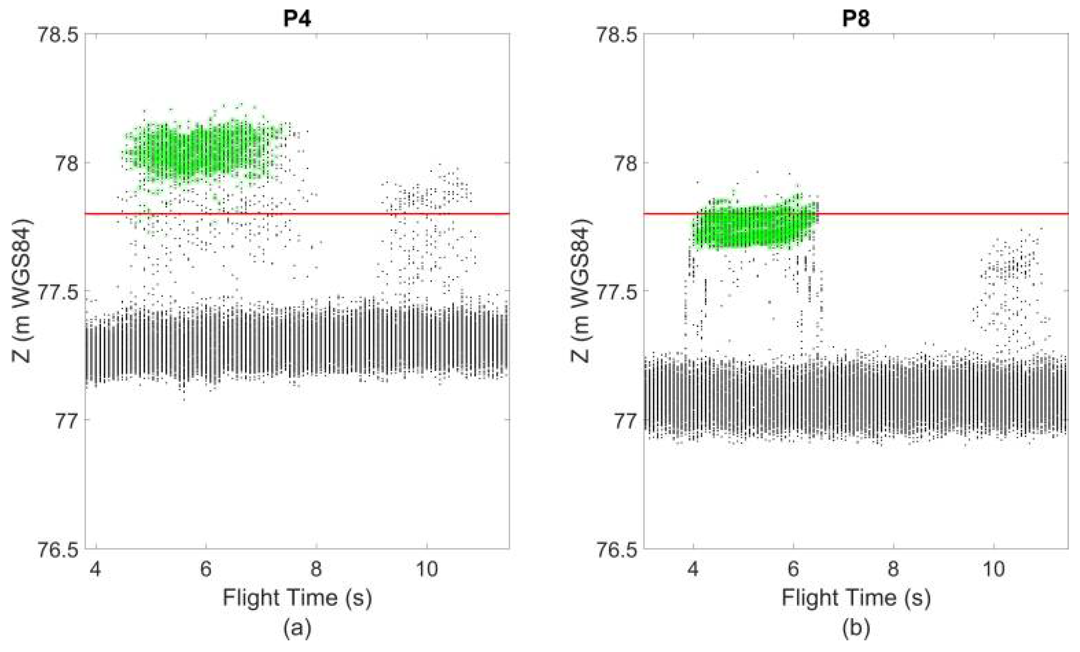
In the nine passages, P4 had the worst standard deviation (σ_Z = 9.8 cm), which corresponds to the highest value of uncertainty. This is due to the poor results from the differential corrections as a consequence of a weak GNSS signal, which determines the worsening target identification and increased dispersion. This case can be considered an outlier. On the contrary, P8 represents the passage with the lowest uncertainty (σ_Z = 5.1 cm). Figure 11 shows the returns that hit the cover of the box in passages P4 and P8. In P4, the cover is positioned at a height higher than expected; this is not interpretable as a bias (understood as a systematic difference between population mean of the measurement results and the accepted reference value), but as uncertainty due to unstable values of the GNSS signal.

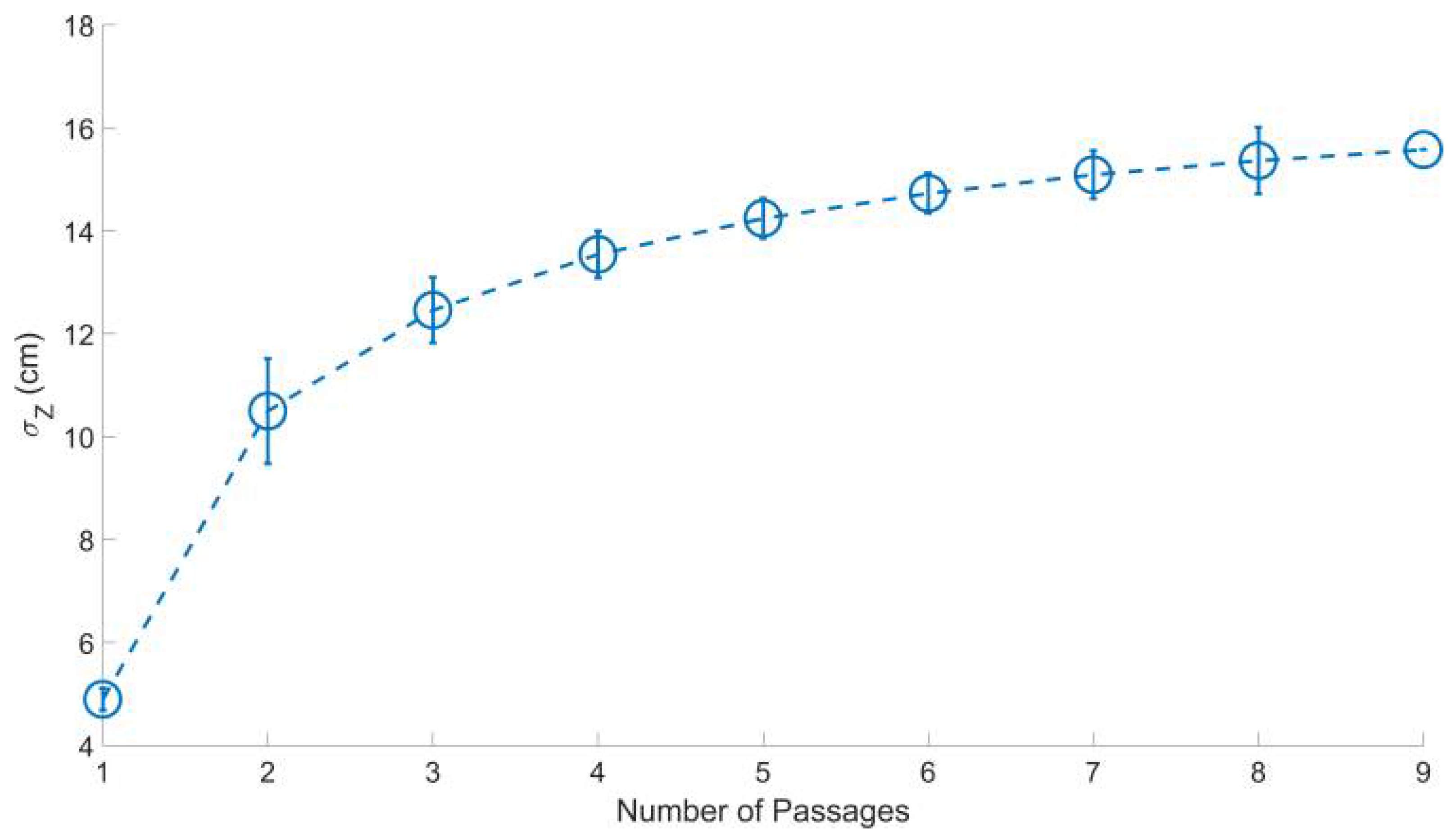
Figure 12 represents the results from the analysis of possible combinations of passages; the uncertainty in Z is represented as a function of the number of multiple passages over the target. In the case of a single passage, uncertainty has the lowest value and its standard deviation is the lowest. In the case of nine passages, uncertainty reaches the highest value but its standard deviation is the lowest. This means that there is a trend in the uncertainty of one passage toward nine passages.

Summarizing, uncertainty in Z in angular static conditions is equal to 3.8 cm, which increases to 3.9 cm in angular dynamic conditions. Uncertainty in Z in in-flight conditions ranges between 5.1 cm and 9.8 cm, while in multiple passages, obtained as a combination of nine single passages, it ranges between 5 cm and 16 cm.

4. Discussion

In this paper, the motivation and technical details of developing the LasUAV are described, and its performance is assessed in terms of accuracy and partitioning among multiple error sources.

All the major error sources were independently considered by means of analysis made in both angular static and dynamic conditions, and in in-flight conditions.

With respect to other studies that tested UAV LiDAR systems developed for agriculture or forestry application, the first and basic assessment of the performance of the LasUAV was conducted in controlled conditions and on a target with a simple geometric shape whose dimensions were exactly measured and whose state was not affected by external conditions, such as wind.

In fact, for example, [13] assessed the effect of high-density point clouds (up to 62 returns/m²) produced by the UAV-LiDAR system on the measurement of location, height, and crown width of isolated trees. In this case, the standard deviation of tree height was 0.15 m, the standard deviation of tree location was 0.53 m, and the standard deviation of crown was 0.61 m. The assessment of reproducibility of the relative height distribution of 3D point-cloud data from the laser system developed by [14] was conducted in a rice paddy; they found that mapping accuracy was 1.56 ± 0.12 m without ground control point (GCP) correction and 0.23 ± 0.10 m using only one GCP. The UAV mapping system for agricultural field surveying designed by [15] was tested in crop volume estimates calculated using a voxel grid of the canopy heights of crop biomass with a spatial resolution of 0.04 m × 0.04 m × 0.001 m.

In contrast to the above-mentioned studies, whose tests allowed assessment of the total uncertainty of the system, the study presented here allowed us to quantify the uncertainties associated with the different subcomponents of the system and their impact on total uncertainty.

The uncertainty and MAE in Z of the LasUAV had small differences between angular static and dynamic conditions. In angular static and dynamic conditions, in the uncertainty scales with a distance from the target from 3 m to 10 m (i.e., typical flight altitude), there is no significant variation, because the measurement error scale is trigonometric. For this reason, the uncertainty at a 3 m distance is small and at 10 m is still not sizable. This means that if the laser scanner system is used at low heights over the target surface, an INS with high values in angular static and dynamic (pitch/roll) accuracy is not needed. These figures changed in in-flight conditions, where the uncertainty in Z of the measurements of LasUAV ranged between 5.1 cm and 9.8 cm for single passages, during which the target was reached from laser pulses with different angulations (ranging from near-nadir to very far-nadir). For the combination of nine passages, uncertainty ranged between 5 cm and 16 cm. In other words, uncertainty in a small number of passages (one or two) is dominated by uncertainty coming from both the laser and the GNSS RTK receiver, whereas for an increasing number of passages (three to nine), uncertainty becomes dominated by the GNSS RTK receiver. This allows us to conclude that if the user of the laser scanner system is interested in the lowest values of uncertainty, a single passage over the area of interest is recommended. This could be the case of UAV-borne laser scanner campaigns over wide forest areas with the goal of scanning the maximum surface in the shortest time. For UAV-borne laser scanner campaigns with repeated passages, the positioning uncertainty coming from the GNSS is in the running and the duration of the flight. In general, this kind of flight survey method is to be avoided, because if the GNSS signal reception is moving away from good conditions of acquisition, the uncertainty in Z measurements will increase markedly. In fact, the longer the flight duration, the higher the probability of a leap in the GNNS calculated position, due, for example, to an abrupt satellite constellation change. This allows us to conclude that the GNSS RTK sensor mostly influences the uncertainty of laser measurements. Consequently, a strong effort should be put into selection of the GNSS RTK, and a bigger economic investment should be devoted to this sensor.

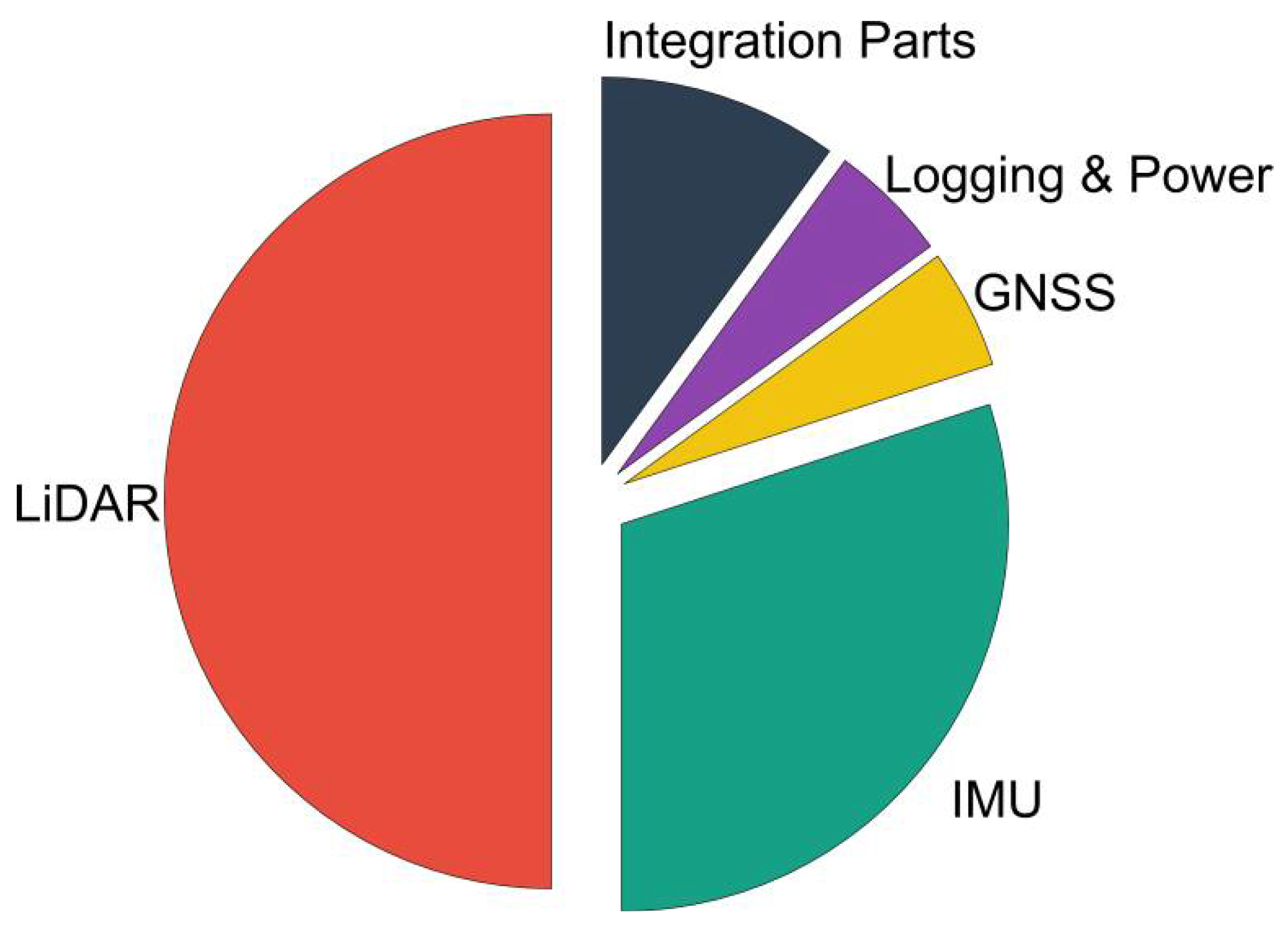
The new LasUAV is a low-cost laser scanner system; its hypothetical selling price (20,000 €) would be lower than the price of the two most commonly used commercial all-integrated LiDAR systems for forestry application. From the hardware point of view, the relative incidence of each component in the total cost of the LasUAV is illustrated in Figure 13. The laser scanner is the sensor that most influences the cost (~10,000 €, 50%), followed by the INS (~6000 €, 30%), then the integration parts (2000 €, 10%), and finally the GNSS RTK receiver (~1000 €, 5%) and the logging and power (~1000 €, 5%).

The levels of uncertainty in Z measurements in in-flight conditions of our LasUAV are comparable to those achieved by typical airborne laser scanners [2,3] and are similar to those obtained by [13] (RMSE of the point cloud against ground control point equal to 0.34 m, standard deviation of tree height equal to 0.15 cm).

LasUAV will provide efficiencies for projects and create new opportunities in areas such as linear corridors, dense vegetation, and steep mountains. In UAV laser scanning, the inherent direct georeferencing workflows do not require, for example, the redundancy required in many UAV photogrammetric workflows. Processing data to infer terrain is more straightforward if using an appropriate LiDAR sensor, and in mountainous areas, being able to reduce dependency on ground control points reduces on-site risk.

The growing popularity of low-cost UAVs is resulting in the development of miniaturized laser scanner devices and GNSS RTK receivers increasingly at a low cost, which the forestry sector and other disciplines such as plant physiology and phenotyping will take advantage of. As a matter of fact, laser scanning from a system such as LasUAV allows data acquisition for the accurate digital three-dimensional reconstruction of canopies. Variables originating from LiDAR data, such as leaf density, leaf angle, and curvature, can capture differences in canopy architecture and can be used to quantify actual photosynthetic productivity, which is usually difficult to estimate in complex canopies, partly because of a lack of high-resolution canopy structural data [21]. The integration of such data will establish links between vegetation structure, function, and physiology and consequently, will generate more accurate photosynthetic productivity estimation models.

5. Conclusions

This paper describes the development of a UAV laser scanner system, including the process for generating 3D point clouds based on the precise UAV position and orientation. The integration of a GNSS RTK receiver with a dual-antenna GNSS-aided INS is an efficient solution to provide sufficient accuracy for forest monitoring applications by means of laser scanning.

The performance assessment of the system was conducted in a point cloud obtained from scans over targets with a controllable and measurable geometry.

The experiments conducted and the analyses carried out allow us to conclude that LiDAR point cloud uncertainty is most influenced by the GNSS RTK sensor, and for this reason, the biggest economic investment should be dedicated to this sensor.

In addition, specific analyses accomplished in the combination of passages made over the target allowed us to conclude that a single passage over the area of interest is recommended to reach the lowest values of uncertainty and maximize the surface scanned over wide forest areas.

Future improvements of LasUAV will include inserting a filter to screen interactions between the dual antenna of GNSS-aided INS and the UAV rotors, and using novel batteries to increase flight endurance and avoid frequent take-offs and landings.

Future studies will address assessing the performance of the system in forest surveying. Understanding the added value of a UAV-borne laser scanner system, such as LasUAV, with respect to the airborne laser scanner system, is important for making decisions in forest monitoring, management, and planning.