Assessing Ecosystem Isoprene Emissions by Hyperspectral Remote Sensing

Abstract

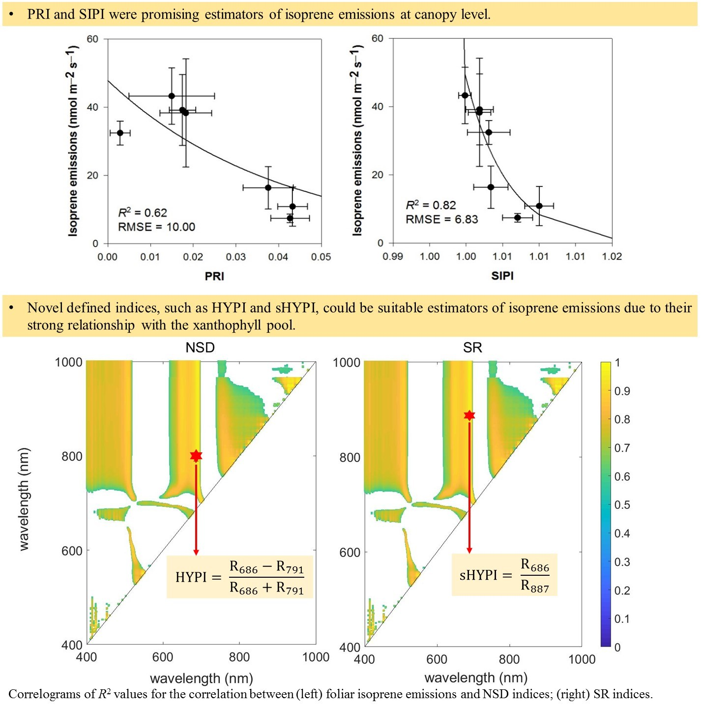
This study examined the relationship between foliar isoprene emissions, light use efficiency and photochemical reflectance index (PRI) throughout the canopy profile and explored the contribution of xanthophyll cycle pigments versus other carotenoid pigments to the isoprene/PRI relationship. Foliar isoprene emissions within the canopy profile were measured in a high-density poplar plantation in Flanders (Belgium) during the 2016 growing season. The results confirmed that PRI was a promising estimator of isoprene emissions at canopy level. Interestingly, xanthophyll cycle pigments contributed more to isoprene biosynthesis than chlorophyll and drove the isoprene/PRI relationship. The simple independent pigment index and novel defined indices, such as the hyperspectral isoprene index and simple hyperspectral isoprene index, showed promising results and could be suitable estimators of isoprene emissions due to their strong relationship with the xanthophyll pool.

1. Introduction

Plants are an important source of biogenic volatile organic compounds (BVOC) with about 1150 Tg C yr⁻¹ emitted by plants to the atmosphere globally and 500 Tg C yr⁻¹ emitted as isoprene [1]. The emission of isoprene has a large impact on the Earth’s atmospheric composition and climate because of its high reactivity in the troposphere [2]. In particular, the presence of isoprene in the atmosphere alters the NO–NO₂–O₃ cycle, responsible for O₃ formation–degradation [3] leading to the formation of other secondary pollutants, such as peroxyacyl nitrates and particulate matter [4].

Isoprene emissions from an ecosystem can either be directly quantified at the foliar level through cuvette measurements or indirectly at the canopy level. Currently, ecosystem level monitoring sites are scarce worldwide; therefore, the quantification of isoprene emissions at the canopy level is far from being resolved with the available models and field measurements [5]. The widely used Model of Emissions of Gases and Aerosols from Nature (MEGAN model ) [6] incorporates the instantaneous responses of emissions to changes in radiation fluxes and foliar temperature within the canopy, and to factors representing the influence of past conditions of temperature and radiation, the effect of soil-moisture stress and the leaf age estimated using the leaf area index. The parameterization of the emission inhibition due to soil-moisture stress depends on such limited information as soil-water moisture, which has led to contradictory findings across various models [7].

The seasonal variability of isoprene emissions can be determined by the application of remotesensing techniques for the detection of formaldehyde [8] or by detectable changes in foliar carotenoid concentrations. A strong relationship has been reported between foliar isoprene emissions and the photochemical reflectance index (PRI) [9,10], a remotely sensed vegetation index based on the leaf xanthophyll cycle and on the leaf chlorophyll/carotenoids ratio [11,12]. The combined use of this index with a model, such as MEGAN, can lead to better predictions of foliar isoprene emission variability [5]. The direct comparison of ecosystem isoprene emissions with information derived from remotely sensed vegetation indices has been recently investigated by using PRI derived from Moderate Resolution Imaging Spectroradiometer (MODIS) satellite data [13]. Two previous studies investigated the use of PRI to quantify isoprene emissions, but both were performed under controlled environmental conditions on small potted poplar shoots [5,14]. Further information is needed to fully understand the applicability of the isoprene/PRI relationship for scaling up foliar information to an ecosystem scale. In this regard there is a need to clarify the role of xanthophyll versus carotenoids in the PRI signals related to isoprene emissions [13]. In this study, we, therefore, aimed to better understand the relation between foliar isoprene emissions, light use efficiency (LUE) and PRI throughout the canopy profile and the contribution of pigment pools to the isoprene/PRI relationship under natural environmental conditions.

2. Materials and Methods

2.1. Field Study Site and Sampling Protocols

All measurements were performed at an existing field site in Lochristi, Belgium (51°06′44″N 3°51′02″E) at an elevation of 6 m a.s.l. The intensively cultured poplar plantation was established in 2010 (http://uahost.uantwerpen.be/popfull/) and consisted of 12 poplar (Populus) genotypes planted in monoclonal blocks with a tree density of 8000 cuttings ha⁻¹. An exhaustive description of the study site and its management as well as of the poplar materials has been previously published [15,16]. Poplars (Populus) are strong emitters of isoprene, as observed in canopy-scale studies for this plantation [17,18], with an annual return of assimilated carbon in the form of isoprene at around 0.3% [19]. This study focused on the growing season of the year 2016, the third and last year of the third rotation after the coppice in early 2014. Foliar measurements were made between mid-July and the end of August 2016 in correspondence with the maximum growth period and to the peak of isoprene emissions [19]. Four field campaigns were performed during sunny (photosynthetically active radiation, PAR ≥ 900 μmol m⁻² s⁻¹) days. Among the genotypes at the plantation, one of the most productive and strongest isoprene emitters, genotype Skado (Populus trichocarpa × Populus maximowiczii), was selected for measurements [17]. Five shoots per genotype were selected and their vertical canopy profile sampled: 5 shoots × 2 heights (adult leaves at 3.5 m and at the top of the canopy at 8 m) × 2 leaves at each height, i.e. 20 samples in total, where the photosynthetic capacity, associated isoprene emissions, and hyperspectral reflectance were measured.

2.2. Measurements of Photosynthetic Capacity and Light-Use Efficiency

All measurements at foliar level were made between 11:00 a.m. and 2:00 p.m. (CET), because isoprene emissions and PAR were highest at midday [17,19]. The leaf photosynthetic capacity (A_max, µmol m⁻² s⁻¹) was measured with a portable CO₂/H₂O exchange system (LI-6400, LI-COR, Lincoln, NE, USA) by clamping leaves in a 6 cm² cuvette. The instrument was set-up with the same parameters as proposed in earlier studies [17,20]. The cuvette air flow rate was 400 µmol s⁻¹ and the CO₂ concentration inside the cuvette was kept at 400 ± 4 µmol mol⁻¹. The LI-6400 was set to a PAR of 1000 µmol m⁻² s⁻¹, a block temperature of 25 °C and a vapor pressure deficit of 1.07 ± 0.03 kPa. Reflectance was measured immediately after A_max on the same leaves. We calculated LUE as the ratio between A_max and the incident PAR reaching each leaf. Foliar samples were then collected for pigment extraction.

2.3. Measurements of Isoprene Emissions

While A_max was being measured, the air exiting the leaf cuvette was routed to fill a 0.6 L Tedlar sampling bag (model 30284-U Supelco, Eighty Four, PA, USA) equipped with a screw cap valve and a Thermogreen septum. The gas exchange cuvette was flushed with VOC-free air previously scrubbed with a charcoal filter (Supelco, Eighty Four, PA, USA) placed ahead of the inlet [17]. Within one hour after collection the air in each bag was flushed to a quadrupole-based proton-transfer-reaction mass spectrometer (PTR-MS) (Ionicon, Innsbruck, Austria) for at least 10 s at a rate of ~2 Hz, and the concentration of isoprene of at least 20 data points in the time series was averaged. The PTR-MS instrument was calibrated before every field campaign. The reaction rate of isoprene within the PTR-MS was assessed with a gas mixture containing a known concentration of isoprene, which had been transferred to a Tedlar bag for one hour. This practice did not only accurately calibrate the instrument to calculate the isoprene concentration in the air sample, but it also included the possible influence of the bag on the isoprene concentration stability, even if the bag material was the most suited to contain VOC due to its inert surfaces. The isoprene concentration measured in the sampling bags was transformed to a foliar isoprene emission rate (Φ_isoprene, nmol isoprene m⁻² s⁻¹) using the following equation:

$${\Phi }_{isoprene}=\frac{C_{isoprene} \times Q_{cuvette}}{A_{cuvette}}$$

(1)

where C_isoprene is the concentration of isoprene in the sample bag (ppbv), Q_cuvette is the molar flow rate of the cuvette (mol s⁻¹) and A_cuvette is the area of the leaf enclosed in the LI-COR cuvette (m²).

2.4. Measurements of Hyperspectral Reflectance

Foliar hyperspectral reflectance was measured over the spectral region between 350 and 1600 nm (2-nm sampling interval) by coupling an ASD FieldSpec FR Pro spectroradiometer (ASD, Boulder, CO, USA) with a leaf clip. Hemispherical reflectance was derived as the ratio of reflected to incident radiance. Each reflectance spectrum was automatically calculated and stored by the spectroradiometer as an average of 20 readings. Dark current was measured before starting each spectral sampling. These measurements were done immediately after the leaf photosynthetic and isoprene measurements. We calculated PRI [9], which has been demonstrated to be a good proxy of isoprene emissions. Furthermore, PRI is sensitive to changes in LUE and xanthoplyll cycle activity. The foliar spectral response at 531 nm, a spectral band that correlated with diurnal changes of LUE, is affected by conversions of xanthophyll cycle pigments between their epoxidized and de-epoxidized states. The idea to use PRI in predicting foliar isoprene emissions is based on the inverse relationship between isoprene emissions and LUE. Foliar photosynthetic activity is reduced when LUE is low and consequently more reducing power for isoprene production is available. Many studies have reported that isoprene emissions are related to carotenoid content [21,22]. The existence of the relationship between isoprene emissions and carotenoids is based on either substrate availability or complementary functionality. We therefore calculated the structural independent pigment index (SIPI) [10], a proxy of carotenoid/chlorophyll ratio, in addition to PRI to test this hypothesis. We calculated SIPI using the spectral reflectance at 445 nm, which corresponds to the carotenoid absorption peak, and reflectance in the red region (680–800 nm), which is related only to chlorophyll.

$$\mathrm{PRI}= \frac{{\mathrm{R}}_{531}-{\mathrm{R}}_{570}}{{\mathrm{R}}_{531}+{\mathrm{R}}_{570}}$$

(2)

$$\mathrm{SIPI}= \frac{{\mathrm{R}}_{800}-{\mathrm{R}}_{445}}{{\mathrm{R}}_{800}+{\mathrm{R}}_{680}}$$

(3)

where R is the reflectance at the selected wavelength band (nm).

In order to explore the use of hyperspectral data for estimating isoprene emissions, and LUE, we performed a correlation analysis between the two spectral reflectance indices (PRI or SIPI as independent variables) and these (isoprene emissions and LUE) dependent variables.

Additionally, we calculated simple spectral ratio (SR) and normalized spectral difference (NSD) indices using all possible combinations of two-band (i and j) reflectance (R) between 400 and 1000 nm (180, 600 combinations).

$$\mathrm{SR}= \frac{{\mathrm{R}}_i}{{\mathrm{R}}_j}$$

(4)

$$\mathrm{NSD}= \frac{{\mathrm{R}}_i-{\mathrm{R}}_j}{{\mathrm{R}}_i+{\mathrm{R}}_j}$$

(5)

Linear regression analyses were performed among all possible wavelength combinations for SR and NSD and the investigated dependent variable (i.e., isoprene emissions). The performance of linear models in predicting the dependent variables was evaluated by the coefficient of determination (R²) and the root mean square error (RMSE). The linear models used log-transformed values of isoprene emissions. The NSD and SR with highest R² were selected as the best indicators of isoprene emissions. In particular, we defined NSD as HYPI (HYPerspectral Isoprene) index and SR as sHYPI (simple HYPerspectral Isoprene) index. A Pearson’s correlation analysis was performed (see Section 2.6 for more details).

2.5. Pigment Analyses

Foliar samples were collected immediately after the reflectance measurements, immediately frozen in liquid N₂ in the field, and then stored at −80 °C. Pigments were extracted and analyzed by high-performance liquid chromatography (HPLC) using a 1260 Infinity chromatograph (Agilent Technologies, Santa Clara, CA, USA) as described by Thayer and Björkman [23] to determine the foliar pigment concentrations. The HPLC system was calibrated using commercial pigment standards.

Xanthophyll-cycle pigment pools (VAZ) were determined as the sum of violaxanthin (V), antheraxanthin (A) and zeaxanthin (Z) concentrations. Total carotenoids (Car) were determined as the sum of VAZ, neoxanthin (N), lutein (L), and β-carotene (b) concentrations. Total chlorophyll (Chl) was determined as the sum of chlorophyll-a and -b concentrations. Carotenoid pigment levels were normalized to Chl levels. The epoxidation state (EPS) of the xanthophyll cycle was expressed as:

$$\mathrm{EPS}= \frac{\mathrm{V}+0.5\times \mathrm{A}}{\mathrm{V}+\mathrm{A}+\mathrm{Z}}$$

(6)

2.6. Statistical Analyses

We applied exponential regression models and a correlation analysis to investigate the relationships between the vegetation indices, the rate of foliar isoprene emissions and LUE.

We built linear models with the predictors of isoprene emissions (i.e., PAR, PRI and canopy position) to evaluate how much of the variability of isoprene emissions could be explained by combinations of predictors. The canopy position predictor took into account the leaf age and structure. The linear models used log-transformed values of isoprene emissions. We conducted a univariate analysis for each variable to determine the correlation between each predictor and isoprene emissions. We used a single linear regression for continuous variables and one-way analysis of variance (ANOVA) with post hoc Tukey’s honest significance difference (HSD) tests for categorical variables. We performed stepwise backward regression analysis (SBRA) by considering all variables together and successively removing the least important variable that did not pass a multicollinearity test, i.e. with a variance inflation factor > 5. The original model was compared with a new model with one variable removed using the likelihood ratio and the Akaike information criterion. The new model was not accepted if the likelihood ratio increased.

Finally, we performed the Pearson linear correlation analysis to investigate the roles of xanthophyll-cycle pigments and other carotenoid pigments in the vegetation indices linked to isoprene emissions. All statistical analyses used R statistical software (version 3.1.2).

3. Results

3.1. Canopy Profile of Foliar Isoprene Emissions, Light Use Efficency and Photochemical Reflectance Index

Overall, adult leaves at the top of the canopy (8 m) emitted more isoprene (38.5 ± 4.5 nmol m⁻² s⁻¹, average ± SE) than leaves positioned at the lowest level of 3.5 m (11.4 ± 4.5 nmol m⁻² s⁻¹). Of the incoming PAR that reached the top of the canopy (1526 ± 213 µmol m⁻² s⁻¹) only about 23% reached leaves positioned at 3.5 m (355 ± 221 µmol m⁻² s⁻¹). Leaf temperature was slightly lower in leaves at the lower level (25.6 ± 0.8 °C) compared to the upper level (26.5 ± 1.7 °C).

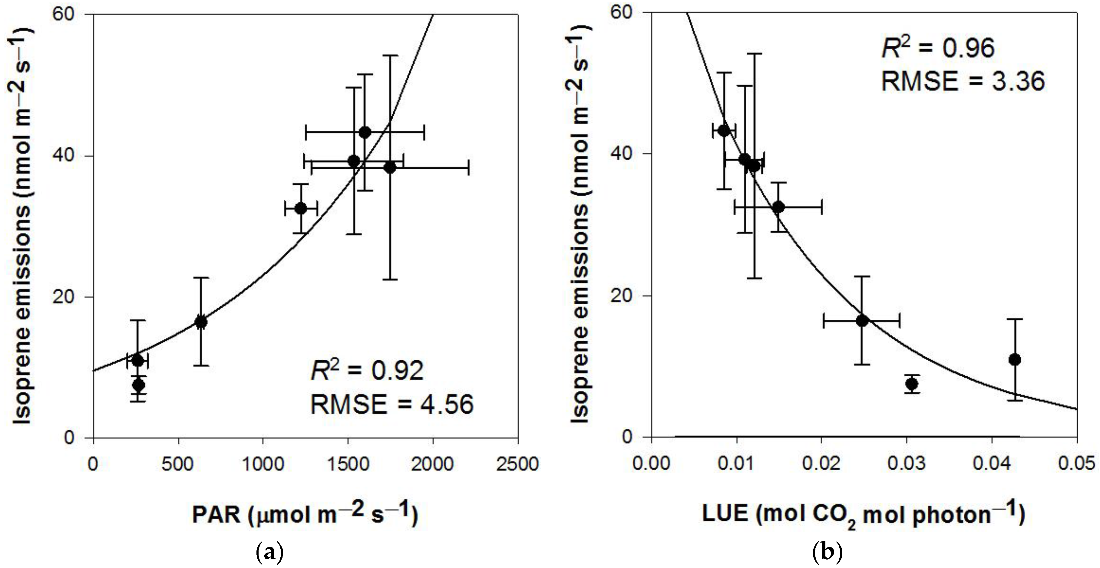
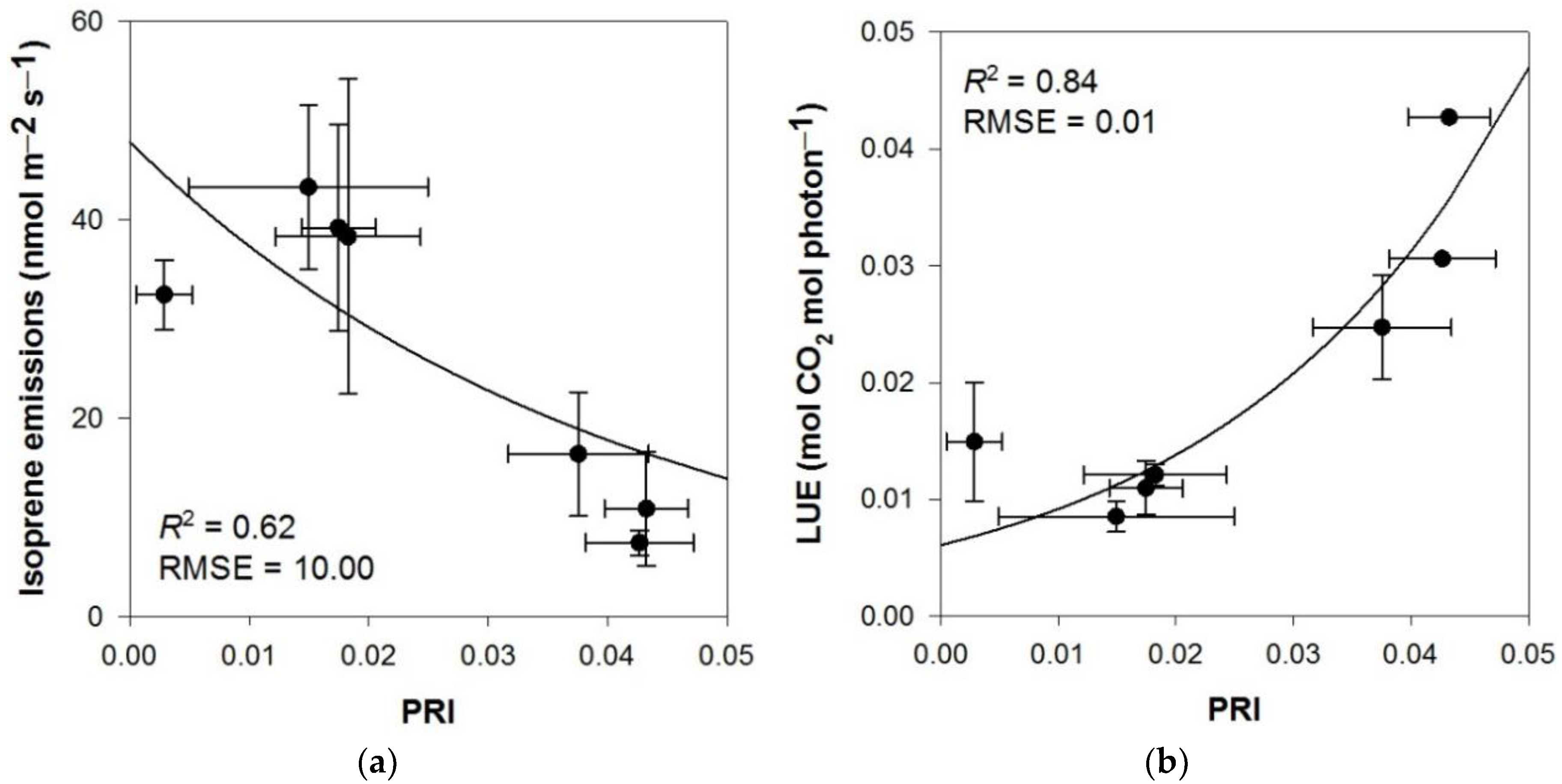
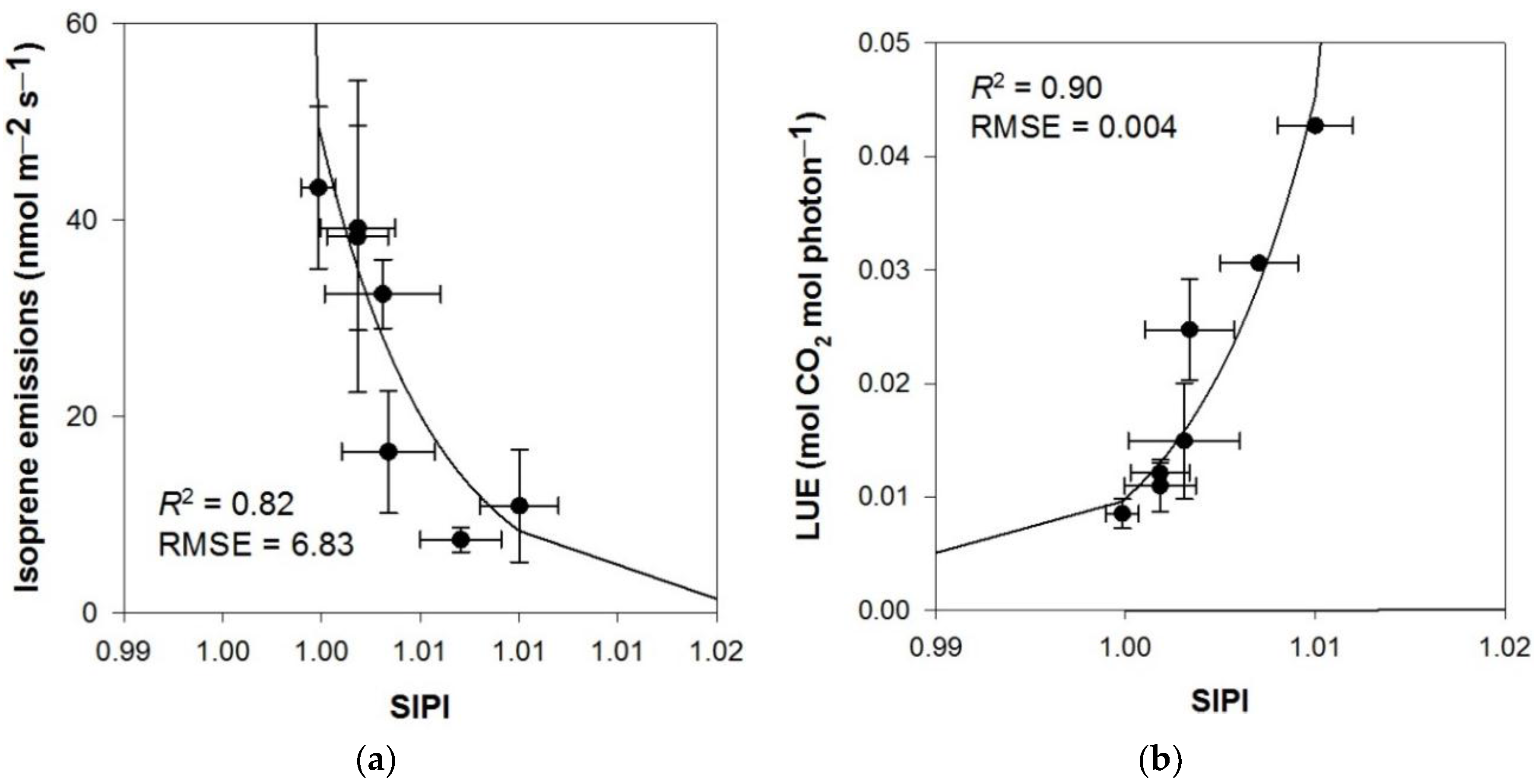
Foliar isoprene emissions were exponentially correlated (R² > 0.92) with both PAR (Figure 1a) and LUE (Figure 1b). PRI also correlated exponentially with foliar isoprene emissions (Figure 2a) and with LUE (Figure 2b). Results of linear correlation analyses between log-transformed foliar isoprene emissions, PAR and PRI are presented in

Table 1. Impact of photosynthetically active radiation (PAR), photochemical reflectance index (PRI) and leaf position on isoprene emissions reflected from univariate analysis and stepwise backward regression analysis (SBRA). Level of significance of the linear regression (p) and R² are reported for the continuous variables. The results of a one-way ANOVA (p) and a post-hoc Tukey’s HSD test (absolute difference for two significantly different factors and p of the difference) is reported for the categorical variable. The variables of the final SBRA model, indicated with X and representing the key predictors of isoprene emissions, and R² for the final model are reported.

Predictor	Univariate Analysis			SBRA
	Variable Type	R2 (p)	Post-Hoc (p)	R2 (p)
PRI	continuous	0.78 (0.008)		X
PAR	continuous	0.94 (<0.001)		X
Leaf position	categorical		(0.002)
Stepwise backward regression				0.95 (0.002)
Model

. A significant linear relationship between log-transformed isoprene emissions and PAR was found (R² = 0.94; p < 0.01). Also, PRI showed a significant linear relationship with log-transformed isoprene emissions. Considering PAR, PRI and canopy position as predictors in only one model, SBRA analysis on the same dataset produced a model with a high value of R² = 0.95 (Table 1). Only PAR and PRI showed a significant correlation, while canopy position—that was related to leaf age and structure—did not have significant importance. Foliar isoprene emissions and LUE were highly correlated (R² = 0.82 and 0.90, respectively) to SIPI (Figure 3) following exponential functions.

3.2. Exploring Novel Vegetation Indices to Predict Isoprene Emissions

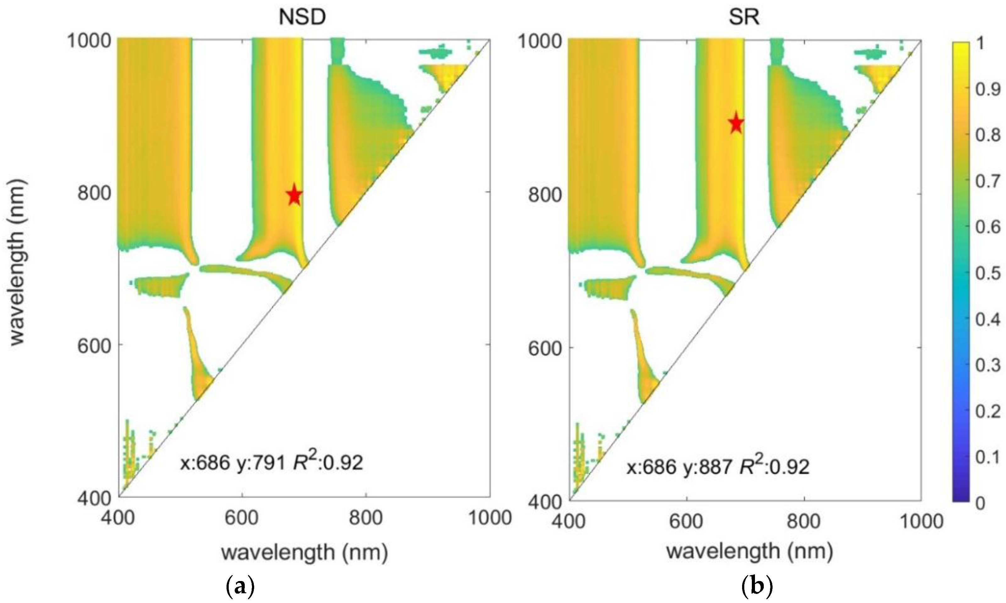
As expected, the correlograms returned the highest correlation values in the spectral band region of PRI around 531 nm and 570 nm (Figure 4). Interesting insights may be gained from the two correlograms. Both the NSD and SR indices are highly correlated in the same spectral regions. The correlations were strongest either for indices combining bands in the visible range (VIS < 700 nm) or at the red end of the spectrum into the near infrared (NIR > 700 nm), corresponding to spectral regions used by indices such as PRI and the water-band index (WI), respectively. Spectral regions of well-known indices, such as the normalized vegetation index (NDVI), SR and SIPI, that exploit the contrasting reflectance magnitudes in the visible and NIR, had slightly lower correlations with isoprene emissions. Combining bands for pigments between 400 and 520 nm and NIR bands (between 780 and 1000 nm) in particular produced good correlations.

3.3. Relationship between Foliar Pigments and Vegetation Indices

The VAZ/Chl ratio showed the highest correlation (r = 0.97) with foliar isoprene emissions (

Table 2. Pearson correlation coefficients of investigated variables: log(isoprene emissions) = logarithm of isoprene emissions (nmol m⁻² s⁻¹); PRI; SIPI; HYPI = hyperspectral isoprene index; sHYPI = simple hyperspectral isoprene index; Car = total carotenoids; Chl = total chlorophylls; Car/Chl = total carotenoids/total chlorophylls ratio; N/Chl = neoxanthin/chlorophyll ratio; V/Chl = violaxanthin/chlorophyll ratio; A/Chl = antheraxanthin/chlorophyll ratio; Z/Chl = zeaxanthin/chlorophyll ratio; L/Chl = lutein/chlorophyll ratio; b/Chl = β-carotene/chlorophyll ratio; VAZ = xanthophyll-cycle pigment pools; EPS = epoxidation state. Correlation coefficients with p < 0.05 are shown in bold.

	Log (Isoprene Emissions)	PRI	SIPI	HYPI	sHYPI	Car	Chl	Car/Chl	N/Chl	V/Chl	A/Chl	Z/Chl	L/Chl	b/Chl	VAZ/Chl	VAZ	EPS
Log (isoprene emissions)	1
PRI	−0.88	1
SIPI	−0.87	0.75	1
HYPI	−0.96	0.97	0.83	1
sHYPI	−0.96	0.97	0.83	1.00	1
Car	−0.11	0.27	0.37	0.23	0.23	1
Chl	−0.29	0.47	0.47	0.42	0.42	0.97	1
Car/Chl	0.40	−0.39	−0.03	−0.40	−0.39	0.73	0.54	1
N/Chl	−0.80	0.91	0.82	0.91	0.91	0.58	0.72	−0.05	1
V/Chl	0.86	−0.80	−0.89	−0.85	−0.85	−0.38	−0.53	0.19	−0.81	1
A/Chl	0.92	−0.94	−0.76	−0.93	−0.93	−0.06	−0.25	0.44	−0.80	0.70	1
Z/Chl	0.68	−0.63	−0.27	−0.66	−0.65	0.49	0.29	0.86	−0.32	0.35	0.73	1
L/Chl	−0.03	0.01	0.26	−0.01	−0.01	0.63	0.53	0.79	0.22	0.01	−0.09	0.42	1
b/Chl	0.40	−0.52	−0.03	−0.49	−0.48	0.57	0.38	0.92	−0.22	0.12	0.55	0.85	0.64	1
VAZ/Chl	0.97	−0.93	−0.86	−0.97	−0.97	−0.16	−0.36	0.43	−0.83	0.91	0.92	0.66	0.05	0.43	1
VAZ	0.85	−0.67	−0.68	−0.75	−0.75	0.38	0.21	0.69	−0.45	0.65	0.81	0.79	0.27	0.58	0.83	1
EPS	−0.65	0.60	0.22	0.61	0.61	−0.43	−0.25	−0.74	0.30	−0.25	−0.74	−0.97	−0.21	−0.78	−0.60	−0.71	1

). PRI, HYPI and sHYPI correlated best with VAZ/Chl (Table 2; r = −0.93, −0.97 and −0.97, respectively). SIPI correlated slightly better with V/Chl (r = −0.89) than with VAZ/Chl (r = −0.86) (Table 2). All indices correlated poorly with Car, except SIPI (r = 0.37). SIPI, however, did not correlate with β-carotene/Chl (r = −0.03).

4. Discussion

This is the first study that explored the relationship between hyperspectral vegetation indices and foliar isoprene emissions throughout a canopy profile for plants growing under natural environmental conditions. The PRI is a good estimator of LUE at foliar [10,24], canopy [25] and ecosystem levels [13]. The applicability of PRI in predicting foliar isoprene emissions is based on the inverse relationship between isoprenoid emissions and LUE, due to the higher availability of photosynthetic reducing power for isoprenoid production under lower LUE levels [22], and to the positive relationship between PRI (via changes in the xanthophyll cycle) and isoprene biosynthesis [26].

Our results confirmed the earlier hypothesis [5] of a relationship between PRI and isoprene emissions, suggesting that PRI could be a suitable estimator of isoprene emissions at the canopy level. Furthermore, the presence of this relationship at the canopy level was related to the dependency of PRI on canopy structure and xanthophyll cycle inhibition or saturation [27,28], and on zeaxanthin-independent quenching [29]. PRI follows the seasonal change in carotenoid pigment pool sizes (relative to chlorophyll), and these carotenoid pigments are possibly related to isoprene biosynthesis [14]. Our results confirmed that among all pigment pools the xanthophylls (relative to chlorophyll) played an important role in determining isoprene emissions and drove the isoprene/PRI relationship. The existence of the isoprene/PRI relationship at the canopy level was strictly related to the ability of PRI to capture changes in the xanthophyll cycle. However, the physical basis of the relationships between HYPI, sHYPI and isoprene emissions need to be further investigated. Previous studies [30] indicated that the wavelengths in the NIR were not sensitive to chlorophyll content, but that they were related to leaf and canopy structures. The good performance of HYPI indices could be related to the different leaf structure of sun and shadow leaves [31] that emit isoprene differently.

The recent development of hyperspectral and multi-spectral sensors opens new possibilities in estimating canopy isoprene emissions. The multi-spectral Copernicus Sentinel-2 mission provides a large dataset which is helpful in understanding the photosynthetic processes of the canopy and the seasonal variability of pigments (e.g., chlorophylls). The hyperspectral EO-1 Hyperion sensor provides more than 200 spectral bands in the visible and near infrared regions that should be explored for estimating isoprene emissions. Furthermore, both Hyperion and Sentinel-2 data have a high spatial resolution of 30 m or less for some bands that can help in bridging the gap between the size of the isoprene flux footprint and pixel resolution. A new possibility is also offered by the hyperspectral sensor carried on unmanned aerial vehicles (UAVs) that permit the upscaling of canopy information to the ecosystem scale. Further studies should explore the use of high-resolution satellite and UAV images in estimating isoprene emissions at the canopy level.

5. Conclusions

This study confirmed that PRI is a suitable estimator of isoprene emissions at the canopy level. Interestingly, among all pigment pools, the xanthophyll cycle was the main contributor to isoprene biosynthesis and drove the isoprene/PRI relationship. Carotenoids did not play an important role in isoprene emissions and in the isoprene/PRI relationship. SIPI, HYPI and sHYPI, strongly related with the xanthophyll pool, and could be alternative remotely sensed estimators of isoprene emissions.

References

- Guenther, A.; Hewitt, C.N.; Erickson, D.; Fall, R.; Geron, C.; Graedel, T.; Harley, P.; Klinger, L.; Lerdau, M.; Mckay, W.A.; et al. A global model of natural volatile organic compound emissions. J. Geophys. Res-Atmos 1995, 100, 8873–8892. [Google Scholar] [CrossRef]
- Fiore, A.M.; Naik, V.; Spracklen, D.V.; Steiner, A.; Unger, N.; Prather, M.; Bergmann, D.; Cameron-Smith, P.J.; Cionni, I.; Collins, W.J.; et al. Global air quality and climate. Chem. Soc. Rev. 2012, 41, 6663–6683. [Google Scholar] [CrossRef] [PubMed]
- Calfapietra, C.; Fares, S.; Loreto, F. Volatile organic compounds from Italian vegetation and their interaction with ozone. Environ. Pollut. 2009, 157, 1478–1486. [Google Scholar] [CrossRef] [PubMed]
- Fuentes, J.D.; Lerdau, M.; Atkinson, R.; Baldocchi, D.; Bottenheim, J.W.; Ciccioli, P.; Lamb, B.; Geron, C.; Gu, L.; Guenther, A.; et al. Biogenic hydrocarbons in the atmospheric boundary layer: A review. Bull. Amer. Meteorol. Soc. 2000, 81, 1537–1576. [Google Scholar] [CrossRef]
- Peñuelas, J.; Marino, G.; Llusia, J.; Morfopoulos, C.; Farré-Armengol, G.; Filella, I. Photochemical reflectance index as an indirect estimator of foliar isoprenoid emissions at the ecosystem level. Nat. Commun. 2013, 4, 2604. [Google Scholar] [CrossRef] [PubMed] [Green Version]
- Guenther, A.B.; Jiang, X.; Heald, C.L.; Sakulyanontvittaya, T.; Duhl, T.; Emmons, L.K.; Wang, X. The model of emissions of gases and aerosols from nature version 2.1 (MEGAN2.1): An extended and updated framework for modeling biogenic emissions. Geosci. Model Dev. 2012, 5, 1471–1492. [Google Scholar] [CrossRef] [Green Version]
- Müller, J.F.; Stavrakou, T.; Wallens, S.; De Smedt, I.; Van Roozendael, M.; Potosnak, M.J.; Rinne, J.; Munger, B.; Goldstein, A.; Guenther, A.B. Global isoprene emissions estimated using MEGAN, ECMWF analyses and a detailed canopy environment model. Atmos. Chem. Phys. 2008, 8, 1329–1341. [Google Scholar] [CrossRef] [Green Version]
- Barkley, M.P.; Palmer, P.; Kuhn, U.; Kesselmeier, J.; Chance, K.; Kurosu, T.P.; Martin, R.V.; Helmig, D.; Guenther, A. Net ecosystem fluxes of isoprene over tropical South America inferred from global ozone monitoring experiment (GOME) observations of HCHO columns. J. Geophys. Res-Atmos 2008, 113. [Google Scholar] [CrossRef]
- Gamon, J.A.; Peñuelas, J.; Field, C.B. A narrow-waveband spectral index that tracks diurnal changes in photosynthetic efficiency. Remote Sens. Environ. 1992, 41, 35–44. [Google Scholar] [CrossRef]
- Peñuelas, J.; Filella, I.; Gamon, J.A. Assessment of photosynthetic radiation-use efficiency with spectral reflectance. New Phytol. 1995, 131, 291–296. [Google Scholar] [CrossRef] [Green Version]
- Filella, I.; Porcar-Castell, A.; Munné-Bosch, S.; Bäck, J.; Garbulsky, M.F.; Peñuelas, J. PRI assessment of long-term changes in carotenoids/chlorophyll ratio and short-term changes in de-epoxidation state of the xanthophyll cycle. Int. J. Remote Sens. 2009, 30, 4443–4455. [Google Scholar] [CrossRef]
- Gamon, J.A.; Huemmrich, K.F.; Wong, C.Y.S.; Ensminger, I.; Garrity, S.; Hollinger, D.Y.; Noormets, A.; Peñuelas, J. A remotely sensed pigment index reveals photosynthetic phenology in evergreen conifers. Proc. Natl. Acad. Sci. USA 2016, 113, 13087–13092. [Google Scholar] [CrossRef] [PubMed]
- Filella, I.; Zhang, C.; Seco, R.; Potosnak, M.; Guenther, A.; Karl, T.; Gamon, J.; Pallardy, S.; Gu, L.; Kim, S.; et al. A MODIS photochemical reflectance index (PRI) as an estimator of isoprene emissions in a temperate deciduous forest. Remote Sens. 2018, 10, 557. [Google Scholar] [CrossRef]
- Harris, A.; Owen, S.M.; Sleep, D.; Pereira, M.D. Constitutive changes in pigment concentrations: Implications for estimating isoprene emissions using the photochemical reflectance index. Physiol. Plant. 2015, 156, 190–200. [Google Scholar] [CrossRef] [PubMed]
- Broeckx, L.S.; Verlinden, M.S.; Ceulemans, R. Establishment and two-year growth of a bio-energy plantation with fast-growing populus trees in flanders (Belgium): Effects of genotype and former land use. Biomass Bioener. 2012, 42, 151–163. [Google Scholar] [CrossRef]
- Verlinden, M.S.; Broeckx, L.S.; Ceulemans, R. First vs. second rotation of a poplar short rotation coppice: Above-ground biomass productivity and shoot dynamics. Biomass Bioener. 2015, 73, 174–185. [Google Scholar] [CrossRef]
- Brilli, F.; Gioli, B.; Zona, D.; Pallozzi, E.; Zenone, T.; Fratini, G.; Calfapietra, C.; Loreto, F.; Janssens, I.A.; Ceulemans, R. Simultaneous leaf- and ecosystem-level fluxes of volatile organic compounds from a poplar-based SRC plantation. Agric. For. Meteorol. 2014, 187, 22–35. [Google Scholar] [CrossRef] [Green Version]
- Zenone, T.; Hendriks, C.; Brilli, F.; Fransen, E.; Gioli, B.; Portillo-Estrada, M.; Schaap, M.; Ceulemans, R. Interaction between isoprene and ozone fluxes in a poplar plantation and its impact on air quality at the european level. Sci. Rep. 2016, 6, 32676. [Google Scholar] [CrossRef] [PubMed]
- Portillo-Estrada, M.; Zenone, T.; Arriga, N.; Ceulemans, R. Contribution of volatile organic compound fluxes to the ecosystem carbon budget of a poplar short-rotation plantation. Glob. Chang. Biol. Bioenergy 2018, 10, 405–414. [Google Scholar] [CrossRef] [PubMed] [Green Version]
- Verlinden, M.S.; Broeckx, L.S.; Zona, D.; Berhongaray, G.; De Groote, T.; Camino Serrano, M.; Janssens, I.A.; Ceulemans, R. Net ecosystem production and carbon balance of an SRC poplar plantation during its first rotation. Biomass Bioener. 2013, 56, 412–422. [Google Scholar] [CrossRef]
- Owen, S.M.; Peñuelas, J. Volatile isoprenoid emission potentials are correlated with essential isoprenoid concentrations in five plant species. Acta Physiol. Plant. 2013, 35, 3109–3125. [Google Scholar] [CrossRef] [Green Version]
- Owen, S.M.; Peñuelas, J. Opportunistic emissions of volatile isoprenoids. Trends Plant Sci. 2005, 10, 420–426. [Google Scholar] [CrossRef] [PubMed]
- Thayer, S.S.; Björkman, O. Leaf xanthophyll content and composition in sun and shade determined by HPLC. Photosynth. Res. 1990, 23, 331–343. [Google Scholar] [CrossRef] [PubMed]
- Peñuelas, J.; Garbulsky Martin, F.; Filella, I. Photochemical reflectance index (PRI) and remote sensing of plant CO2 uptake. New Phytol. 2011, 191, 596–599. [Google Scholar] [CrossRef] [PubMed]
- Zhang, C.; Filella, I.; Garbulsky, F.M.; Peñuelas, J. Affecting factors and recent improvements of the photochemical reflectance index (PRI) for remotely sensing foliar, canopy and ecosystemic radiation-use efficiencies. Remote Sens. 2016, 8, 677. [Google Scholar] [CrossRef]
- Morfopoulos, C.; Sperlich, D.; Peñuelas, J.; Filella, I.; Llusià, J.; Medlyn Belinda, E.; Niinemets, Ü.; Possell, M.; Sun, Z.; Prentice Iain, C. A model of plant isoprene emission based on available reducing power captures responses to atmospheric CO2. New Phytol. 2014, 203, 125–139. [Google Scholar] [CrossRef] [PubMed]
- Filella, I.; Peñuelas, J.; Llorens, L.; Estiarte, M. Reflectance assessment of seasonal and annual changes in biomass and CO2 uptake of a mediterranean shrubland submitted to experimental warming and drought. Remote Sens. Environ. 2004, 90, 308–318. [Google Scholar] [CrossRef]
- Rahimzadeh-Bajgiran, P.; Munehiro, M.; Omasa, K. Relationships between the photochemical reflectance index (PRI) and chlorophyll fluorescence parameters and plant pigment indices at different leaf growth stages. Photosynth. Res. 2012, 113, 261–271. [Google Scholar] [CrossRef] [PubMed]
- Porcar-Castell, A.; Garcia-Plazaola, J.I.; Nichol, C.J.; Kolari, P.; Olascoaga, B.; Kuusinen, N.; Fernández-Marín, B.; Pulkkinen, M.; Juurola, E.; Nikinmaa, E. Physiology of the seasonal relationship between the photochemical reflectance index and photosynthetic light use efficiency. Oecologia 2012, 170, 313–323. [Google Scholar] [CrossRef] [PubMed]
- Ollinger, S.V. Sources of variability in canopy reflectance and the convergent properties of plants. New Phytol. 2010, 189, 375–394. [Google Scholar] [CrossRef] [PubMed] [Green Version]
- Smith, W.K.; Bell, D.T.; Shepherd, K.A. Associations between leaf structure, orientation, and sunlight exposure in five Western Australian communities. Am. J. Bot. 1998, 85, 56–63. [Google Scholar] [CrossRef]
Figure 1.
Results of exponential correlation (y = a × ebx) between foliar isoprene emissions and (a) photosynthetically active radiation (PAR); (b) light use efficiency (LUE). R2 = coefficient of determination; RMSE = root mean square error.
Figure 2.
Results of exponential correlation (y = a × ebx) between (a) foliar isoprene emissions and photochemical reflectance index (PRI); (b) LUE and PRI.
Figure 3.
Results of exponential correlation (y = a × ebx) between (a) foliar isoprene emissions and simple independent pigment index (SIPI); (b) LUE and SIPI.
Figure 4.
Correlograms of R2 values with p < 0.05 for the correlation between (a) log-transformed foliar isoprene emissions and normalized spectral difference (NSD) indices; (b) simple ratio (SR) indices. Different colors represent R2 values (yellow: R2 = 1; dark blue: R2 = 0). The red stars indicate the position of paired band combinations corresponding to the maximum R2.