Irrigation History Estimation Using Multitemporal Landsat Satellite Images: Application to an Intensive Groundwater Irrigated Agricultural Watershed in India

Abstract

Groundwater has rapidly evolved as a primary source for irrigation in Indian agriculture. Over-exploitation of the groundwater substantially depletes the natural water table and has negative impacts on the water resource availability. The overarching goal of the proposed research is to identify the historical evolution of irrigated cropland for the post-monsoon (rabi) and summer cropping seasons in the Berambadi watershed (Area = 89 km²) of Kabini River basin, southern India. Approximately five-year interval irrigated area maps were generated using 30 m spatial resolution Landsat satellite images for the period from 1990 to 2016. The potential of Support Vector Machine (SVM) was assessed to discriminate irrigated and non-irrigated croplands. Three indices, Normalized Difference Vegetation Index (NDVI), Normalized Difference Moisture Index (NDMI) and Enhanced Vegetation Index (EVI), were derived from multi-temporal Landsat satellite images. Spatially distributed intensive ground observations were collected for training and validation of the SVM models. The irrigated and non-irrigated croplands were estimated with high classification accuracy (kappa coefficient greater than 0.9). At the watershed scale, this approach allowed highlighting the contrasted evolution of multiple-cropping (two successive crops in rabi and summer seasons that often imply dual irrigation) with a steady increase in the upstream and a recent decrease in the downstream of the watershed. Moreover, the multiple-cropping was found to be much more frequent in the valleys. These intensive practices were found to have significant impacts on the water resources, with a drastic decline in the water table level (more than 50 m). It also impacted the ecosystem: Groundwater level decline was more pronounced in the valleys and the rivers are no more fed by the base flow.

1. Introduction

The development of groundwater irrigation in the past few decades has helped in securing crop yield in many semi-arid parts of the world, especially in India [1]. This development has led to the over-exploitation and increasing depletion of the groundwater resources both in quantity [2] and quality [3,4]. Remote sensing data for retrieving area under irrigation and its historical evolution are extremely useful for water management. However, use of optical satellite data in the case of Indian agriculture is challenging as (i) it is dominated by small farm holdings (average farm less than 1 ha), (ii) tropical regions with high cloud cover led to less availability of high-resolution satellite images with high temporal revisit during various cropping seasons, (iii) it has a large diversity of crops and agricultural practices that are difficult to capture by existing indices [5,6] and (iv) many of these crops have a short cycle of 3 to 4 months. Exploring new combinations of various optical indices with classification algorithms are promising way to improve the accuracy of irrigated cropland estimation.

Census-based statistical approach and remote sensing-based approaches are currently used to produce irrigated land statistics at National or regional scale, but results vary according to the data and methods used [7,8]. Broadly, these statistics reveal that groundwater irrigation in India has increased from 20 million ha to 60 million ha respectively from 1950 to 2000 and the net irrigated area has been increased from 22 million ha to 75 million ha for the same period [9]. Uses of electricity and diesel for the groundwater pumping accounts approximately 16–25 million metric ton of carbon emissions, which is around 4–6% of India’s total carbon emission [1]. Due to this uncontrolled groundwater pumping, groundwater levels are declining and getting disconnected from the surface, leading to the drying up of rivers observed in many places especially in the Deccan Plateau [10,11,12].

However, monitoring of cropping pattern using satellite data is still a big challenge at the scale at which water resources have to be managed. i.e., village or small watershed level. Firstly, farm plots are very small. About 94% farmers in India are having a land holding of smaller or equal to 1 ha, which is continuously decreasing [13,14]. Monitoring these small-sized irrigated croplands is highly required to access irrigation water use [15,16]. Second, large temporal variations in plot size and practices are observed. Declining water table directly impacts on crop yield and land use practices [7,17,18,19]. Farmers develop various strategies to adapt to depleting water resource: either reducing the number of crop cycles in the same plot or reducing the irrigated area in the farm and use rainfed crops in the remaining part or even leave part of it as fallow land [18]. Farmers are discouraged from growing more water consuming crops (e.g., rice, sugarcane, and banana) in arid and semi-arid zones due to environmental implications. Farmers can adopt the rainfed and seasonal crops (e.g., wheat, maize, sorghum, sunflower, and beetroot) which consume reasonably less water. Finally, under water scarce situations, farmers often abandon long duration crops (e.g., sugar cane, banana, turmeric) and grow short duration (3 to 4 months) cash crops with multiple cropping [13]. All these factors increase the difficulty in assessing irrigated areas in the farming system.

Satellite image derived indices are commonly used for irrigated and non-irrigated cropland area identification. They are usually based on the detection of spatial differences in the presence of water and/or vegetation cover [20,21,22]. Normalized Differential Moisture Index (NDMI) (also known as land surface water index (LSWI)or normalized difference water index (NDWI)) is sensitive to surface soil moisture [20,21,23]. Liquid water has strong light absorption in the shortwave infrared (SWIR) band, which makes NDMI highly sensitive to the total vegetation water content [24]. It is widely used for irrigated cropland classification [25,26]. It uses near-infrared (NIR, λ = 0.851–0.879 μm) and SWIR (λ = 1.566–1.651 μm) bands of Electro-Magnetic (EM) spectrum. For vegetation, the most widely used is NDVI (Normalized Differential Vegetation Index) which is sensitive to chlorophyll content [27]. Normalized Differential Vegetation Index (NDVI) was generally used to identify the irrigated cropland and LULC (land use and land cover) classification at various scales using various spatial resolution satellite images [22,28,29,30]. Enhanced Vegetation Index (EVI) is similar to NDVI but has soil reflectance correction and canopy reflectance adjustment properties [31]. EVI is highly susceptible to the vegetation and sometimes better than NDVI [32]. The time series of NDVI and EVI are commonly used to represent seasonal rhythms and phenological variations for different land use types [20]. The difficulty is that even in rainfed areas, spatial variations of moisture occur due to spatial heterogeneity of rainfall and soil properties. Similarly, in areas where a diversity of crops is present, spatial variations of vegetation cover might be due to timings of crop rotations, the difference in rooting depth for different species or presence of trees. For this reason, the use of a single index for detecting irrigation is increasingly questioned [32,33] for the case of humid regions. A multiple indices (vegetation, surface moisture, and surface temperature)-based approach is preferable for the irrigated and non-irrigated cropland classification [34,35].

Moderate Resolution Imaging Spectroradiometer’s (MODIS), Terra mission and Landsat satellite products are well known for land use and land cover studies [6,36,37,38,39]. However, the available high temporal frequency satellite products (MODIS) are of coarse (250 m or more) to medium (Landsat (30 m)) spatial resolution. In a country like India where small (less than 1 ha) agricultural fields are dominant, Very High Spatial Resolution (VHSR) remotely sensed images are required to identify the irrigated crops [5,7,18]. At the same time, extensive ground data is required for the calibration and validation of classification outputs. It is evident from the literature that several studies focused on identifying irrigated cropland areas [7,22,37,40]. For precise irrigated classification outputs either time series [37,41] for the complete cropping duration or in case of non-availability of time series satellite images, a single satellite image during the peak of cropping season [40,42] is required. A robust methodology capable of quantifying irrigated cropland with high accuracy at field scale from the satellite images remains a challenge.

Support vector machines (SVM) classifier is a supervised non-parametric statistical learning mechanism. It was developed in the late 1970s, but SVM became more famous for remotely sensed image processing in last decade due to algorithm’s flexibility and higher classification accuracy outputs [37,43,44]. Support vector machine is a set of supervised learning methods widely used for the classification, regression and outlier detection [45,46]. Support vector machine was formerly known as binary classifiers with an algorithm adapted to reduce the multiclass problems [47]. It is well known for the optimal separating hyperplane between various classes with the help of training cases. The training samples falling within the boundaries are the most critical for discrimination, SVM accurately illustrate these samples and prioritize them from the other classifiers. With comparison to other classifiers like neural networks, decision tree, and discriminant analysis, SVM performs better in the case of small training sets too [47,48]. The samples lie at the edge of the class distribution in feature space, SVM uses them as training samples, while maximizing the likelihood classifier uses class means and covariance of training samples as an input [37,47]. It fits for the remote sensing applications to perform precise land use and crop classifications [49].

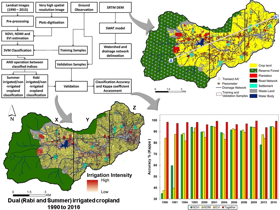
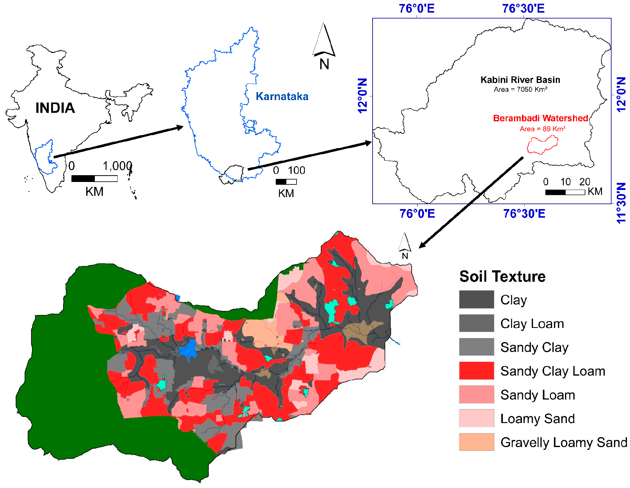
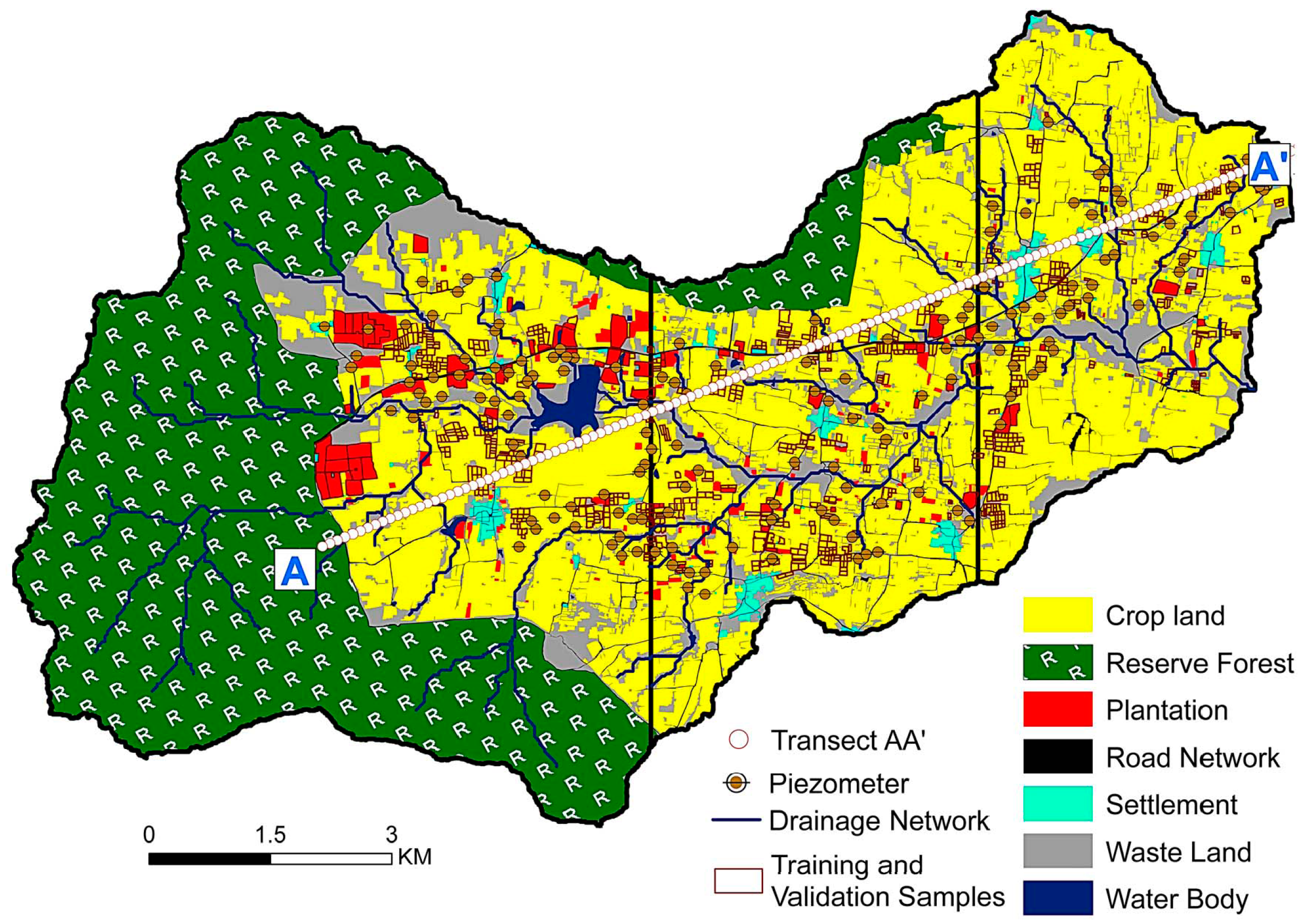
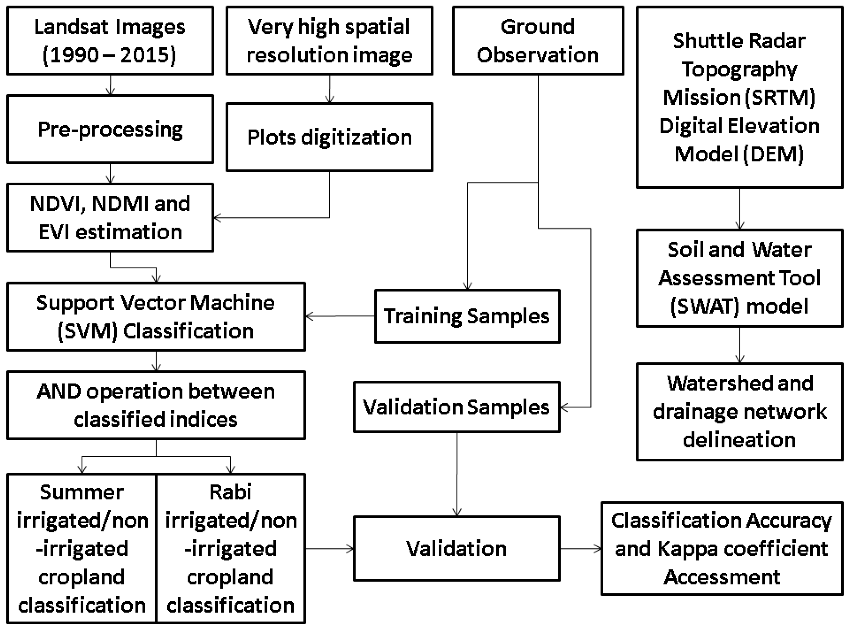
The objectives of this study were to assess the potential of optical indices derived from available cloud free multitemporal Landsat images for estimating the historical evolution of irrigated cropland area and to evaluate the impacts of this evolution on groundwater depletion in a semi-arid region of Southern India. For calibration, we used a large ground surveyed dataset of the Berambadi experimental watershed. The ground observations of irrigated and non-irrigated farm plots were done by surveying farmers’ fields from 1990 to 2016. It was noticed that the irrigated cropland classification requires time-series of vegetation indices [37,44,50]. Moreover, it has been shown that classification accuracy is higher when using multiple vegetation indices vs. 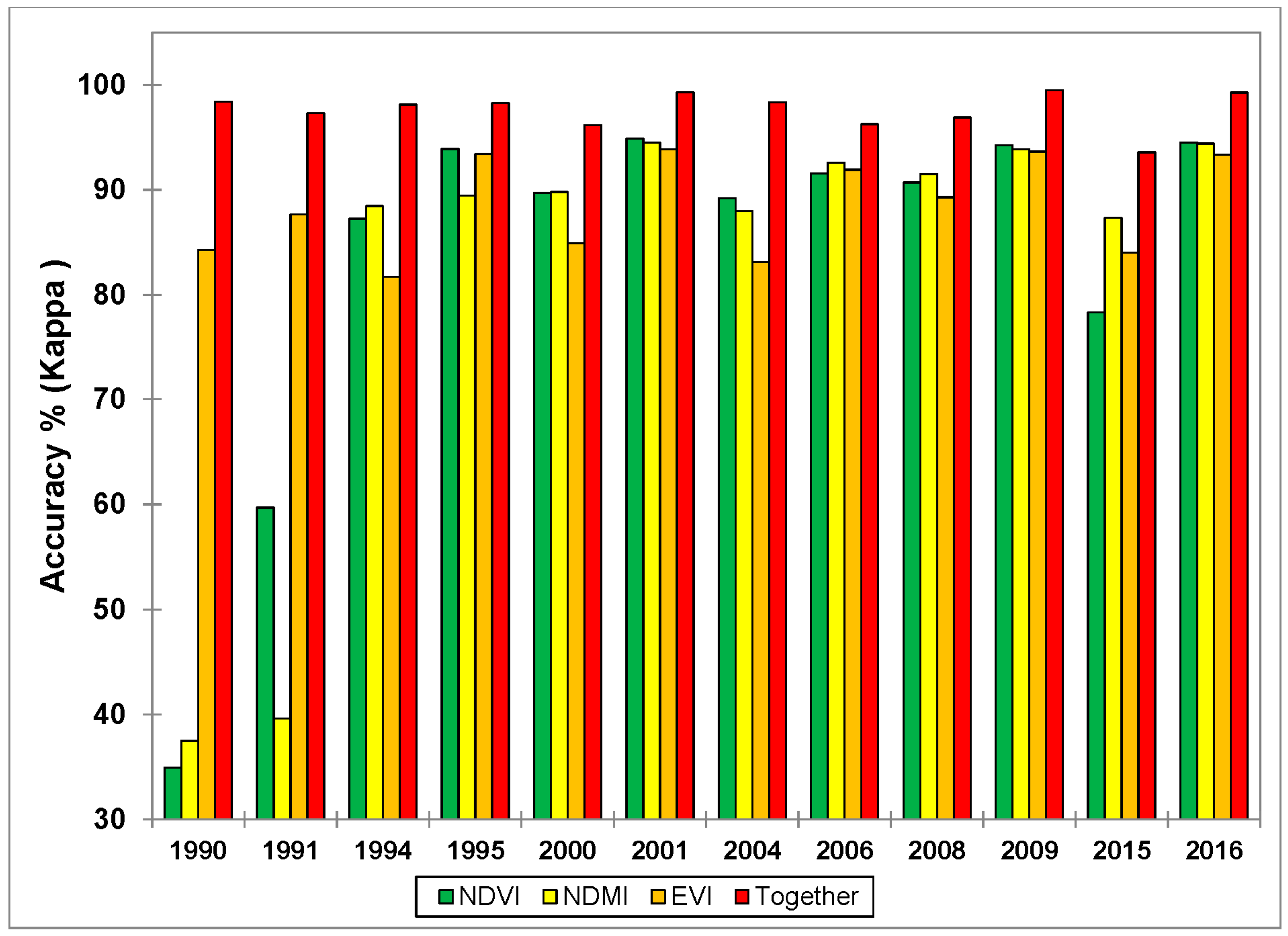single vegetation index in case of using one single date image [51]. One index was not able to consistently classify irrigated area using a single image, while in a combination of multiple indices high and consistent accuracy was observed. While applying this method to a watershed in India, we characterized the spatial heterogeneity in the dynamics of irrigation development across the watershed, and it links with the groundwater resource depletion.

2. Material and Methods

2.1. Study Area

The Berambadi watershed (89 km²) is located in the Gundlupet taluk, Chamrajanagara district of Karnataka in South India and belongs to the Kabini River basin which is a major tributary of the Cauvery River (Figure 1). The Kabini Critical Zone Observatory [52] has been monitored since 2002 by the Indo-French Cell for Water Science The Berambadi watershed has been developed as a calibration (CAL) and validation (VAL) site for various satellite mission like Radarsat2 [53], Soil Moisture and Ocean Salinity (SMOS) [53,54] and RISAT-1 under the project Assimilation of Multi-satellite at a Berambadi watershed for Hydrology And land Surface experiments(AMBHAS).

The soil type in the Berambadi watershed is categorized in seven major soils (Figure 1) at 1:50,000 scale by National Bureau of Soil Survey and Land Use Planning (NBSSLUP) [53]. Major LULC of the watershed is agriculture (approx. 52%), reserved forest (approx. 32%) and other minor classes include settlement, water bodies, wasteland, and road networks (Figure 2). A survey carried out in 2013 showed that the average farm size is 1.2 ha, 60% of the farmers have access to irrigation in at least a portion of their land, and selling or lending water between farmers is anecdotal [55]. Irrigation techniques cause soil salinization in croplands close to the watercourses [56]. Bedrock is granitic gneiss, and the aquifer is composed of a regolith layer of 15 m on average underlain by fissured and fractured rock layers [57]. This aquifer has a low transmissivity and typically one tube well cover less than 1 ha cropland for the irrigation [51]. Nevertheless, groundwater is virtually the only source of drinking water and irrigation. The number of tube wells has increased steadily during the last 15 years (minor irrigation census data from the ministry of water resources [30,58]).

Climate is tropical sub-humid with an annual rainfall of 800 mm and annual potential evapotranspiration of 1100 mm. The rainfall displays a strong inter-annual variability with decadal trends [19]. It is dominated by a monsoon regime, with the orographic effect of the Western Ghats generating a steep precipitation gradient along the West-East axis [59]. Based on the traditional cropping practices the main cropping seasons (

Table 1. Crop calendar of the experimental watershed.

	Summer Season	Kharif Season	Rabi Season
	Mid-Jan to Mid-May	Mid-May to Mid-Sept	Mid-Sept to Mid-Jan
Non-irrigated crops		Maize	Maize
		Country beans	Country beans
		Sunflower	Chickpea
		Marigold	Groundnut
		Sorghum
		Finger millet
Irrigated crops	Onion	Onion	Tomato
	Watermelon	Chilli	Solar beans
	Beetroot	Beetroot	Garlic
	Cabbage		Cabbage
	Tomato		Beetroot
		Turmeric (8 to 9 months)
	Sugarcane (12 months)
	Banana (12 months)

) are predominantly divided into three sections: Southwest monsoon or Kharif season (mid May to mid September) followed by Northeast monsoon or Rabi season (mid September to mid January) and the dry season or Summer season from mid January to mid May. Commonly farmers are following these cropping seasons for the cultivation with a time lag of one month, due to local weather condition or farmers strategy (i.e., economy, groundwater availability, and other personal planning). According to the Indian Meteorological Department (IMD) seasons in India are divided into four sections: winter season (January and February), pre-monsoon season (March to May), southwest monsoon season (June to September) and post-monsoon season (October to December).

During Kharif season, most of the agricultural area is cultivated, and a large diversity of crops are found, either rainfed or irrigated [60]. During Rabi season, the area under cultivation decreases with respect to the Kharif season and majority of crops are irrigated. Summer season cultivation is possible only with groundwater irrigation.

With the availability of groundwater irrigation, farmers usually tend to switch from traditional rainfed crops to water-intensive crops. As electricity for pumping is virtually free for farmers [11], crop choice depends mostly on groundwater availability and capacity to invest in inputs (seeds, fertilizers, pesticides, and labor). Irrigated crops with long crop cycles (e.g., turmeric, sugarcane, banana) are preferred when groundwater resource is abundant. The short cycle crops (e.g., onion, garlic, beetroot, cabbage) are used when the long-term availability of groundwater is not granted. In the valley region of the watershed, the majority of farmers switched from traditional rainfed crops to irrigated croplands. In some parts of the up-streams (upland areas), groundwater is used as a supplement during monsoon season for all crops.

Rabi cropping season is also known as post monsoon or second season. Rabi season is supported with groundwater irrigation resources. In the case of the poor Northeast monsoon, the majority of farmers are fully dependent on groundwater resources. Maize, horse-gram groundnut, and gram are the major rainfed crops in this season and beans, garlic, beetroot, sugarcane, and banana major irrigated crops (Table 1). However, maize can be found with or without irrigation in the watershed. In the case of non-sufficient precipitation, farmers are entirely dependent on the groundwater to cultivate their farmlands, as there is no other source of irrigation like a canal. The majority of farmers with borewell facility are priorities this season as the groundwater level arises after monsoon rainfall. Banana and Sugarcane are having a life cycle of 12 to 14 months, and both crops are initiating in the rabi season with 100% irrigation requirement. After monsoon season usually groundwater level rises and accordingly farmers plan for the irrigation in rabi (post-monsoon) season. In regions with low groundwater yield, farmers plan for non-irrigated crop or short duration cash crops, such as garlic or vegetable. However, with good groundwater yield farmers generally cultivates banana or sugarcane.

During summer season farmers are wholly dependent only on groundwater resources, as there is no other alternate source of irrigation in the watershed as the probability of rainfall occurrence is very low during the summer season. Farmers with sufficient groundwater yield are only cultivating crops in this season and all croplands in this season refer to 100% irrigated cropland. In summer season apart from extended rabi crops (like banana and sugarcane), farmers prefer to grow vegetables (like cabbage, beetroot, onion, tomato) and fruit (like watermelon) (Table 1). Crops cultivating in this season having high water demand.

2.2. Dataset Used in the Study

The irrigation history is developed using multi-temporal Landsat satellite images from the year 1990 to 2016. The study is focused on the post-monsoon (rabi) and summer (zaid) season, as the monsoon (kharif) season is mostly cloudy. The Shuttle Radar Topography Mission (SRTM) product 1 arc-second (30 m spatial resolution) Digital Elevation Model (DEM) was used for drainage and watershed delineation. Google Earth image, IRS (Indian Remote Sensing) LISS-IV (Linear Imaging Self scanning Sensor) and SPOT-6 (Satellite Pour l’Observation de la Terre) images were used for cropland parcel delineation.

2.2.1. Landsat Data

Multi-temporal Surface Reflectance (SR)-based products from Landsat (30 m spatial resolution) were used for irrigated vs. non-irrigated croplands classification. Twelve available cloud-free images (with approximately 5 year interval) were downloaded from the United States Geological Survey (USGS) website, includes ten Landsat 5 Thematic Mapper (TM) images and two Landsat 8 Optical Land Imager (OLI) images (

Table 2. List of the dataset used with Day Of Year (DOY), season and sensor specifications (Thematic Mapper (TM), and Optical Land Imager (OLI)). One image is considered per year for each cropping season.

Year	Rabi Season	Summer Season
	Date (DOY (Sensor))
1990–1991	26-12-1990 (360 (TM))	28-02-1991 (059 (TM))
1994–1995	05-12-1994 (339 (TM))	12-04-1995 (102 (TM))
2000–2001	21-12-2000 (356 (TM))	11-03-2001 (070 (TM))
2004–2006	16-12-2004 (351 (TM))	09-04-2006 (100 (TM))
2008–2009	27-12-2008 (362 (TM))	01-03-2009 (060 (TM))
2015–2016	31-12-2015 (365 (OLI))	20-12-2016 (080 (OLI))

). These twelve images span six agricultural years, with six rabi seasons and the following six summer seasons. Dates are towards the end of the respective seasons, corresponding to the stage of crop maturity. India being a tropical country cloud-free satellite images are rarely available during the Kharif cropping season. Therefore, while non-availability of images is the main limitation for using optical satellite images in monsoon regime contexts [18], the present study is restricted to the rabi and summer cropping seasons.

2.2.2. Agricultural Parcel Delineation

Accurate parcel delineation is essential to perform relevant classification with remotely sensed data, although it is challenging [61]. In the study area, this was challenging as available cadastral maps were established in the early XX century, and since then cadastral boundaries have often been divided into smaller fields belonging to different farmers. Currently, farmer’s landholding is about 1 ha on average [13]. Generally, farmers like to diversify land uses in order to reduce the risk of crop failure; they often divide larger fields into small-size parcels even when the same crop is cultivated in all of them, to allow a diversity of cultural practices. In fact, there is the tendency of farmers to merge or divide parcel across seasons or years. For classification, performing the analysis using the smallest parcel size minimizes the risk considering heterogeneous units. Hence we first delineated all individual parcels that could be identified using the 2 m spatial resolution google earth image of the year 2012, which was the best available resolution. Then all parcels were re-examined using successively 2013, 2014 and 2015 LISS IV (5 m spatial resolution) and 2016 SPOT-6 (1.5 m spatial resolution) satellite images and when a parcel division was identified, corresponding plots were delineated.

2.2.3. Ground Observation

The ground observation was divided into two parts: manual groundwater level data collection in various cropping seasons and irrigated/non-irrigated cropland survey with farmers.

The intensive irrigated and non-irrigated cropland ground observation survey was conducted with the help of local farmers (Figure 2). The complete survey was done with individual interviews of around 80 to 120 farmers. Extensive field visit was undertaken to cover all land parcels in collecting the irrigation history in the watershed. To maintain the survey accuracy, the information collected was cross-checked with the adjacent farmers. The questions include: “When was the borewell installed and/or re-installed?”, “How deep is the borewell?”, “What are the pump specifications?”, “Which crop were growing during the study period?”, “What is the groundwater yield?”, What are the borewell re-drilling and service history?”, “How much cropland area is cultivated using borewells?”, “Are they happy with groundwater yield?”, “Did they switch from traditional crops to other crop types?” etc. While doing ground survey with farmers help, we noticed that in 90′s the plot size was bigger than present in present (year 2016). Farmers divided the irrigated cropland according to their financial resources and groundwater availability. As shown in

Table 3. Training and validation samples of irrigated and non-irrigated cropland in the Berambadi watershed.

Year	Irrigated	Non-Irrigated	Total
2015–2016	76	204	280
2008–2009	72	380	452
2004–2006	69	412	481
2000–2001	77	374	451
1994–1995	85	352	437
1990–1991	48	342	390

, around 2500 parcels were used as samples for supervised classification using SVM algorithm. For the calibration of SVM model, 50% random and spatially distributed parcels were selected and remaining 50% random parcels were used for validation [62,63]. Care was taken to perform precise ground surveys and farmer interviews to obtain precise information on cropping and water management practices.

2.2.4. Groundwater Level Monitoring

The groundwater level and borewell yield in the Berambadi watershed are monitored by spatially distributed 205 operational piezometers (Figure 2). Most of these piezometers belong to the farmers, who are using them for the irrigation purposes. Monthly groundwater level monitoring is realized since May 2010 during non-pumping hours. The transect AA’ is drawn to retrieve the groundwater level from upstream to downstream of the watershed. Inverse Distance Weighting interpolation was done at the watershed scale using distributed piezometers for three cropping seasons. Along the transect AA’ the interpolated groundwater level was extracted for various cropping seasons with 100 m interval.

2.3. Image Pre-Processing for Irrigated and Non-Irrigated Cropland Classification

Landsat Multitemporal Images Calibration and Indices Estimation

All pre-processed (geo-referencing, atmospheric correction, optical indices estimation) Landsat images and indices (NDVI, NDMI and EVI) were downloaded from ESPA (Earth Resources Observation and Science (EROS) center Science Processing Architecture) project of USGS [64]. The atmospheric correction was performed using the Landsat Ecosystem Disturbance Adaptive Processing System (LEDAPS) algorithm [64]. The surface reflectance and atmospheric correction were performed using Second Simulation of a Satellite Signal in the Solar Spectrum (6S) radiative transfer model [64,65]. LEDAPS is a highly standardized and stable automatic surface reflectance modeler, which can ensure comparability of reflectance from sensors of Landsat satellites [21,51,64,66]. Due to the cloud cover and sensor malfunctioning, the temporal resolution cannot maintain the same [21]. The pre-processed NDVI, NDMI and EVI optical indices were estimated using equations mentioned in

Table 4. Indices used were: Normalized Difference Vegetation Index (NDVI), Normalized Difference Moisture Index (NDMI) and Enhanced Vegetation Index (EVI). Where G = 2.5 (the gain factor), ρ is the atmospherically corrected value for near-infrared (NIR), Red and Blue bands, C1 and C2 are coefficients with constant values 6.0 and 7.5 respectively, and L is the soil adjustment factor, and its value is 1.0 [67].

Indices Name	Equation
NDVI	$\mathrm{NDVI}=\frac{\mathsf{\rho }\mathrm{NIR}-\mathsf{\rho }\mathrm{Red}}{\mathsf{\rho }\mathrm{NIR}+\mathsf{\rho }\mathrm{Red}}$
EVI	$\mathrm{EVI}=\mathrm{G}\frac{\mathsf{\rho }\mathrm{NIR}-\mathsf{\rho }\mathrm{Red}}{\mathsf{\rho }\mathrm{NIR}+\mathrm{C}1\left(\mathsf{\rho }\mathrm{Red}\right)-\mathrm{C}2\left(\mathsf{\rho }\mathrm{Blue}\right)+\mathrm{L}}$
NDMI	$\mathrm{NDMI}=\frac{\mathsf{\rho }\mathrm{NIR}-\mathsf{\rho }\mathrm{SWIR}}{\mathsf{\rho }\mathrm{NIR}+\mathsf{\rho }\mathrm{SWIR}}$

[64]. All optical indices were resampled using nearest neighbor (NN) resampling method to the pixel size 5 m spatial resolution for a better precise mean and standard deviation at agriculture plot scale [33].

2.4. Data Processing

The overview of the comprehensive methodology to classify multi-temporal irrigated and non-irrigated cropland area is presented in Figure 3.

The parcel scale median value [53] and standard deviation (SD) were estimated for the various indices (NDVI, NDMI, and EVI). Parcel mean values were estimated for all 36 optical indices (3 indices × 12 multi-temporal products).

2.4.1. Support Vector Machine Classification

The Support vector machine classification was performed using the scikit-learn library [45]. Support vector machine classification was done individually for the various optical indices (NDVI, NDMI, and EVI) using 50% random spatially distributed intensive ground observed training samples. Remaining 50% random samples were used for the classification validation. The comprehensive methodology leads to identify irrigated and non-irrigated croplands.

2.4.2. Irrigated Cropland Mapping

To remove the classification overshoot, it was noticed that the indices together could perform better than the individual one. Therefore, the decision rule in the form of AND boolean operator was implemented on SVM classified outputs of these indices, and we have found that it removed overshoot error of irrigated cropland outputs.

After generation of all irrigated cropland maps, the kappa coefficient was estimated. Kappa index is considered to be a better index for determining classification accuracy from the confusion matrices [34,68]. The primary results of irrigated and non-irrigated croplands were generated, and the kappa coefficient was calculated for all classified outputs. These individually classified outputs were further used to estimate irrigation history and to identify the evolution of dual season irrigated cropland (post-monsoon and summer cropping seasons) in the watershed. The validation of classified cropland parcels was done with randomly selected 50% (around 1250 plots) of ground observed datasets.

2.4.3. Irrigation Intensity Mapping

After assigning 1 and 0 to respectively irrigated and non-irrigated croplands, the multitemporal values obtained for each plot were summed to produce the irrigation intensity maps. The irrigation intensity maps were generated for the post-monsoon and summer cropping season by adding multitemporal images of concern seasons. The cumulative irrigation intensity map for the year 1990 to 2016 was generated by adding all 12 images, including both cropping seasons. This process gives a synoptic view of the spatial distribution of irrigated cropland intensity in the watershed.

3. Results and Discussion

The first subsection explains about plot (parcels) delineation procedure and plot size variation in the watershed. The second subsection shows inter-comparison of results obtained from different indices for rabi and summer seasons. The third subsection is about spatiotemporal irrigated cropland evolution in the berambadi watershed. The impact of intensive irrigation on groundwater is discussed in the fourth subsection.

3.1. Plot Delineation

Approximately 19,600 parcels were digitalized in the Berambadi watershed out of which 18,500 parcels were identified as agricultural land. Except for very few parcels of more than 2 ha, which were identified as plantations, the other parcels were extremely small, with a mean of 0.2 ha (Figure 4). Classifying satellite images, in this case, is challenging to analyze the progression of groundwater irrigation over time.

3.2. Irrigated and Non-Irrigated Cropland Classifications

The kappa accuracy (%) of irrigated and non-irrigated cropland classification using NDVI, NDMI, and EVI, individually and together multitemporal images (36 images (12 dates × 3 indices)) of rabi and summer cropping seasons is shown in Figure 5.

The classification was performed with SVM algorithm using EVI, NDMI, and NDVI indices. First, SVM algorithm was applied separately to each date and then to the rabi season dates and the summer season dates considered as two different datasets, and finally to all dates considered together as one dataset. It was evident in Figure 5 that, individually all three indices (EVI, NDVI, and NDMI) were given poor classification outputs when compared the same with combined indices. For the year 1990–1991, the classification results of each of the NDVI and NDMI were poor than EVI, even though combined indices performed further better than EVI. From 1994 to 2016 all indices improved the irrigated cropland classification performance with an error of 15 to 20%. However, indices performed higher classification accuracy together than the individual. Besides, these results confirm that SVM performs very well for the classification of irrigated cropland [37,46].

3.3. Irrigated and Non-Irrigated Cropland Analysis during Rabi Season (Post-Monsoon)

3.3.1. Irrigated and Non-Irrigated Cropland Evolution

The spatial distribution of irrigated and non-irrigated (or fallow land) cropland areas for the rabi cropping season depicted in Figure 6 with the approximately five-year interval from the year 1990 to 2015. It was noticed that in the 1990s few farmers (approximately 5%) with irrigation facility was cultivating in rabi season. In 1994, about 16% irrigated cropland clustering was identified in the downstream of the watershed. The results show that the farmers were interested to grow irrigation crops in rabi season. As shown in

Table 5. Rabi season irrigated cropland evolution from 1990 to 2015.

Year	Total Number of Parcels	Total Area (ha)	Irrigated Cropland Area (%) with Respect to the Total Agricultural Cropland
			Upstream (X)	Middle Stream (Y)	Downstream (Z)	Total
1990	812	201.4	3.45	5.92	4.16	4.57
1994	2431	684.24	16.18	16.00	14.36	15.54
2000	3123	859.73	17.78	22.47	18.14	19.52
2004	2346	649.29	14.59	14.48	15.19	14.74
2008	3584	936.31	24.39	18.46	21.19	21.26
2015	4934	1380.36	51.13	24.15	18.81	31.34

, during the year 2015 rabi season irrigated cropland has reached 31%, compared to 21% in the year 2008, which requires a huge quantity of groundwater for the crop irrigation. The rabi season irrigated area in the up and middle stream regions has increased 27% and 6%, respectively during 2008 to 2015 (Table 5). However, in the downstream, the irrigated area has been reduced by 2.5% for the same period. These figures indicate farmers’ interest for rabi season irrigation in the upstream region.

3.3.2. Irrigated and Non-Irrigated Cropland Spatial Evolution

The total irrigated cropland area was divided into the three zones upstream, middle stream and in downstream. The temporal variation of irrigated cropland was analyzed for the rabi season in these zones (regions). The regional irrigated cropland statistics gave an idea about their shifting towards upstream. The irrigated cropland in the upstream has significantly increased during last decade (Figure 7). However, due to tremendous depletion of groundwater in the downstream, the total rabi season irrigated cropland area of downstream got stabilized.

3.3.3. Irrigated and Non-Irrigated Cropland Intensity

The combined spatiotemporal map of the irrigated area was generated to distinguish the spatial distribution of high and less intensity irrigation practices. The light red to dark red color in the map shows the temporal intensity of irrigation (Figure 8). The irrigated croplands are clustered to the drainages and shifting towards upstream of the watershed. Shallow groundwater level in the upstream is attracting farmers to adapt irrigation practices during multiple cropping seasons. The irrigation intensity map (Figure 8) shows that new rabi irrigating cropland are emerging in the upstream. This tendency of farmers to adopt irrigation led them to pump an enormous amount of groundwater to fulfill the crop water requirement. This intensive irrigation activity can further deplete upstream groundwater, which can disconnect the baseflow and can disturb adjacent reserve forest ecology.

3.4. Irrigated and Non-Irrigated Cropland Analysis during the Summer Season

3.4.1. Irrigated and Non-Irrigated Cropland Evolution

Historical evolution of irrigated and non-irrigated cropland maps for summer cropping season (Figure 9) is also providing insightful information on spatial distribution and evolution of irrigation in the watershed. The detailed maps confirmed the observation that irrigation was preferentially developed along the valleys. Due to the insufficiency of high-resolution satellite images, a good number of studies used coarse resolution satellite images for the cropland classification with high definition gaps in rainfed and irrigated croplands [39].

In 1991, few farmers with irrigation facility were growing summer crops. These farmlands existed for the most part near the outlet of the watershed. Slowly with time summer irrigated croplands moved towards upstream (Figure 9), but they were clustered around mainstream of the watershed. Summer irrigated cropland expansion in the watershed was noticed from 1991 to 2016 (Figure 10). Due to intensive irrigation impact on groundwater farmers started quitting taking the risk of crop failure in the case of poor borewell yield [52]. In 2016 most of the downstream farmers stopped summer irrigation, as groundwater depleted drastically. It is evident in Figure 9 that at present mostly summer irrigated cropland clusters exist in the upstream area of the watershed along the drainage. The total summer season irrigated area was increased threefold from 1991 to 1994, and after that, it got stabilize till 2009, and then it reduced to 2.5% in 2016 (

Table 6. Summer season irrigated cropland evolution from 1991 to 2016.

Year	Total Number of Parcels	Total Area (ha)	Irrigated Cropland Area (%) with Respect to the Total Agricultural Cropland
			Upstream (X)	Middle Stream (Y)	Downstream (Z)	Total
1991	816	210.55	2.74	4.76	6.92	4.78
1995	2406	694	19.82	13.31	14.52	15.76
2001	2560	684.4	14.24	16.39	16.06	15.54
2006	2837	789.64	21.69	16.66	15.65	17.93
2009	2805	723.79	16.79	15.48	17.23	16.43
2016	2170	616.24	19.06	13.60	9.28	13.99

).

3.4.2. Irrigated and Non-Irrigated Cropland Spatial Evolution

Summer cropping is entirely dependent on the irrigation, and in the Berambadi watershed, there is no alternate source for the farmers except groundwater irrigation. Irrigated area has increased tremendously during 1991–1995 (Figure 10). From 1995 the upstream part of the watershed was leading in total irrigated cropland area as compared to downstream (Figure 10). Due to intensive groundwater and a huge number of borewells in the downstream, the farmers belong to the downstream region of watershed started quitting to grow summer season crops.

3.4.3. Irrigated and Non-Irrigated Cropland Intensity

Summer season cropping is wholly dependent on the groundwater resources in the watershed. In 90′s the irrigated cropland was mainly at downstream and slowly it clustered around all three main tanks of the watershed; however, presently all tanks are dried. The spatiotemporal map was generated from low intensity (once irrigated) to high intensity (always irrigated) (Figure 11). The non-irrigated croplands (rainfed croplands) are shown in yellow color. These croplands were not under any irrigation in summer cropping season during the year 1990–2016. In the absence of rainfall and no surface water availability during summer cropping season, farmers generally irrigate the crops using groundwater.

3.5. Dual Season (Rabi and Summer) Irrigated and Non-Irrigated Cropland Analysis

3.5.1. Irrigated and Non-Irrigated Cropland Evolution

The total number of parcels of dual irrigated croplands has increased from 1990 to 2009, but during 2015–2016 the dual irrigated parcels have reduced (

Table 7. Dual irrigated cropland evolution from 1990 to 2016.

Year	Total Number of Parcels	Total Area (ha)	Irrigated Cropland Area (%) with Respect to the Total Agricultural Cropland
			Upstream (X)	Middle Stream (Y)	Downstream (Z)	Total
1990–1991	332	98.52	1.28	2.98	2.36	2.24
1994–1995	1072	356.4	11.34	6.51	6.60	8.09
2000–2001	1219	395.37	10.32	9.20	7.50	8.98
2004–2006	1028	345.26	10.41	6.75	6.50	7.84
2008–2009	1463	429.97	12.22	8.12	9.17	9.76
2015–2016	888	342.04	14.01	6.32	2.98	7.77

). At present farmers like to grow cash crops like turmeric, sugarcane, banana, onion, garlic, vegetables. All of these cash crops need intensive irrigation facility. Farmers with sufficient irrigation facility are switching to 2 or 3 irrigated crops per year. Apart from monsoon season, these farmers are cultivating crops in rabi and summer seasons. The total area is under dual irrigation, which is about 10% of total agricultural cropland (Table 7). These farmers have sufficient groundwater yield throughout the year for cultivation. These croplands are contributing maximum to the water loss in the watershed.

3.5.2. Irrigated and Non-Irrigated Cropland Spatial Evolution

The temporal evolution of dual irrigated cropland in upper stream, middle stream and downstream of the watershed is depicted in Figure 12. During 1994–1995 the dual irrigated cropland shoot-up in the upstream with an approximate 11% area occupation with respect to total cropland area of the upstream region. The high probability of groundwater yield in the upstream motivates farmers for dual season irrigation. As the groundwater of upstream region of the watershed is recharged by the adjacent humid reserve forest, this region helps to maintain dual irrigated cropland area from 1994–1995 to 2015–2016 (Figure 12). Middle stream and the downstream regions of the watershed has increased and stabilized their total irrigated cropland between 1994–1995 and 2008–2009. Intensive irrigation in the whole watershed depleted the groundwater by more than 50 m in downstream resulting the dual season irrigation depletion during 2015–2016. Due to over-exploitation of groundwater, many borewells were dried up and farmers lost their crops in last decade. After understanding the groundwater depletion pattern and poor borewell yield majority of farmers quit their plan for the summer crops in the downstream areas.

3.5.3. Irrigated and Non-Irrigated Cropland Intensity

Figure 13 shows the spatial distribution of dual cropping season intensity from 1990 to 2016. In 90′s the berambadi watershed had three major water bodies in downstream near the outlet of the watershed, one at middle stream and one at upstream (Figure 13). In 2017, the most significant perennial water body, which exists in the upstream of the watershed, also disappeared. Due to a continuous increase in irrigated cropland in the upstream, the farmers are exhausting their resources. In 1990s the groundwater yield in the upstream was better and surface flow also existed in monsoon and post-monsoon seasons. Economically strong farmers purchased big-sized farmlands (Figure 13) and started growing high water demanding crops like banana, sugarcane, coconut, turmeric, and vegetables. However, now these big farmers, as well as farmers in the middle stream and downstream, are dividing their croplands into smaller parcels for precision management and avoiding crop failure.

Figure 13 represents dual (rabi and summer seasons) irrigation croplands evolution in the watershed. Other than cultivating in summer and rabi seasons, these farmers are also cultivating in the kharif season. Intensive cropping of three seasons in a year is leading to extensive utilization of water resources, and use of various fertilizers is exerting significant negative impacts on the soil quality and groundwater availability [3]. The major dual irrigated croplands are clustered along the drainages or valleys of the watershed (Figure 13).

3.6. Impact of Intensive Irrigation on Groundwater

As per the Census of India 2011, the area under irrigation in the Gundulupet taluk is 27% of the net sown area with borewell density of 11 borewells/km². It was observed that the valley portions are having deeper groundwater levels, while in the topographically higher zones have relatively shallow groundwater level (Figure 14). This pattern of groundwater base flow is non-classical in hydrogeology. The Figure 14 also shows that borewell density in the valleys, and now the borewell failure rate is also increased significantly in the valleys of the watershed.

Farmers in the watershed rather than depending on rainfall they tend to use groundwater extensively. During last three decades, the most of the farmers switch from rainfed to irrigated cropping. The number of borewells in the watershed are growing unceasingly from 90′s [52]. A total of 13 villages exist in the watershed, and we have found the number of borewells is on the rise. During weak monsoon, farmers keep borewell option open as an alternative [52]. Figure 14 highlights large change in groundwater levels due to rapid addition of borewells. Downstream groundwater depleted by 40 to 50 m due to intensive irrigation history and drainages runs dry. Now irrigated cropland clustered in the valleys and shifted towards upstream of the watershed. This uncontrolled growth in several borewells can cause further groundwater depletion in the upstream region of the watershed and will have a severe impact on the adjacent reserve forest groundwater level located in the upstream area.

To understand the seasonal spatial variability of groundwater level in the watershed, we have interpolated the observed groundwater level dataset at watershed scale [3]. The transect AA’ shown in Figure 2 used to extract the groundwater levels with 100 m intervals for all three cropping seasons (kharif, rabi, and summer). The extracted interpolated groundwater level was plotted in Figure 14, with a total number of groundwater pumping borewells in villages, passes through the transect AA’. It is observed that the valleys are having a maximum number of borewells, as there is more probability to get good borewell yield.

The groundwater recharging in the monsoon (Kharif) cropping season and the groundwater level is at its highest level in a post-monsoon (rabi) season (Figure 14). This increased groundwater level tempts the farmers to plant banana and sugarcane in rabi season. In the summer season, groundwater irrigation continues with high evapotranspiration rate, which depletes groundwater at maximum level. Majority of summer irrigated cropland situated in the valleys of the watershed and neighborhood of water tank area. This overexploitation of groundwater and occupying the valleys for the cropping obstructs the surface flow. At present, there is no surface flow in the berambadi watershed, and all water bodies are completely dried, it happens first time in history after the construction of the berambadi water tank. This intensive irrigation is disconnecting the base flow [3] and depleting groundwater table in the valleys. This overexploitation of groundwater is affecting the ecosystem and creating various environmental issues.

4. Conclusions

Characterizing the spatiotemporal evolution of irrigated croplands is essential for sustainable resource exploitation in intensive agriculture areas. This study showed that available multitemporal remote sense data could be used to retrieve historical evolution of irrigation and its impact on groundwater resources. While we used Landsat multi-temporal imagery, it would be interesting in future studies to apply our approach on Sentinel 2 time-series to compare the results obtained with these two different types of datasets.

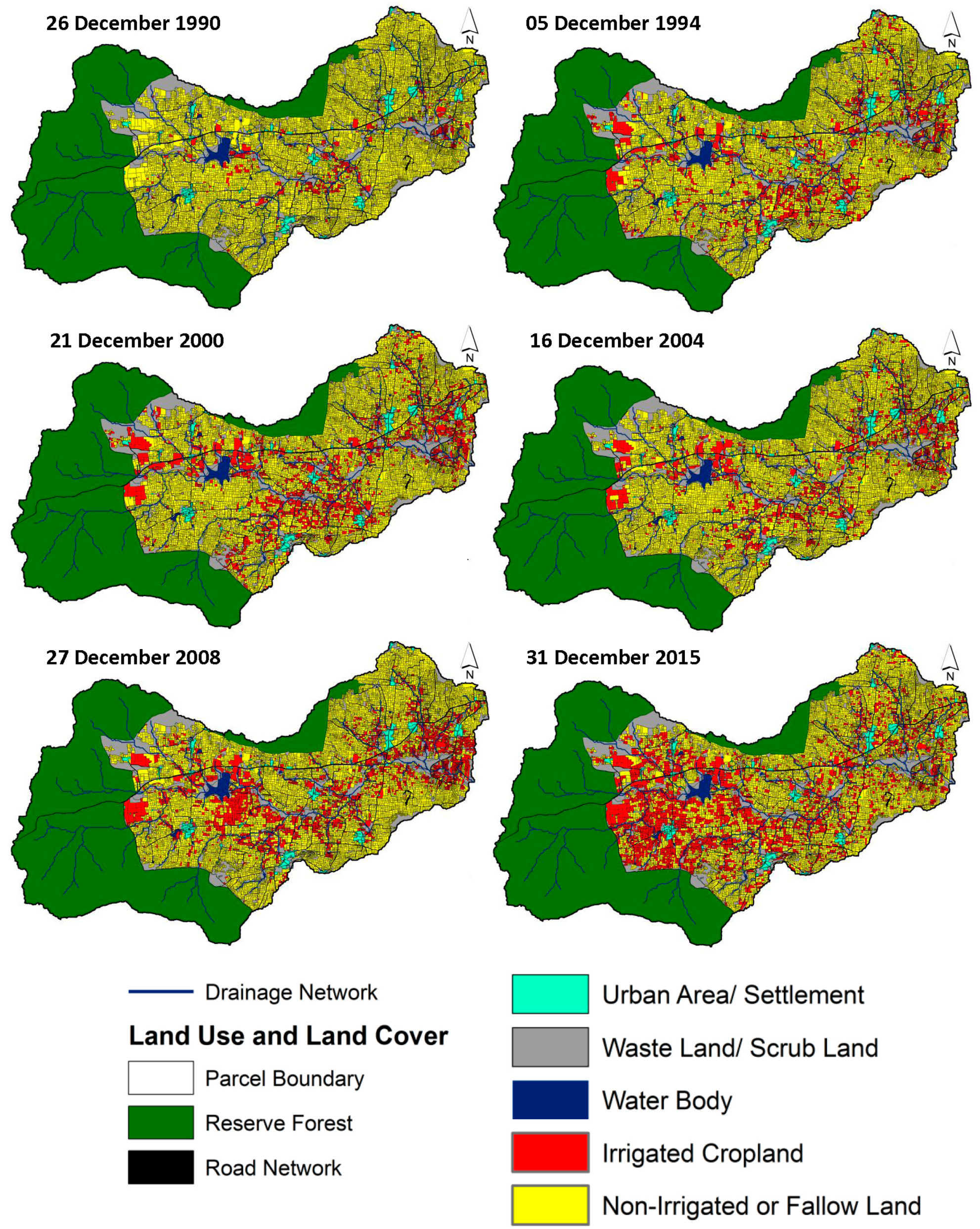
We have showed that the combined use of multispectral indices like NDVI (vegetation), EVI (soil impact correction to vegetation) and NDMI (moisture) could provide accurate classification of irrigated cropland. Using SVM algorithm (trained with intensive ground sample dataset) allowed us to generate irrigated cropland statistics for the past four decades in a semi-arid watershed in South India, which was a challenge considering with the small plot dimensions (less than 0.5 ha). The resulting irrigated and non-irrigated cropland classified maps were generated for rabi and summer seasons with high classification accuracy and kappa coefficient.

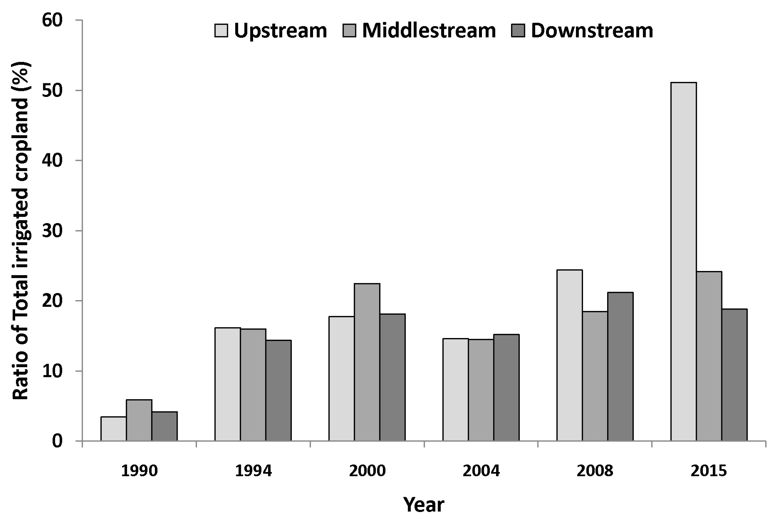
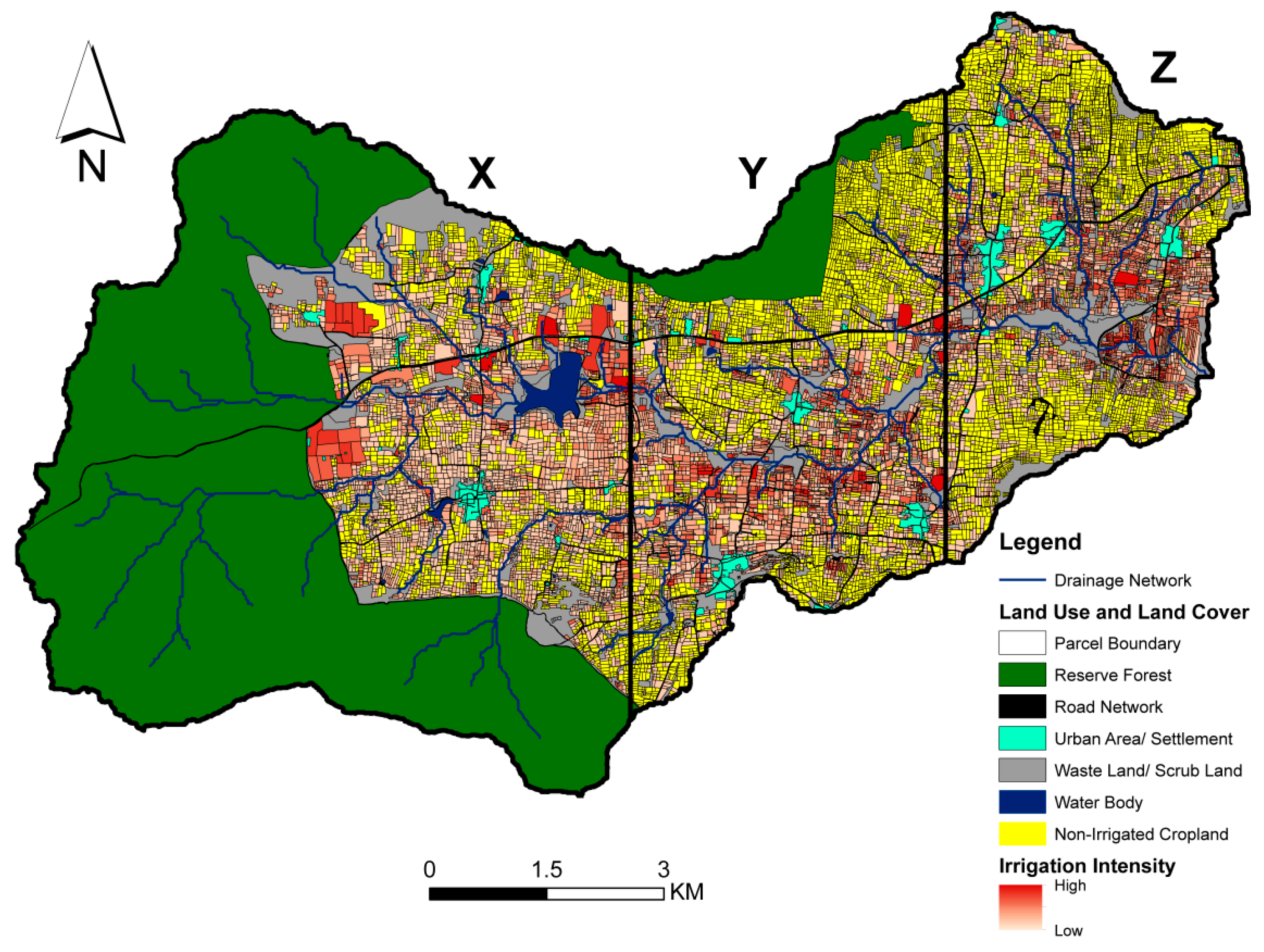
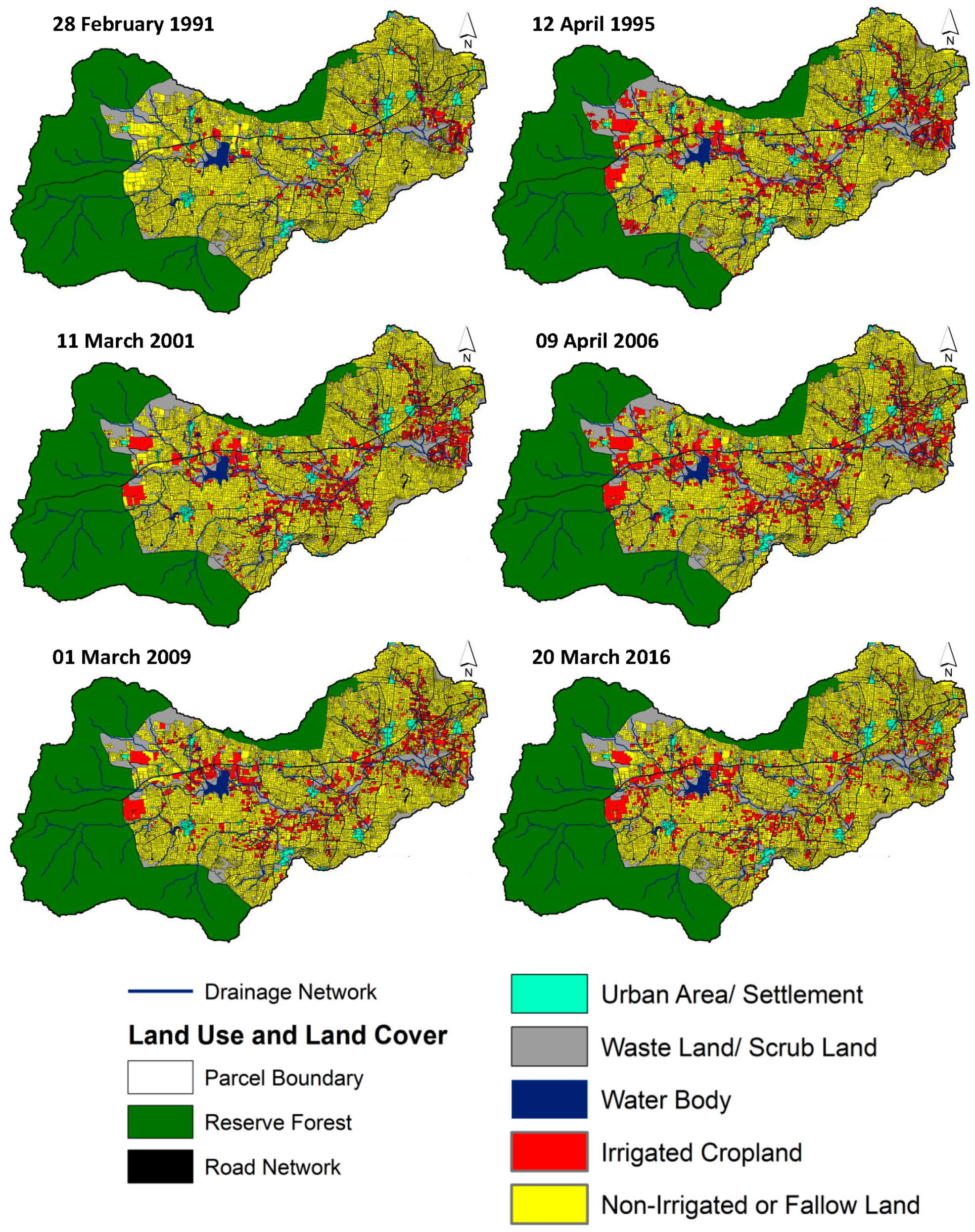
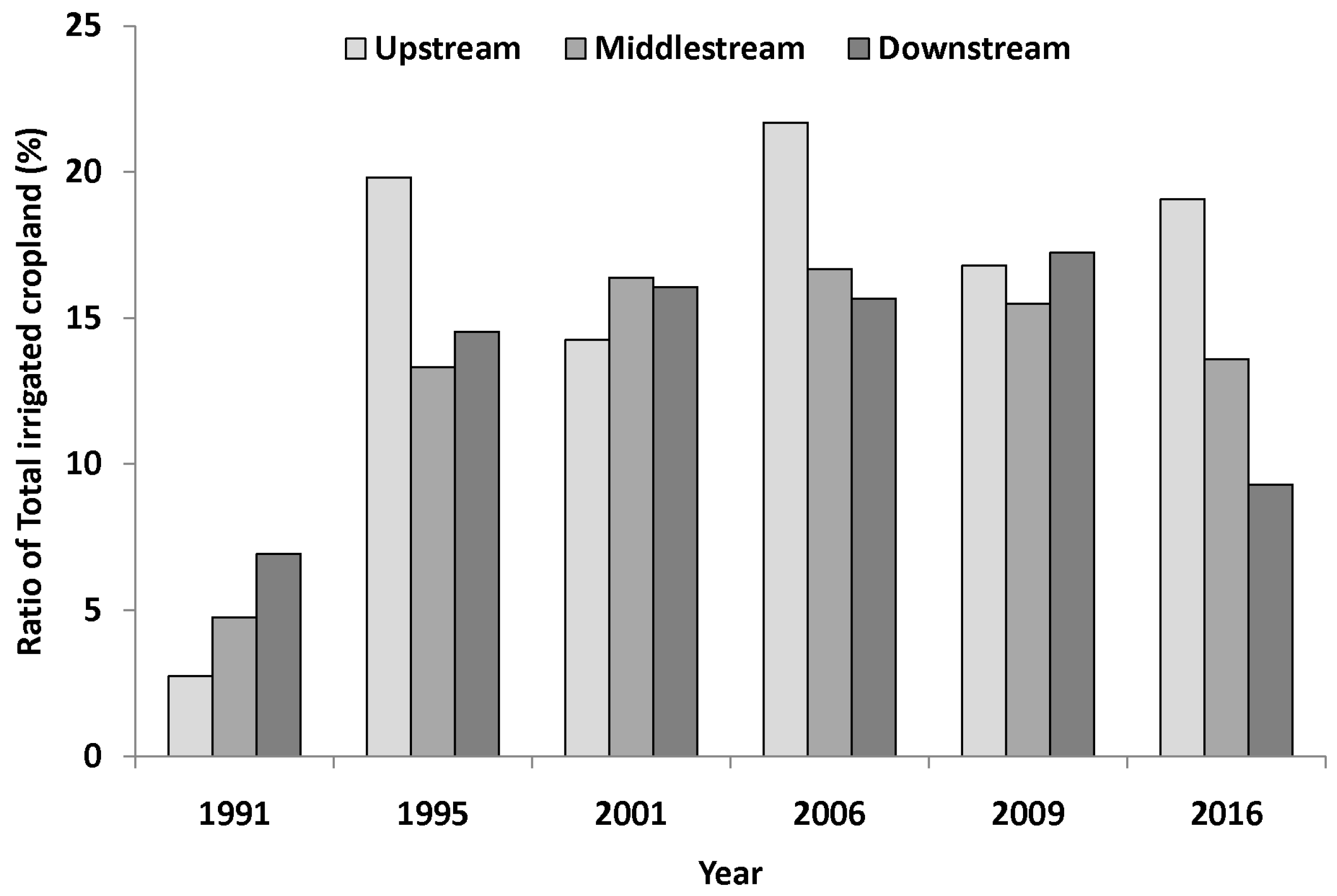
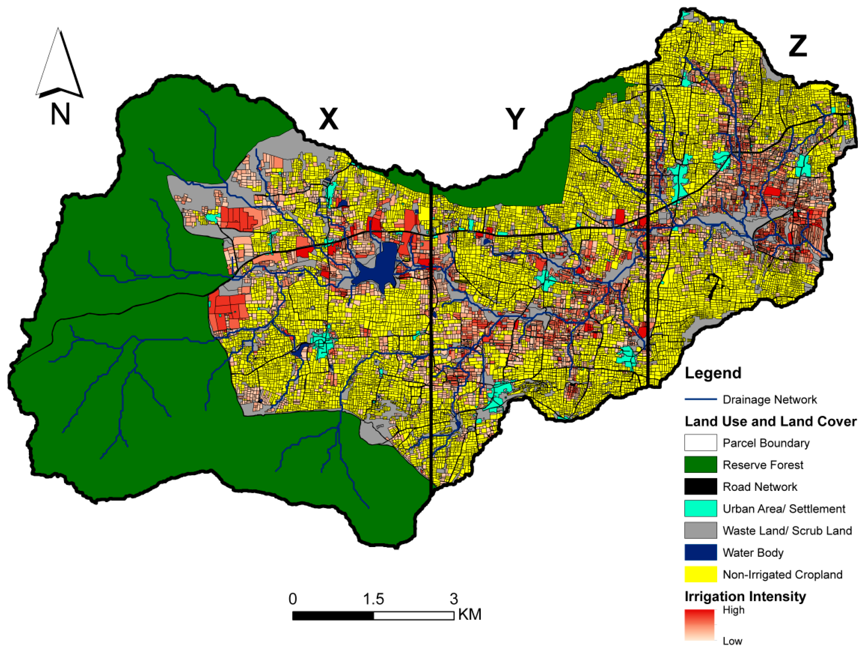
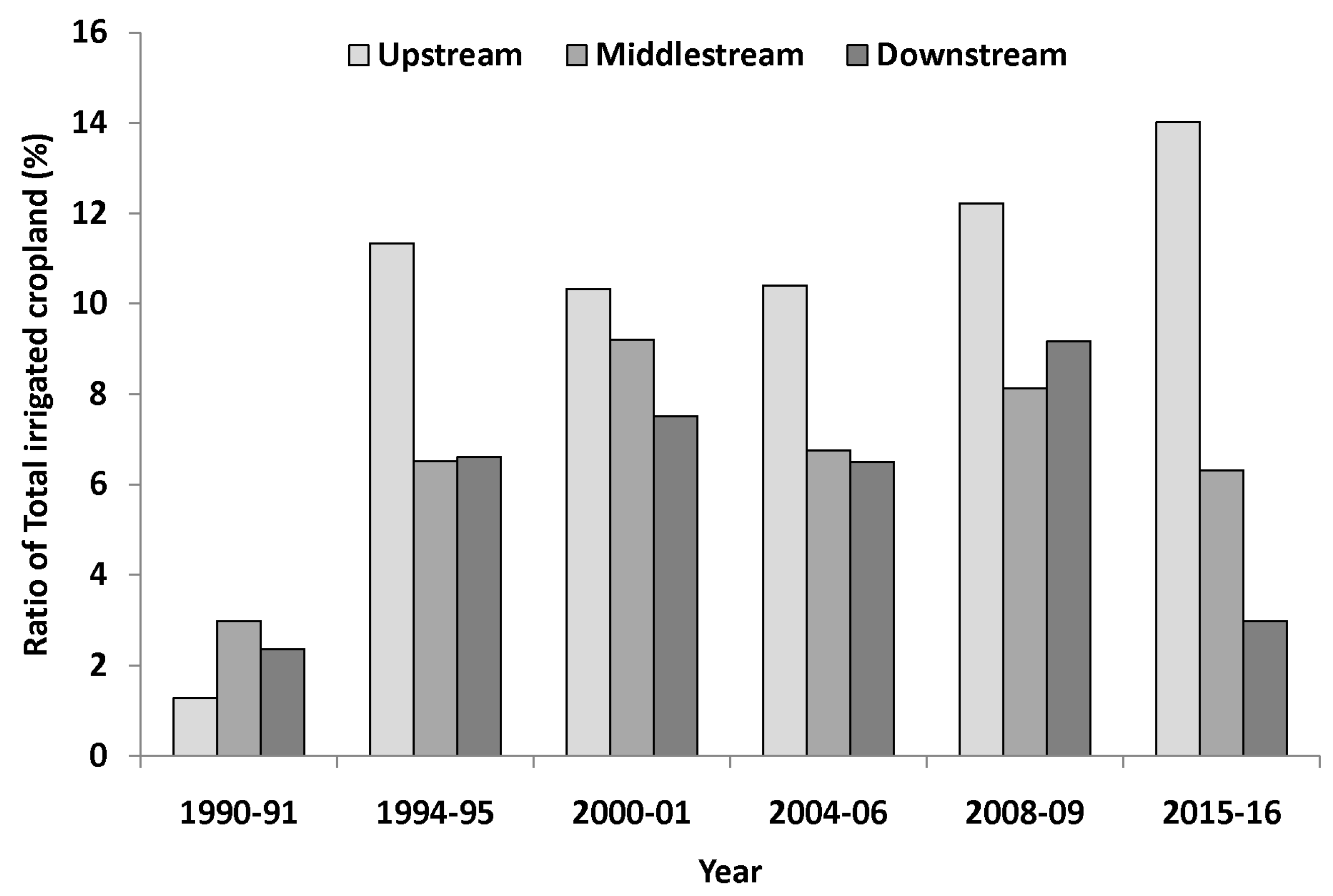
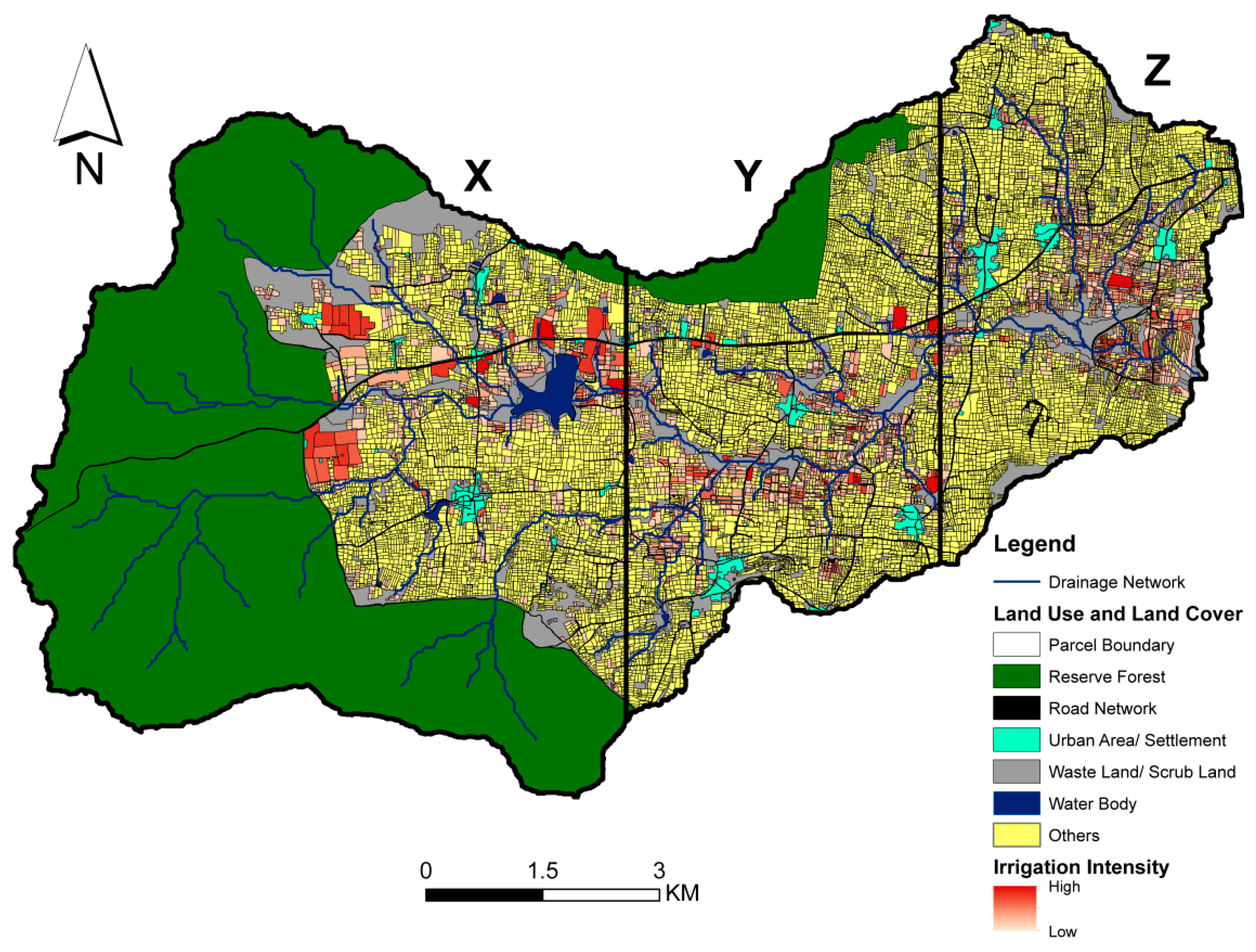
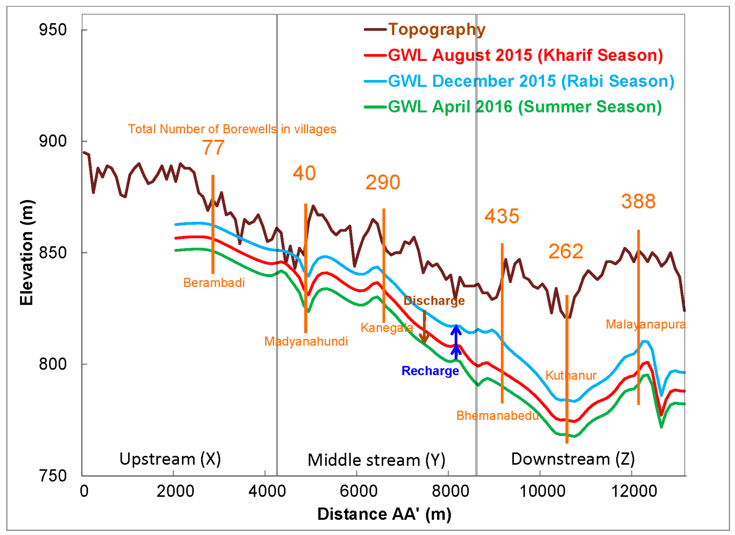
Results show the contrasted spatial distribution of irrigated cropland in the watershed and its evolution over time: while irrigation was developed very early in the valley areas in the East (downstream), it expanded recently to all the upstream areas while decreasing in the East. This was found consistent with the observed evolution of groundwater resources in the watershed: while in the East part groundwater was severely depleted since 2010, the decline in water table levels is more recent in the West.

The constructed irrigated cropland statistics can be used as an input to groundwater models for understanding the interactions between climate, agricultural practices, and water resources. They are also relevant to implement management strategies and support to policy making. Creating awareness among the farmers to adopt sustainable agriculture practices would perhaps the only way to escape from the onslaught of slow ecological disaster.

References

1. Shah, T. Climate change and groundwater: India’ s opportunities for mitigation and adaptation. Environ. Res. Lett. 2009, 4, 1–13. [Google Scholar] [CrossRef]
2. Fishman, R.M.; Siegfried, T.; Raj, P.; Modi, V.; Lall, U. Over-extraction from shallow bedrock versus deep alluvial aquifers: Reliability versus sustainability considerations for India’s groundwater irrigation. Water Resour. Res. 2011, 47, 1–15. [Google Scholar] [CrossRef]
3. Buvaneshwari, S.; Riotte, J.; Sekhar, M.; Kumar, M.S.M.; Kumar, A.; Louis, J.; Audry, S.; Giriraja, P.R.; Praveenkumarreddy, Y.; Moger, H.; et al. Science of the Total Environment Groundwater resource vulnerability and spatial variability of nitrate contamination: Insights from high density tubewell monitoring in a hard rock aquifer. Sci. Total Environ. 2016. [Google Scholar] [CrossRef]
4. Agarwal, A.; Marian, S.; delos Angeles, R.B.; Chéret, I.; Davila-Poblete, S.; Falkenmark, M.; Villarreal, F.G.; Jønch-Clausen, T.; Kadi, M.A.; Kindler, J.; et al. Integrated Water Resources Management; Global Water Partnership: Stockholm, Sweden, 2000; ISBN 9163092298. [Google Scholar]
5. Velpuri, N.M.M.; Thenkabail, P.S.S.; Gumma, M.K.K.; Biradar, C.; Dheeravath, V.; Noojipady, P.; Yuanjie, L. Influence of Resolution in Irrigated Area Mapping and Area Estimation. Photogramm. Eng. Remote Sens. 2009, 75, 1383–1395. [Google Scholar] [CrossRef]
6. Thenkabail, P.S.; Dheeravath, V.; Biradar, C.M.; Gangalakunta, O.R.P.; Noojipady, P.; Gurappa, C.; Velpuri, M.; Gumma, M.; Li, Y. Irrigated area maps and statistics of India using remote sensing and national statistics. Remote Sens. 2009, 1, 50–67. [Google Scholar] [CrossRef]
7. Thenkabail, P.S.; Biradar, C.M.; Noojipady, P.; Dheeravath, V.; Li, Y.; Velpuri, M.; Gumma, M.; Gangalakunta, O.R.P.; Turral, H.; Cai, X.; et al. Global irrigated area map (GIAM), derived from remote sensing, for the end of the last millennium. Int. J. Remote Sens. 2009, 30, 3679–3733. [Google Scholar] [CrossRef]
8. Thenkabail, P.S.; Schull, M.; Turral, H. Ganges and Indus river basin land use/land cover (LULC) and irrigated area mapping using continuous streams of MODIS data. Remote Sens. Environ. 2005, 95, 317–341. [Google Scholar] [CrossRef]
9. Bhaduri, A.; Amarasinghe, U.; Shah, T. An Analysis of Groundwater Irrigation Expansion in India. Int. J. Environ. Waste Manag. 2012, 9, 372–387. [Google Scholar] [CrossRef]
10. Javeed, Y.; Sekhar, M.; Bandyopadhyay, S.; Mangiarotti, S. EOF and SSA analyses of hydrological time series to assess climatic variability and land-use effects: A case study in the Kabini River basin of South India. Int. Assoc. Hydrol. Sci. 2009, 329, 167–176. [Google Scholar]
11. Barik, B.; Ghosh, S.; Sahana, A.S.; Pathak, A.; Sekhar, M.; Saheer Sahana, A.; Pathak, A.; Sekhar, M. Water Food Energy Nexus: Changing Scenarios in India during recent Decades. Hydrol. Earth Syst. Sci. Discuss. 2016, 21, 1–30. [Google Scholar] [CrossRef]
12. Paul, S.; Ghosh, S.; Oglesby, R.; Pathak, A.; Chandrasekharan, A.; Ramsankaran, R. Weakening of Indian Summer Monsoon Rainfall due to Changes in Land Use Land Cover. Sci. Rep. 2016, 6, 1–10. [Google Scholar] [CrossRef] [PubMed]
13. Robert, M.; Thomas, A.; Sekhar, M.; Badiger, S.; Ruiz, L.; Willaume, M.; Leenhardt, D.; Bergez, J.E. Farm typology in the Berambadi Watershed (India): Farming systems are determined by farm size and access to groundwater. Water 2017, 9, 51. [Google Scholar] [CrossRef]
14. Nagano, T.; Ono, Y.; Kotera, A.; Singh, R. Detecting fluctuation of rice cultivated areas in semi-arid regions by combined use of MODIS and Landsat imageries. Hydrol. Res. Lett. 2015, 9, 107–112. [Google Scholar] [CrossRef] [Green Version]
15. Lobell, D.P.; Burke, M.B.; Tebaldi, C.; Mastrandrea, M.D.; Falcon, W.P.; Naylor, R.L. Prioritizing Climate Change Adaptation Needs for Food Security in 2030. Science 2008, 319, 607–610. [Google Scholar] [CrossRef] [PubMed]
16. Lobell, D.P.; Schlenker, W.; Costa-Roberts, J. Climate Trends and Global Crop Production Since 1980. Science 2011, 333, 616–620. [Google Scholar] [CrossRef] [PubMed]
17. Thenkabail, P.S. Global croplands and their importance for water and food security in the twenty-first century: Towards an ever green revolution that combines a second green revolution with a blue revolution. Remote Sens. 2010, 2, 2305–2312. [Google Scholar] [CrossRef]
18. Gumma, M.K.; Thenkabail, P.S.; Muralikrishna, I.V.; Velpuri, M.N.; Gangadhararao, P.T.; Dheeravath, V.; Biradar, C.M.; Nalan, S.A.; Gaur, A. Changes in agricultural cropland areas between a water-surplus year and a water-deficit year impacting food security, determined using MODIS 250 m time-series data and spectral matching techniques, in the Krishna river basin (India). Int. J. Remote Sens. 2011, 32, 3495–3520. [Google Scholar] [CrossRef]
19. Sekhar, M.; Javeed, Y.; Bandyopadhyay, S.; Mangiarotti, S.; Mazzega, P. Groundwater Management Practices and Emerging challenges: Lessons from a Case Study in the Karnataka State of South India; CRC Press: Boca Raton, FL, USA, 2011; pp. 1–26. [Google Scholar]
20. Jin, S.; Sader, S.A. Comparison of time series tasseled cap wetness and the normalized difference moisture index in detecting forest disturbances. Remote Sens. Environ. 2005, 94, 364–372. [Google Scholar] [CrossRef]
21. Dutrieux, L.P.; Jakovac, C.C.; Latifah, S.H.; Kooistra, L. Reconstructing land use history from Landsat time-series: Case study of a swidden agriculture system in Brazil. Int. J. Appl. Earth Obs. Geoinf. 2016, 47, 112–124. [Google Scholar] [CrossRef]
22. Ambika, A.K.; Wardlow, B.; Mishra, V. Data Descriptor: Remotely sensed high resolution irrigated area mapping in India for 2000 to 2015. Sci. Data 2016, 3, 1–14. [Google Scholar] [CrossRef] [PubMed]
23. Jackson, T.J.; Chen, D.; Cosh, M.; Li, F.; Anderson, M.; Walthall, C.; Doriaswamy, P.; Hunt, E.R. Vegetation water content mapping using Landsat data derived normalized difference water index for corn and soybeans. Remote Sens. Environ. 2004, 92, 475–482. [Google Scholar] [CrossRef]
24. Chandrasekar, K.; Sesha Sai, M.V.R.; Roy, P.S.; Dwevedi, R.S. Land Surface Water Index (LSWI) response to rainfall and NDVI using the MODIS vegetation index product. Int. J. Remote Sens. 2010, 31, 3987–4005. [Google Scholar] [CrossRef]
25. Zhang, H.K.; Roy, D.P. Landsat 5 Thematic Mapper reflectance and NDVI 27-year time series inconsistencies due to satellite orbit change. Remote Sens. Environ. 2016, 186, 217–233. [Google Scholar] [CrossRef]
26. Gao, B.C. NDWI—A normalized difference water index for remote sensing of vegetation liquid water from space. Remote Sens. Environ. 1996, 58, 257–266. [Google Scholar] [CrossRef]
27. Gitelson, A.A.; Merzlyak, M.N. International Journal of Remote Remote estimation of chlorophyll content in higher plant leaves. Int. J. Remote Sens. 1997, 18, 2691–2697. [Google Scholar] [CrossRef]
28. Asoka, A.; Gleeson, T.; Wada, Y.; Mishra, V.; Sciences, E. Relative contribution of monsoon precipitation and pumping to changes in groundwater storage in India. Nat. Geosci. 2017, 2010, 1–11. [Google Scholar] [CrossRef]
29. Thenkabail, P.S.; Hanjra, M.A.; Dheeravath, V.; Gumma, M. A holistic view of global croplands and their water use for ensuring global food security in the 21st century through advanced remote sensing and non-remote sensing approaches. Remote Sens. 2010, 2, 211–261. [Google Scholar] [CrossRef] [Green Version]
30. Dhiman, S.C. Groundwater Information Booklet; CGWB, Minist. Water Resour. Gov. India: New Delhi, India, 2012.
31. Mondal, P.; Jain, M.; DeFries, R.S.; Galford, G.L.; Small, C. Sensitivity of crop cover to climate variability: Insights from two Indian agro-ecoregions. J. Environ. Manag. 2015, 148, 21–30. [Google Scholar] [CrossRef] [PubMed]
32. Pervez, M.S.; Brown, J.F. Mapping irrigated lands at 250-m scale by merging MODIS data and National Agricultural Statistics. Remote Sens. 2010, 2, 2388–2412. [Google Scholar] [CrossRef]
33. Xu, L.; Li, B.; Yuan, Y.; Gao, X.; Zhang, T. A temporal-spatial iteration method to reconstruct NDVI time series datasets. Remote Sens. 2015, 7, 8906–8924. [Google Scholar] [CrossRef]
34. Ozdogan, M.; Gutman, G. A new methodology to map irrigated areas using multi-temporal MODIS and ancillary data: An application example in the continental US. Remote Sens. Environ. 2008, 112, 3520–3537. [Google Scholar] [CrossRef] [Green Version]
35. Shahriar Pervez, M.; Budde, M.; Rowland, J. Mapping irrigated areas in Afghanistan over the past decade using MODIS NDVI. Remote Sens. Environ. 2014, 149, 155–165. [Google Scholar] [CrossRef] [Green Version]
36. Biggs, T.W.; Thenkabail, P.S.; Gumma, M.K.; Scott, C.A.; Parthasaradhi, G.R.; Turral, H.N.; Thenkabail, P.S.; Gumma, M.K.; Scott, C.A. Irrigated area mapping in heterogeneous landscapes with MODIS time series, ground truth and census data, Krishna Basin, India. Int. J. Remote Sens. 2006, 27, 4245–4266. [Google Scholar] [CrossRef]
37. Zheng, B.; Myint, S.W.; Thenkabail, P.S.; Aggarwal, R.M. A support vector machine to identify irrigated crop types using time-series Landsat NDVI data. Int. J. Appl. Earth Obs. Geoinf. 2015, 34, 103–112. [Google Scholar] [CrossRef]
38. Teluguntla, P.; Thenkabail, P.S.; Xiong, J.; Gumma, M.K.; Congalton, R.G.; Oliphant, A.; Poehnelt, J.; Yadav, K.; Rao, M.; Massey, R. Spectral matching techniques (SMTs) and automated cropland classification algorithms (ACCAs) for mapping croplands of Australia using MODIS 250-m time-series (2000–2015) data. Int. J. Digit. Earth 2017, 10, 944–977. [Google Scholar] [CrossRef] [Green Version]
39. Dheeravath, V.; Thenkabail, P.S.; Chandrakantha, G.; Noojipady, P.; Reddy, G.P.O.; Biradar, C.M.; Gumma, M.K.; Velpuri, M. Irrigated areas of India derived using MODIS 500 m time series for the years 2001–2003. ISPRS J. Photogramm. Remote Sens. 2010, 65, 42–59. [Google Scholar] [CrossRef]
40. Ozdogan, M.; Yang, Y.; Allez, G.; Cervantes, C. Remote sensing of irrigated agriculture: Opportunities and challenges. Remote Sens. 2010, 2, 2274–2304. [Google Scholar] [CrossRef]
41. Gumma, M.K.; Thenkabail, P.S.; Nelson, A. Mapping Irrigated Areas Using MODIS 250 Meter Time-Series Data: A Study on Krishna River Basin (India). Water 2000, 3, 113–131. [Google Scholar] [CrossRef]
42. Ozdogan, M.; Woodcock, C.E.; Salvucci, G.D.; Demir, H. Changes in summer irrigated crop area and water use in Southeastern Turkey from 1993 to 2002: Implications for current and future water resources. Water Resour. Manag. 2006, 20, 467–488. [Google Scholar] [CrossRef]
43. Mountrakis, G.; Im, J.; Ogole, C. Support vector machines in remote sensing: A review. ISPRS J. Photogramm. Remote Sens. 2011, 66, 247–259. [Google Scholar] [CrossRef]
44. Pal, M.; Mather, P.M. Support vector machines for classification in remote sensing. Int. J. Remote Sens. 2005, 26, 1007–1011. [Google Scholar] [CrossRef]
45. Pedregosa, F.; Weiss, R.; Brucher, M. Scikit-learn: Machine Learning in Python. J. Machine Learn. Res. 2011, 12, 2825–2830. [Google Scholar]
46. Guzmán, S.M.; Paz, J.O.; Tagert, M.L.M.; Mercer, A.E.; Pote, J.W. An integrated SVR and crop model to estimate the impacts of irrigation on daily groundwater levels. Agric. Syst. 2018, 159, 248–259. [Google Scholar] [CrossRef]
47. Foody, G.M.; Mathur, A. A Relative Evaluation of Multiclass Image Classification by Support Vector Machines. IEEE Trans. Geosci. Remote Sens. 2004, 42, 1335–1343. [Google Scholar] [CrossRef]
48. Betbeder, J.; Rapinel, S.; Corpetti, T.; Pottier, E.; Corgne, S.; Hubert-Moy, L. Multitemporal classification of TerraSAR-X data for wetland vegetation mapping. J. Appl. Remote Sens. 2014, 8, 1–16. [Google Scholar] [CrossRef]
49. Löw, F.; Michel, U.; Dech, S.; Conrad, C. Impact of feature selection on the accuracy and spatial uncertainty of per-field crop classification using Support Vector Machines. ISPRS J. Photogramm. Remote Sens. 2013, 85, 102–119. [Google Scholar] [CrossRef]
50. Dash, J. Remote sensing of global cropland for food security, edited by Prasad S. Thenkabail, John G. Lyon, Hugh Turral and Chandashekhar M. Biradar. Int. J. Remote Sens. 2012, 33, 3321–3322. [Google Scholar] [CrossRef]
51. Zhu, Z. Change detection using landsat time series: A review of frequencies, preprocessing, algorithms, and applications. ISPRS J. Photogramm. Remote Sens. 2017, 130, 370–384. [Google Scholar] [CrossRef]
52. Sekhar, M.; Riotte, J.; Ruiz, L.; Jouquet, P.; Braun, J.J. Influences of climate and agriculture on water and biogeochemical cycles: Kabini critical zone observatory. Proc. Indian Natl. Sci. Acad. 2016, 82, 833–846. [Google Scholar] [CrossRef]
53. Tomer, S.K.; Al Bitar, A.; Sekhar, M.; Zribi, M.; Bandyopadhyay, S.; Sreelash, K.; Sharma, A.K.; Corgne, S.; Kerr, Y. Retrieval and multi-scale validation of Soil Moisture from multi-temporal SAR Data in a semi-arid tropical region. Remote Sens. 2015, 7, 8128–8153. [Google Scholar] [CrossRef]
54. Tomer, S.; Al Bitar, A.; Sekhar, M.; Zribi, M.; Bandyopadhyay, S.; Kerr, Y. MAPSM: A Spatio-Temporal Algorithm for Merging Soil Moisture from Active and Passive Microwave Remote Sensing. Remote Sens. 2016, 8, 990. [Google Scholar] [CrossRef]
55. Robert, M.; Thomas, A.; Sekhar, M.; Badiger, S.; Ruiz, L.; Raynal, H.; Bergez, J.E. Adaptive and dynamic decision-making processes: A conceptual model of production systems on Indian farms. Agric. Syst. 2017, 157, 279–291. [Google Scholar] [CrossRef]
56. Kizza, T. Model based estimation of turmeric yield response to saline groundwater irrigation. Int. J. Sci. Res. Eng. Stud. 2016, 3, 8–12. [Google Scholar]
57. Maréchal, J.C.; Vouillamoz, J.M.; Mohan Kumar, M.S.; Dewandel, B. Estimating aquifer thickness using multiple pumping tests. Hydrogeol. J. 2010, 18, 1787–1796. [Google Scholar] [CrossRef] [Green Version]
58. Dhiman, S.C. Aquifer Systems of India; CGWB, Minist. Water Resour. Gov. India: New Delhi, India, 2012.
59. Gunnell, Y. Relief and climate in south Asia: The influence of the western ghats on the current climate pattern of peninsular India. Int. J. Climatol. 1997, 17, 1169–1182. [Google Scholar] [CrossRef]
60. Mangiarotti, S.; Sharma, A.K.; Corgne, S.; Hubert-Moy, L.; Ruiz, L.; Sekhar, M.; Kerr, Y. Can the global modeling technique be used for crop classification? Chaos Solitons Fractals 2018, 106, 363–378. [Google Scholar] [CrossRef]
61. Gilani, H.; Shrestha, H.L.; Murthy, M.S.R.; Phuntso, P.; Pradhan, S.; Bajracharya, B.; Shrestha, B. Decadal land cover change dynamics in Bhutan. J. Environ. Manag. 2015. [Google Scholar] [CrossRef] [PubMed]
62. Jia, K.; Liang, S.; Zhang, L.; Wei, X.; Yao, Y.; Xie, X. Forest cover classification using Landsat ETM+ data and time series MODIS NDVI data. Int. J. Appl. Earth Obs. Geoinf. 2014, 33, 32–38. [Google Scholar] [CrossRef]
63. Betbeder, J.; Rapinel, S.; Corgne, S.; Pottier, E.; Hubert-Moy, L. TerraSAR-X dual-pol time-series for mapping of wetland vegetation. ISPRS J. Photogramm. Remote Sens. 2015, 107, 90–98. [Google Scholar] [CrossRef] [Green Version]
64. USGS. Product Guide. In Product Guide Provisional Landsat 8 Surface Reflectance Code Product; USGS: Reston, VA, USA, 2016. [Google Scholar] [CrossRef]
65. Vermote, E.F.; Tanré, D.; Deuzé, J.L.; Herman, M.; Morcrette, J.J. Second simulation of the satellite signal in the solar spectrum, 6s: An overview. IEEE Trans. Geosci. Remote Sens. 1997, 35, 675–686. [Google Scholar] [CrossRef]
66. Masek, J.G.; Vermote, E.F.; Saleous, N.E.; Wolfe, R.; Hall, F.G.; Huemmrich, K.F.; Gao, F.; Kutler, J.; Lim, T.K. A landsat surface reflectance dataset for North America, 1990–2000. IEEE Geosci. Remote Sens. Lett. 2006, 3, 68–72. [Google Scholar] [CrossRef]
67. Muhammad, S.; Zhan, Y.; Wang, L.; Hao, P.; Niu, Z. Major crops classification using time series MODIS EVI with adjacent years of ground reference data in the US state of Kansas. Optik 2016, 127, 1071–1077. [Google Scholar] [CrossRef]
68. Cheema, M.J.M.; Bastiaanssen, W.G.M. Land use and land cover classification in the irrigated Indus Basin using growth phenology information from satellite data to support water management analysis. Agric. Water Manag. 2010, 97, 1541–1552. [Google Scholar] [CrossRef]
Figure 1. Location and soil texture map of the study area.
Remotesensing 10 00893 g001
Figure 2. Calibration and validation parcels and the transect AA’ from upstream to downstream. The X, Y, and Z belong to three regions which represent respectively upper, middle and downstream sections of the watershed.
Remotesensing 10 00893 g002
Figure 3. Workflow of the methodology.
Remotesensing 10 00893 g003
Figure 4. Distribution of agricultural parcel size in the Berambadi watershed.
Remotesensing 10 00893 g004
Figure 5. Accuracy assessment of SVM classified irrigated and non-irrigated croplands.
Remotesensing 10 00893 g005
Figure 6. A temporal map of irrigated and non-irrigated croplands in Rabi season from 1990 to 2015.
Remotesensing 10 00893 g006
Figure 7. Rabi irrigated cropland evolution in the watershed.
Remotesensing 10 00893 g007
Figure 8. Spatiotemporal map of Rabi irrigated cropland for the duration 1990 to 2015.
Remotesensing 10 00893 g008
Figure 9. Temporal map of irrigated croplands in Summer season from 1991 to 2016.
Remotesensing 10 00893 g009
Figure 10. Summer irrigated cropland evolution in the watershed.
Remotesensing 10 00893 g010
Figure 11. Spatiotemporal map of Summer irrigated area for the duration 1991 to 2016.
Remotesensing 10 00893 g011
Figure 12. Dual (Rabi and Summer) irrigated cropland evolution in the watershed.
Remotesensing 10 00893 g012
Figure 13. Spatiotemporal map of Dual (Rabi and Summer) irrigated cropland area for the duration 1990 to 2016.
Remotesensing 10 00893 g013
Figure 14. Groundwater level (GWL) along transect AA’ for the Kharif, Rabi and Summer season and the total number of borewells in villages of the experimental watershed.
Remotesensing 10 00893 g014