InSAR Deformation Analysis with Distributed Scatterers: A Review Complemented by New Advances

Fraunhofer IOSB, Gutleuthausstr. 1, 76275 Ettlingen, Germany
*
Author to whom correspondence should be addressed.
†
Worked at IOSB until June 2017.
Remote Sens. 2018, 10(5), 744; https://doi.org/10.3390/rs10050744
Submission received: 31 March 2018
/
Revised: 26 April 2018
/
Accepted: 9 May 2018
/
Published: 13 May 2018
(This article belongs to the Special Issue Advances in SAR: Sensors, Methodologies, and Applications)
Abstract
:Interferometric Synthetic Aperture Radar (InSAR) is a powerful remote sensing technique able to measure deformation of the earth’s surface over large areas. InSAR deformation analysis uses two main categories of backscatter: Persistent Scatterers (PS) and Distributed Scatterers (DS). While PS are characterized by a high signal-to-noise ratio and predominantly occur as single pixels, DS possess a medium or low signal-to-noise ratio and can only be exploited if they form homogeneous groups of pixels that are large enough to allow for statistical analysis. Although DS have been used by InSAR since its beginnings for different purposes, new methods developed during the last decade have advanced the field significantly. Preprocessing of DS with spatio-temporal filtering allows today the use of DS in PS algorithms as if they were PS, thereby enlarging spatial coverage and stabilizing algorithms. This review explores the relations between different lines of research and discusses open questions regarding DS preprocessing for deformation analysis. The review is complemented with an experiment that demonstrates that significantly improved results can be achieved for preprocessed DS during parameter estimation if their statistical properties are used.

1. Introduction
The subject of this review will be multitemporal deformation analysis with spaceborne (Synthetic Aperture Radar) SAR interferometry. More precisely, the methods that have been developed pertaining to preprocessing of Distributed Scatterers (DS) for use in Persistent Scatterers (PS) algorithms will be discussed with a focus on progress in the last decade.
Interferometric Synthetic Aperture Radar (InSAR) is a technique that has its origin in the late 1970s, when spaceborne imaging radars began to play an important role in remote sensing [1,2,3,4]. It became popular when, after the launch of the European Space Agency (ESA) satellite ERS-1 in 1991, an enormous amount of suitable SAR data became available. Since that time, its importance has increased steadily and today about one and a half dozen SAR satellites are orbiting the earth that are continuously acquiring data for scientific, governmental, and commercial purposes (e.g., Sentinel 1, TerraSAR-X, TanDEM-X, CosmoSkymed, RADARSAT-2, ALOS II, SAOCOM, PAZ). Data are used to gather information over land, ice, and sea. They allow mapping and change detection for a multitude of purposes. Applications comprise, for example, land cover classification, mapping of ocean currents, intelligence, or situational awareness in case of natural catastrophes, e.g., mapping of flooded or destroyed areas. However, the unique capability of spaceborne SAR is the acquisition of large area interferometric data. Devoted missions (SRTM, TanDEM-X) have provided Digital Elevation Models (DEMs) of the whole surface of the earth, allowing for glaciologists to study extent, flow, and mass balance of glaciers and ice sheets, for climatologists to estimate the biomass of the world’s forests, and for geologists to use SAR data to study phenomena like earthquakes, volcanoes, and tectonic processes. For other geoscientists and for governmental and economic stakeholders, it is of high importance to monitor movements of the earth’s surface that go along with tunneling, mining, gas, water, and oil withdrawal.
Deformation analysis with InSAR is based on the following idea that will be given for the moment largely simplified, ignoring varying positions of the sensor, atmospheric delay, phase ambiguity, presence of complex scattering mechanisms, physical changes in the illuminated scene, and other complications [1,2,3,4]: The SAR data processing gives a complex valued image, where the amplitude of a pixel is conceived as the magnitude of the signal scattered back from a resolution cell on the ground and where the argument is interpreted as the phase shift between emitted and received signal (instead of phase shifts, one simply speaks of phases). If a movement of the earth’s surface occurs between acquisitions, the signal travels a different distance and the phases change accordingly. By integrating spatially and temporally these changes of phases, the deformation is obtained. The changes of phase are found in the name giving interferograms, which are formed by multiplying the pixel values of the one acquisition with the complex conjugated pixel values of the other acquisition. However, processing of real data cannot ignore the mentioned complications and requires solutions. The basis for developing corresponding algorithms is usually a decomposition of the interferogram phase as in the following formula (observe that phases are only known modulo ):
where and are the phases of acquisitions m and s. is the synthetic phase corresponding to geometric path lengths calculated based on orbit information and a DEM, is the wavelength, is the perpendicular baseline, is the distance corresponding to the pixel center, is the looking angle, is the DEM error, is the displacement in line of sight of the sensor, and account for atmospheric delay and other spatially correlated errors (e.g., caused by imprecise orbits)—in the sequel named atmospheric phase screen (APS)—and is everything else, usually called noise. The relevant contribution for deformation analysis is the displacement, and the question is under what circumstances it can be extracted. In general, the phase model tells us that the deformation signal can be accurately determined if the other terms can either be compensated or are insignificant (e.g., DEM and orbit data are precise or atmosphere over an arid region might be stable). Of particular interest here is the miscellaneous term . It accounts for sensor noise and processing errors, which can be assumed to be small. However, it comprises also decorrelation effects and changes in reflectivity that might make estimation infeasible. Deformation analysis is feasible mainly for two categories of scattering mechanisms. The first are Persistent Scatterers (PS), the case where is small. This corresponds most often to one dominant scatterer in the resolution cell, e.g., a trihedral manmade structure, a pole, or a single rock. There have been several papers that investigated the physical origin of PS, e.g., [5], where six main types of PS are described. The second are Distributed Scatterers (DS), which is the case where a sufficiently large group of adjacent pixels shares the same scattering mechanism and can be mitigated by statistical methods. Usually, these are pixels with many small scatterers of similar size. If the resolution is some 10 meters, this is true for most natural scatterers (forest, agricultural fields, bare soil, rock surfaces). If the resolution is some meters, DS are mostly found in arid areas with low vegetation and debris, but even rough asphalt or plaster can constitute a DS. There are also exploitable pixels, where a small number (e.g., two or three) of pointlike scatterers are contained. The corresponding field of research is SAR tomography (cp. e.g., [6,7]) and will be left aside as DS are the focus of this review.
The history of InSAR deformation analysis exploiting DS commenced with Differential InSAR (DInSAR), for the first time described in [8] for L-band data from Seasat (a comprehensive overview on DInSAR is given in [2]). The initial approach consisted of using three images that were used to form interferograms and a DEM. The DEM served to calculate and remove the synthetic phase. Furthermore, phase unwrapping was applied to generate the DEM and to obtain the deformation field. An algorithm for phase unwrapping was developed somewhat earlier for DEM generation from InSAR data in [9]. During the following years, techniques for most of the basic challenges of InSAR were developed. Early work on phase statistics and the phenomenon of decorrelation can be found in [10,11,12,13,14,15]. Enhancement of signal quality by filtering was considered, e.g., in [16,17]. Investigations, where stacking of interferograms is used to mitigate atmospheric delay, are discussed in [18,19,20]. Theory and algorithms were based on DS until the existence of PS was observed in the late 1990s by Ferretti while working on DEM reconstruction from a stack of SAR images [21]. In the sequel, they developed the first Persistent Scatterer Interferometry (PSI) algorithm [22,23], which extended the applicability of InSAR to scenes where enough PS are found but large parts are strongly decorrelated and hence unwrapping on the full interferograms cannot succeed. For several years from this time on, DInSAR and PSI developed in parallel. The next big step for DInSAR was the small-baseline subset (SBAS) technique [24]. By considering a redundant graph of small baseline interferograms, the effects of decorrelation could be mitigated and the redundancy enhanced robustness of estimation. In this first version, only DS were considered (using boxcar multilooking), but the next step [25] was to include processing of PS: coherent targets in the full resolution interferograms were recognized as having small residuals relative to the spatially filtered interferograms. In the same year, a new approach [26] for processing PS was proposed that later became the Stanford Method for PS (StaMPS; [27,28]). It aims at exploiting low amplitude PS on volcanoes and other natural terrains and likewise detects these PS as pixels that have small phase differences to the filtered interferograms. A peculiarity of StaMPS is the application of an extensive iterative spatiotemporal filtering. This might be seen as an example from a third line of development beside PS and SBAS techniques, where SAR image filters progress from boxcar filtering to ever more sophisticated approaches. Later, the ideas from SBAS were included in StaMPS, allowing joint processing of PS and DS [29]. At that time, several research groups worked towards integrated processing of DS and PS with the goal of increasing the spatial coverage with measurements. Also, at Milano progress was made. An important step was the first estimator making use of the full covariance matrix for estimating the parameters of a deterministic phase model (linear deformation rate and height error) of a DS relative to a reference PS [30,31]. The effect is that, during estimation, phases are weighted in an optimal way; under assumption of Gaussianity, it is the maximum likelihood estimator (MLE). To prevent APS from deteriorating results, it is necessary that DS are added to the result of a PS analysis. This allows for extension of the APS estimated for the PS to DS positions and removal it before the MLE is applied. This way, DS are not used to bridge gaps in the PS net, which would make results more robust. DS are added in a postprocessing step. Transforming DS in a preprocessing step in such a way that they can be used like PS in any PS algorithm was the next stage of development. De Zan [31] describes an experiment where he observes that the phases of the eigenvector of the covariance matrix to the largest eigenvalue correspond to deformation, DEM error, and APS averaged over the DS pixel. [32,33] derived an MLE (likewise under assumption of Gaussianity) for the phase history of DS that approximates the phases of the complex covariance matrix by triangular phases, assuming that all pixels in the neighborhood corresponding to a DS are affected by the same deformation, DEM error, and APS. The original phases of the DS are then replaced by the estimated phase history. At Fringe 2009, the power of this idea was demonstrated when SqueeSAR was presented, a framework for the preprocessing of DS [34]. In [35], this approach was explained in more detail, adding suggestions for adaptive neighborhood (AN) forming (DeSpecKS) and DS quality assessment. Shortly afterwards, AN forming and phase triangulation were integrated in the SBAS framework in [36]. For SBAS, this opened the applicability of spatiotemporal unwrapping [37,38,39,40], which is not possible directly from independently spatially unwrapped interferograms because phases are not triangular (cp. [41] for phase triangulation without consideration of statistics).
Here, this historical survey ends. It has been intended to show on a very coarse scale how the processing of DS and PS evolved over time and how they fused a decade ago with spatiotemporal filtering techniques together in approaches that can be described as preprocessing of DS for the use in PSI algorithms. Preprocessing of DS for the use in PSI algorithms is the main subject of this review. It has seen tremendous further progress since that time, which is visible, e.g., in a number of excellent doctoral theses related to the subject [42,43,44,45,46]. Although in each of them the state of the art has been discussed, not all aspects are covered, partly because of new developments that resulted since their publication, partly because they necessarily concentrated on a certain issue. The present review is intended to give a broad view of the subject, with a focus on giving a survey on methods and ideas and presenting phase triangulation as a unifying concept that allows extraction of DS signals in a general manner from weighted filtered interferograms. Furthermore, a complement was included in the review. Although preprocessing of DS is often simplistically depicted as transforming DS into PS, preprocessed DS are statistically not equivalent to PS. An experiment demonstrates that parameter estimation from preprocessed DS gives significantly better results if statistical information is considered.
In Section 2, statistical modeling of DS is surveyed. Section 3 is the core of the review. It commences with an estimation of DS signals because of the pivotal role we assign to this element. Then filtering of interferograms and coherence estimation are treated. Points to be addressed are nonstationary phases, grouping of statistically homogeneous neighborhoods resp. of adaptive neighborhoods, nonlocal methods, bias correction and regularization, and quality numbers for DS. In Section 4, phase model parameter estimation for preprocessed DS is discussed and the announced experiment presented. In Section 5, a short discussion of what has been achieved is given and interesting possibilities for future research are indicated. Conclusions and a brief synopsis in Section 6 complete the review.
2. Statistics for Distributed Scatterers
A DS pixel is supposed to originate from many small scatterers of comparable size in a resolution cell. If the SAR image contains a larger area with such a scattering mechanism, a so-called speckle pattern is visible that can be stochastically modeled. This does not contradict the fact that the scattering process is deterministic, and if the acquisition is repeated from precisely the same position and with no changes having affected the terrain, the same pattern would result again. One should rather think of a repeated random experiment, where a random number of scatterers is randomly distributed in each resolution cell and the range positions are uniformly distributed. In case the range extension of the pixel is much larger than the wavelength, the latter has the consequence that phases can be described with good precision by a uniform distribution. This concept allows for successfully dealing with a situation where the detailed information is missing that would be necessary for a deterministic treatment. To derive a specific statistical model, traditionally several assumptions are made [47,48]:
- the backscatter from a resolution cell is the superposition of the backscatter of stochastically independent elementary scatterers;
- their number is large;
- amplitude and phase are independent random variables;
- the phase is uniformly distributed;
- no individual scatterer dominates the resolution cell;
- the resolution cell is large compared to the single scatterer.
From the generalized central limit theorem, it can be concluded that the real and imaginary parts of backscatter are approximately -stable distributed (). The -stable distributions form a four-parameter family: location, scale, stability, and skewness parameter (note: skewness requiring the third central moment is not defined). The particular case occurs if standard deviations of the elementary random variables are bounded and the central limit theorem can be applied. The limiting distribution is then consequentially normal. While Goodman [49] assumed bounded standard deviations and obtained a complex circular (i.e., independent of angle ) normal distribution in the limit, other authors favor the more general framework of symmetric -stable distributions [47,50] to be able to account for impulsive behavior of the signal, e.g., found in high-resolution SAR images of urban areas (or of the sea surface).
Symmetric -stable random vectors belong to the larger class of complex elliptically symmetric (CES) distributed random vectors [51,52,53]. CES distributions comprise, e.g., complex normal, complex t-, complex K-, generalized Gaussian, and inverse Gaussian distributions that are used to model radar clutter. They provide alternative statistic models for DS in cases where the assumption of complex normal distribution does not hold, e.g., because of high-resolution SAR data or, more importantly, because deviating scattering mechanisms are wrongly included in the DS neighborhood. A comprehensive theory of robust estimation has been developed for CES distributions that will be discussed at the end of the section. A survey on statistical modeling of SAR images was given by [54].
Usually for DS, Goodmann’s model is adopted, i.e., that they can modeled as circular complex normally distributed random vectors, and it will also be the basis for most of the work presented here. A circular complex normally distributed random vector , is complex normally distributed with mean and relation matrix equal to zero [55]. For the entries of the covariance matrix C, let , and is the square root of the backscatter coefficient in acquisition m. Then, the complex correlation or coherence is
Because of its importance for InSAR, this correlation has been investigated by many authors. Zebker and Villasenor [12] studied the causes for loss of correlation between two images in basic situations:
- presence of thermal noise (thermal decorrelation);
- effect of different viewing geometry (spatial baseline and rotation decorrelation);
- small random movements of the scatterers (temporal decorrelation).
They derived a formula presenting the total correlation as the product of the basic correlations. In [56] the formula for the total correlation of [12] is modified by thresholding with a bias term dependent on the number of independent looks and replacing the critical baseline by an effective baseline that is intended to account for volumetric effects. In [57], the authors investigate the development of a temporal correlation for sensors in L-, C- and X-band and different revisit times over drained peat soils in the Netherlands. To this end, a model for correlation is formulated that contains a long-term coherence and its parameters are estimated (e.g., about 10 days for C-band in summer). The finding is that, “it is the combination of longer wavelengths, shorter repeat interval, and higher spatial resolution that increases the likelihood to obtain a coherent signal” [57]. Because of the large decorrelation rate, it is difficult to perform deformation estimations on this terrain. Afterwards, they succeeded estimating deformation via a multisatellite approach presented in [58]. Models considering a periodic factor are given in [46] and later in Section 4.2.
An observation that is of importance for the stochastic model for DS that will be introduced next is that holds for the complex correlation coefficients in the formula of [12]. Likewise, this is the case for temporal correlation as modeled in [59] or [31]. If a common phase history is superposed that accounts for deformation, atmospheric delay and large area DEM errors are obtained. This is equivalent to saying that phase triangularity is given, i.e., , for all l, m, and n. In many situations, this is a plausible model for the shape of the covariance matrix of a DS, but not always. For certain scattering phenomena connected with soil moisture changes or thawing permafrost, it is known that phase triangularity might be corrupted [60,61,62].
In [33], the following stochastic model for a DS is given that consists of a neighborhood Ω of pixels: The complex vectors of N image values are realizations of random vectors that result from independent identically circular complex normal distributed random vectors. (For the sake of simple notation, it is not distinguished between the random vectors and their realizations in the following.) denotes the covariance matrix. It is assumed that the shape of the covariance matrix is as discussed above. All pixels in Ω have a common phase history that accounts for deformation, atmospheric delay, large area DEM errors, and other contributions that do not vary spatially. In the hypothetical case that there were no such contributions and were equal zero, for all entries of can be assumed. The consequence is the assumption that, in general, holds. All are collected in one random vector with covariance matrix , where :
Then the following holds
Furthermore, the pdf (probability density function) for a given is
Note that the constant is not dependent on . A short calculation leads to
where is the sample covariance matrix (SaCM). is the MLE for the covariance matrix of circular complex normally distributed random vectors and its probability density function is the complex Wishart distribution [63]. This last equation is the basis for the MLE for the phase history of a DS discussed later. From the coherence matrix is obtained:
Its entries are the sample complex coherences for each interferogram:
where is a measure of the variation of phase inside and the MLE for coherence magnitude [64] (p. 581). is the MLE for the joint interferogram phase under circular complex normal distribution (stochastic model and proof in [14], already stated in [11]). Note that in [14], the MLE of the coherence magnitude was derived under the assumption that the variance in both acquisitions is the same. Its expectation is always smaller than that of the magnitude of the sample coherence [14]. is known [65,66,67] to be biased towards larger values but is asymptotically unbiased (with growing number of looks). The bias for a given number of looks is worst for a small magnitude of coherence. In [68], a refined speckle noise model was given and used to derive a bias corrected estimator for coherence magnitude. Formulas for pdf, mean, and moments of have been given [66,67]. To use as a reliable indicator of phase quality, no phase ramp must be present [69], as quality is otherwise underestimated. The pdf for can be found, e.g., in [65,66,70]. Its standard deviation drops with increasing coherence and with an increasing number of looks. For a more detailed discussion of errors in coherence estimation, see [44]. As a reliable estimation of is paramount, the following crucial issues will be discussed in Section 3.2 in more detail:
- removal of residual fringes;
- grouping of a statistically homogeneous neighborhood ;
- bias reduction.
Still under the assumption that the statistics of a DS in two repeat-pass SAR images can be described as a complex circular normal random vector, formulas for several related random variables were derived: joint pdf of magnitude and phase of the interferogram [70,71], pdf of interferometric phase [15,70], pdf of interferogram magnitude [70], pdf, and expectation and standard deviation of the multilooked interferometric phase [64]. Inspection of the joint pdf of magnitude and phase shows that samples with a phase close to the mean phase more likely have a high amplitude, while larger phase deviations more often correspond to small amplitudes. Although the simplified exposition in the introduction might have given the impression that only phases matter, amplitudes are also relevant as they reflect the quality of the phase, and it often makes sense to use the complex signal for processing. A trivial example is the use for estimation of the SaCM. Further examples can be found in Equations (26) and (27) of the subsection on estimation of model parameters.
For the case of symmetric -stable distributions, a modified estimator for coherence based on fractional lower order statistics was given in [72]. Their examples of coherence estimation with the proposed estimator show less artifacts near strong scatterers. DS are supposed to be statistically homogeneous, so assuming a distribution made to account for strong heterogeneous scattering would improve DS-processing means that pixels that do not belong to the DS may be contained in the neighborhood and hence, at least for high resolution data, grouping was suboptimal. Jiang [44] reports that neighborhoods generated with his adaptive neighborhood (AN) selection algorithm are approximately Gaussian distributed and therefore no advantage can be expected from an estimator modified for symmetric -stable distributions. Nevertheless, if there is reason to think that neighborhoods are less homogeneous than necessary, it can make sense to invest the additional computational effort and use a robust M-estimator of scatter [52]. Scatter means the scatter matrix, one of the defining parameters of a CES distribution. It is a positive constant times the covariance matrix and hence provides the same useful information as the covariance matrix. Compared to amplitude-based outlier rejection, M-estimators of scatter have the advantage of being sensitive versus phase when weighting down outlying pixels. As they use the Mahalanobis length and therefore weight down all values of a pixel, it still makes sense to detect outliers beforehand and discard them before estimating the scatter matrix. They are not recommended for small neighborhoods as they involve inversion of the estimated covariance matrix. In this case, regularized M-estimators perform better [53]. Robust M-estimators of scatter matrix are robust in the sense that they have a bounded influence function. This means that small contaminations may not have an arbitrarily large effect on the estimation result, e.g., the SaCM is an M-estimator of scatter but not robust. Robust examples are the Huber estimator, the MLE for the complex t-distribution, or the S-estimator with Rocke’s weight function according (for implementing S-estimators, see [73]). The latter M-estimators of scatter lend themselves for MLE of phase history, as has been derived in [74]. There is a trade-off between robustness and precision of estimation that can be measured via the asymptotic relative efficiency [52,75]. While the MLE might be sensitive to outliers, a very robust estimator might have a too strongly varying asymptotic distribution, and a better solution is found in the middle between those extremes. Finally, under reasonable conditions, M-estimators of scatter for CES distributions are asymptotically normal and the limiting covariance matrix can be calculated based on the parameters of the underlying CES distribution [52]. This could be a starting point to develop new quality numbers for the scatter matrix.
3. Estimation of Distributed Scatterer Signals for Preprocessing of Multitemporal InSAR Data
In this section, the estimation of DS signals from the wrapped interferogram phases is discussed. The estimated DS signal constitutes a filtered version of the original data and can be used afterwards for any InSAR application which might benefit from a filtered input. Good DS can be used like PS in any PSI algorithm. This latter conception is from our point of view a key idea of SqueeSAR [35]. In [35] and other approaches, it is realized via the following steps for estimation of DS signals:
- Grouping of a neighborhood ;
- Estimation of the covariance matrix;
- Phase triangulation or more generally estimation of the DS signal;
- Calculation of a quality number for the DS.
For grouping of a neighborhood for a pixel, a search window is centered on it. In case of DespecKS, a method suggested in [35], the amplitudes of all other pixels in the search window are compared with those of the center pixel via the KS two-sample test. Those pixels accepted to have the same distribution of amplitudes form the neighborhood. Often, the connectedness of the neighborhood is enforced with the argument that pixels then are more likely to belong to the same physical structure. For the pixels in the neighborhood, the SaCM is calculated. A phase history is estimated that optimally fits to the phases of the SaCM. As a quality number for goodness of fit, the phase triangulation coherence is calculated. These steps and also the scheme itself can be modified in various ways. An important further example is the SBAS approach. It has been demonstrated that it gives improved results if boxcar multilooking is replaced with more refined techniques, and if due to triangular phases, 3D-unwrapping algorithms are applicable [36,40,76]. A difference here is that not all possible interferograms are calculated but only those with small baselines. There are also other algorithms that do not exactly fit this scheme. This section is devoted to discussing the different solutions found in the literature. As the unifying ingredient common to all preprocessing schemes discussed in this work is phase triangulation, the exposition does not follow the succession of the above steps but starts with explaining estimators of DS signal. This facilitates the discussion in the sequel.
3.1. Estimators of Distributed Scatterer Signal
In this section, estimators of the DS signal are presented. In some cases, amplitudes are neglected and only the phase history of the DS is provided. They allow to preprocess the data stack and to replace the noisy original signal with the estimated signal. If the estimation is successful, then these pixels can be used like PS. Some of these estimators can also be used to determine the parameters of a phase model. This will be the subject of Section 4.
The first estimator of phase history for multitemporal InSAR was introduced and investigated in [32,33]. It is the maximum likelihood estimator (ML), which is asymptotically optimal and close to the Cramér–Rao lower bound:
where is the covariance matrix, is the sample covariance matrix, and
contains the sought phase history , …, . Please observe that in [33], it was assumed that all variances are one, and therefore, the coherence matrix replaces the covariance matrix in their formulas. An historical side note: this estimator has an early predecessor that was developed at the end of the 1990s to retrieve heights from data of an airborne three-antenna SAR system, cp. e.g., [77]. To make the result unique, the master phase is assumed to be zero. The ML estimator is not available for real data, as it requires the unknown covariance matrix. In [33], a test case is presented, where no deformation was expected and a replacement for was calculated from acquisition geometry and a SRTM DEM under the assumption that only spatial decorrelation matters. If the covariance matrix is replaced by an estimation of the covariance matrix and if exists, an applicable estimator is obtained, which is different from the ML estimator and that could be named a pseudo ML estimator:
Here, , , and . In cases where does not exist, some regularization has to be applied or the pseudoinverse can be taken. If a PSI algorithm is applied that is able to benefit from a DS signal comprising phases and amplitudes, a natural choice for amplitudes would be the square roots of the diagonal entries of . We will refer to this type of estimator, which consists of estimation of covariance or coherence matrix plus execution of the phase linking algorithm also as phase linking (PhL), although the authors of [33] introduced the notion of phase linking for the iterative determination of the minimum with the following formula:
The minimization can also be solved by more advanced algorithms, e.g., the Broyden–Fletcher–Goldfarb–Shanno algorithm [78], but probably less effectively. As holds, PhL can also be stated using the coherence matrix. However, for other estimators of DS signal, the choice between and might result in different estimators. [32,33] provide also the hybrid Cramér–Rao bound for PhL. We give a slightly modified formulation. Let , with , so that is obtained by the identity matrix by removing the master column, contains the sought model parameters (PhL corresponds to the case where is the identity matrix), and denotes interferogram atmosphere. Furthermore, assume that atmosphere can be modelled as a Gaussian iid signal with standard deviation . has then covariance matrix with entries . The Fisher information matrix is , where L is the number of looks. From a theorem of Fiedler, it follows that it is positive semidefinite [79]. Define . Assume is invertible. Then, the following inequality is obtained:
and the inverse matrices on the right-hand side exist (here means A-B is positive semidefinite). Although this formulation looks on first sight more complicated than the one given in [32,33], it has the advantage of avoiding a limit process and allows for setting in case is negligible without further thinking. In case , the equation simplifies to the standard Cramér–Rao bound. Furthermore, it is still easily verified that the matrix is symmetric.
SAR polarimetry inspired a second way of estimating DS signals [31,80,81]. The method can be applied either to or and is derived from the dyadic decomposition
with eigenvalues and orthonormal eigenvectors . Here, the eigenvector to the largest eigenvalue is taken as an estimator of DS signal (abbreviation for the method: EVG). If there is more than one significant eigenvalue in analogy to polarimetry, this often is interpreted as the superposition of several scattering mechanisms. In such a case, this approach is supposed to capture the dominant scattering mechanism, while the other estimators of phase history give degraded results. The presence of more than one scattering mechanism can be detected with the help of entropy.
A third possibility to estimate DS signals from or from is phase triangulation coherence maximization (PTCM), as described in [82]:
Here, is a positive real number, e.g., 1 or 2. Analogous to PhL, the maximum can be found iteratively with the help of the following formula:
A related approach can be found in [83]. Although they do estimate the parameters of a model with linear deformation and DEM error and not the phase history, they also perform PTCM. An interesting difference is that they consider a more general situation, where the summation does not necessarily take over the full set of all possible interferograms, but over graphs that are for each target individually optimized. They state that, “the links of a complete graph are not necessarily all informative” and argue that different decorrelation mechanisms require different graphs. For example, in the same scene, one DS might be mostly sensitive to perpendicular baselines (debris), while another is afflicted strongly by temporal decorrelation (sparse vegetation). A third might display a seasonal dependence (changes in vegetation or occasional snow cover). As a rule, to construct such a graph, they suggest commencing with a spanning tree with edges of maximal coherence and to complement it with all edges having coherence larger than a threshold. A similar idea was presented by [40], who, under the designation improved EMCF-SBAS processing, also applied PTCM over an optimized graph to estimate phase history. Starting from a reduced Delaunay triangulation in the baseline plane, they optimized their triangulation with the help of a simulated annealing approach. Other than suggested by [83], the same SBAS graph was taken for all points. A very noteworthy observation of [40] is that results achieved with this optimized graph were significantly improved compared to the use of the full covariance matrix. For algorithms that apply PTCM with the full covariance or coherence matrix, these ideas can easily be adopted by simply setting the coherences to zero for interferograms that are not used. For PhL or EVG, there is no obvious way of doing this. Finally, it is an advantage that EVG and PTCM are still valid in case the coherence matrix approaches the coherence matrix of an ideal quasi-PS: (see Section 4.1 for more on this). On the other hand, PhL is prone to diverge in this transition.
As a fourth method, an estimator using a weighted integer least squares (ILS) approach has been introduced [46,84] that solves for the integer ambiguities to unwrap the phase. It searches a solution for the following problem:
where is an integer. This can be reformulated for suitable arrangement of , and and with appropriate matrices A and B as
where the constraints and have to be obeyed. W is a weight matrix. In case of normally distributed data, the inverse of the covariance matrix would be a natural choice for W. However, as phases are far from being normally distributed, other options might provide better estimators. Nevertheless, Samiei-Esfahany [46] derives an approximation to the covariance matrix of interferometric phases of a DS pixel:
For this formula, he demonstrates, with the help of Monte Carlo simulation, that it provides a good approximation if the number of looks L is >50 and a better approximation than a formula derived earlier based on simpler assumptions [59,60]. Beside the inverse of the approximated covariance matrix, he considers for W the diagonal matrices with coherences respectively with the Fisher information index as entries. His experiments with simulated data for an exponential decay and a seasonal decay scenario show best results for the Fisher information index. For these two scenarios, he also performs comparisons between PhL, EVG, PTCM, and ILS. Best results were achieved for PTCM and ILS. PhL performed distinctly worse than the other estimators. This is due to the small 5 × 5 search window, which leads to an imprecise estimation of and corresponding problems with its inversion. Furthermore, for both scenarios, experiments with ILS plus Fisher info are performed with true and estimated coherences as well as the complete graph and a small baseline graph. For the complete graph, standard deviations double for estimated compared to true coherences, while those for the small baseline graph are very similar. In the exponential decay scenario, the results for the small baseline graph are distinctly better than for the complete graph, and for the seasonal scenario, it is vice versa. In an experiment with real data, ILS outperforms StaMPS. ILS performs very well but has the drawback of high computation time. Finally, a big advantage of ILS is that it provides quality control via the covariance matrix for the estimated phase history:
In [85], the authors introduce their concept of Joint-Scatterer InSAR (JSInSAR). They estimate a covariance matrix from blocks of pixels, that is of dimension , where is the size of a patch in the spatial domain. By requiring that the signal and the noise space obtained from the covariance matrix are orthogonal, they derive an expression that must be a minimized analog of that occurring during PhL to find the phase history.
An independent approach with the name Multi-Link SAR has been developed in [86]. The idea is to improve multilooked interferograms. For two acquisitions in the interferogram graph, the paths connecting them are integrated and weighted. The result of the integration is an estimation of the phase for the interferogram between these two acquisitions obtained by adding up the multilooked phases of the consecutive interferograms. It is demonstrated that in case all these phases are reliable, e.g., because they have a short baseline, this wrapped sum of phases is for problematic interferograms a significantly better estimate than the original multilooked phase. The weighted sum of these integrals serves to replace the original wrapped phase. The weights reflect the reliability of the integrated phases and are obtained based on the quality criterion colinearity introduced by the authors. Results from simulated data demonstrate that colinearity measures phase errors significantly more reliably than coherence [87] for a 3 × 3 estimation window on multilooked data.
As already noted by [46], the estimators for DS signal PhL, EVG, PTCM, and JSInSAR explained and discussed in this subsection can be interpreted as special cases of the following general estimation approach:
is a symmetric weight matrix (depending on the DS). If phases are only available for certain interferograms, as in SBAS approaches, the corresponding weights are set to zero. Indications that this can be advantageous have been reported. The estimators named before weights will be nonnegative, with the exemption of PhL, where negative weights might occur. The merit of this formulation, and this is likewise true for ILS, is that it is obvious that anyhow filtered wrapped interferogram phases can be triangulated, while weights are a steering quality. Notwithstanding this very general formulation, in all the cases discussed here, weights can be calculated from the scatter matrix . Consequentially, the next section will review (phase) filtering of interferograms and coherence estimation with regard to the purpose of preprocessing DS.
3.2. Filtering of Interferograms and Coherence Estimation
In the preceding subsection, different possibilities for estimating a DS signal for preprocessing of InSAR data stacks were presented. The required input to all these estimators consisted in interferogram phases and weights, where phases were filtered and weights were derived from coherence, or more generally, from the scatter matrix. In the current subsection, it will be studied how these can be obtained from techniques that either are applied separately to each interferogram or work on the stack. Some basic facts were already addressed in the section on DS statistics: estimators of scatter matrix, sample coherence, and the MLE of [14]. Furthermore, it was reported on intrinsic biases of estimators, the consequences of heterogeneous data and biases caused by nonstationary phases. Now, methods will be discussed that have been developed to deal with these issues and to get the best out of the data.
3.2.1. Nonstationary Phases
In this section, approaches will be addressed for dealing with the presence of nonstationary phases during preprocessing of an InSAR data stack. We assume that the synthetic phase has already been removed [8]. There are approaches that implicitly handle nonstationarity and such that estimate the interferogram phase explicitly for correcting the bias in coherence estimation. Examples for implicit approaches will be given in the section on nonlocal methods (e.g., InSAR-BM3D). The explicit approach occurs in several variants. Either it is applied separately for each DS or it is realized on the interferogram or stack level and passes through the following steps:
- denoising of the phases and correction of interferograms;
- estimation of covariance or coherence from the corrected interferograms;
- adding back denoised phases to covariances;
- DS signal estimation.
This approach is compatible with most of the methods developed for interferogram filtering by the InSAR community during the last 20 years. Examples are [16] (several suggestions, e.g., MUSIC; applied in [88]), Goldstein, et al. [17] that works in the frequency domain, Davidson, et al. [89] an adaptive multiresolution defringe algorithmus (e.g., applied in [90]), a modification of the filter of Goldstein and Werner that reduces overfiltering by adapting the parameters to coherence [91], [62] was mentioned before, a combination of the filter of Goldstein and Werner with a narrow low-pass filter iteratively applied in StaMPS [28], or [92] that is devised for frequency estimation on adaptive neighborhoods (cp. IDAN in the section on grouping of statistically homogeneous neighborhoods).
An approach for InSAR stacks that works DS-wise and is based on a model describing the totality of local phase ramps at the DS position in all interferograms caused by DEM errors was given in [93]. Slopes in range and azimuth are estimated from a sum of periodograms over the interferograms. Each periodogram is calculated on the pixels of the adaptive neighborhood corresponding to the DS. This approach was extended to gradients in the deformation field in [94] monitoring. They point to the importance of including periodograms calculated for interferograms with large baselines for the precision of this approach.
In [44], likewise, local phase ramps at the DS position are estimated, but in each interferogram separately. The fringe frequency is obtained as the position of the peak after FFT with optimal window size. The optimal window size is defined to result in minimal mean phase standard deviation.
3.2.2. Grouping of Statistically Homogeneous Neighborhoods
Heterogeneous data are the rule. The use of all pixels in a rectangular window entails the dilemma of either using a small window and hoping that homogeneity is thus achieved or taking a larger window, which would lead to precise estimation if the statistical assumptions remained valid but often spoils the result by including unsuitable pixels. Therefore, it is an important question how to build up effectively so-called adaptive neighborhoods (AN) that have variable shape but are statistically homogeneous. ANs seem to have been used for the first time for speckle filtering of multitemporal InSAR imagery in [95]. The authors report to be inspired by the use of ANs in other fields of image exploitation [96]. It is also noteworthy that they already sought for a proper 3D-neighborhood, by which is meant that although a pixel is included in the neighborhood, some of its values corresponding to certain channels (polarimetry) or points in time (multitemporal InSAR) may be excluded. From Lee`s sigma filter [97], they borrowed the idea of checking if the amplitudes of neighbors of the pixel to be processed have less than two standard deviations difference from the processed pixels amplitude. As the speckle effect in SAR imagery behaves like multiplicative noise, some modifications to this approach developed for additive noise have been introduced. In particular, a region growing in two steps proved to be seminal. The idea is to apply first a stricter criterion (confidence interval for amplitudes at level 50%) in order that the region does not grow into statistically unsuitable areas. Furthermore, this neighborhood provides a larger sample that allows for a more precise re-estimation of mean and standard deviation, which are used to define the confidence interval used during the second step. Here, pixels in gaps and at the rim of the region of the first step are added to the region if their amplitudes fulfill a weaker criterion (amplitudes are contained in a larger confidence interval at level 95%). This approach was adopted also from other researchers. For the intensity-driven AN (IDAN) technique, [98] also let the region grow in two steps. However, they do not compare the value of a pixel corresponding to a channel or to a point in time with another but compare the vectors assigned to the two pixels. This might have been an inspiration for the authors of [35], where the application of two-sample tests for the amplitudes of the pixels is advocated. In particular, they introduce DeSpecKS, where the Kolmogorov–Smirnov two-sample test (KS) is used. As a second example, they name the Anderson–Darling two sample test (AD). They do not build up a region in two steps but test every pixel in a search window versus the center pixel. The accepted pixels form the AN. Finally, pixels not belonging to the connected component of the center pixel are discarded in order “to increase the probability that nearby pixels belong to the same radar target and share the same geophysical parameters”. In [99], four two-sample tests are compared: generalized likelihood ratio test (GLRT) for the scale parameter of the Rayleigh distribution, AD, KS, and Kullback–Leibler. The best detection rates in different simulation scenarios were achieved for GLRT and AD. In particular, GLRT performed best when Rayleigh-distributed amplitudes or different scale parameters for the K-distribution were simulated but was third when the shape parameter of the K-distribution was varied. KS was somewhat inferior to AD. Kullback–Leibler performed always worst. The subjective impression from results of filtering real data with GLRT and AD is that GLRT has a more confetti like appearance. These results have convinced several authors [42,58,90] that AD is the better test to be used for forming an AN. Its superiority over KS is explained with the higher sensitivity towards big amplitudes. However, findings of [100] show that this advantage is lost in case an outlier removal was performed before the tests. Furthermore, as outlier removal is highly recommended and KS is faster, there is a little advantage for KS. Another small advantage of KS is that critical values can be precisely calculated by a simple recursion that also works for samples of different sizes [101] (Section 6.3), while for AD, usually an approximation described in [102] is used. On the other hand, critical values for KS come in discrete steps, which for small sample size and high significance level restricts the possible choices.
[103] again grew a region requiring the relaxed criterion and then applied k-means clustering to separate the homogeneous neighborhood of the center pixel from unsuitable pixels. In [104], a new approach was taken for preventing running into unsuitable areas. The idea is to replace the noisy stack of SAR amplitudes by a denoised extract of its information. To this purpose, a new image is generated. The vector of amplitudes is projected to the main principal component of the covariance matrix for amplitudes calculated by averaging over all pixels. The result is an image that gets denoised in a further step. The denoised image is now the basis for determining the neighborhood of a center pixel by thresholding on the square of the difference of image value of the center pixel and the other pixels inside a search window. The advantage is faster processing.
In [105], the authors introduced a criterion for similarity that also makes use of phase information. In a small neighborhood of the center pixel, the covariance matrix gets estimated with the MLT. This allows for checking the other pixels in the search window. A pixel is accepted if a certain threshold on the probability density corresponding to the estimated covariance matrix is exceeded. All these approaches continue from here the same way. The four- or eight-connected component of the neighborhood containing the center pixel is taken to estimate the SaCM. This step is carried out in order to enhance the probability that all pixels of the adaptively chosen neighborhood actually belong to a homogeneous area. An analysis of results in [105] demonstrates that the probabilistic method performs best for small stacks up to 16 images when compared with boxcar multilooking, DeSpecKS, or PCA-TV (the method of [104]). DeSpecKS proves even inferior to boxcar multilooking in this study. If applied to a single interferogram, its results are comparable to the NL-InSAR filter of Deledalle [106], discussed in the section on nonlocal methods.
In [44], the author proposes two different algorithms for forming an AN, introducing important new ideas. A third is suggested in [107], which aims at fast processing. The first proposed algorithm starts with a classification of pixels based on their amplitudes. A boxplot approach is used to detect and remove outliers and afterwards determine the skewness and tailweight of the pixels. These characteristics are decisive for an adaptive two-sample test (ADT). They serve to select the appropriate test that decides over the statistical similarity of the two pixels compared. The pixels statistically similar to the center pixel and in its connected component form the AN. The ADT scheme has been developed starting from a set of candidate tests with the help of simulated data in order to compile an optimal configuration. Regarding the power of the test, it is demonstrated that the ADT significantly outperforms nonadaptive tests (KS, AD, Wilcoxon–Mann–Whitney) for several scenarios. The second proposed algorithm provides a solution for the problem of low test power for small data stacks. To this purpose, the number of available samples is enlarged by considering all amplitudes of all pixels in a little neighborhood of each of the two pixels to be compared. The little neighborhood is chosen among 8 directed windows containing 15 pixels each (as suggested in [108,109]) to be the one with the smallest coefficient of variance of amplitudes. For the chosen directed window, amplitudes that lie outside a relaxed confidence interval are discarded. The remaining samples are compared with a differently set up ADT adapted to more strongly varying sample sizes. The third proposed algorithm makes use of the observation that the mean of amplitudes of a pixel (in a multilook image) over time is approximately normally distributed according to the central limit theorem for sufficiently big stacks (e.g., N ≥ 10). For the mean amplitude image, an AN is grown with the help of a two-step procedure like the one described above. The definition of confidence intervals uses an estimation of the equivalent number of looks from the data cleaned from outliers with help of the adjusted boxplot [110].
In this section, different possibilities of forming neighborhoods have been discussed that serve for phase estimation (usually via the argument of the complex coherence). Most approaches proceed in two steps: first, a conservative estimation in order to prepare a more precise second one. The shape of the neighborhood developed from boxcar to ANs to 3D-ANs. Grouping criteria were applied to values adjacent, either in space or time, to pixels or to blocks of pixels. They were based only on amplitudes or also considering phase. Region growing was applied or all blocks inside a search window were included that are similar to the center block. Then, several years ago, the next level of generality has been entered. Approaches were introduced, where patches (in case of a single interferogram) or blocks (in case of stacks of interferograms) are not used for grouping but rather for weighting. The use for InSAR of the so-called nonlocal methods will be the subject of the next section.
3.2.3. Nonlocal (NL) Methods
The origin of nonlocal (NL) methods for image denoising is the NL means algorithm for optical data introduced in [111]. The name-giving basic idea is to obtain the denoised pixel value as a weighted sum over all pixel values in the image (or in a not too small search window). The weights are computed from the distance between the vectors of the pixel values in a small patch around the pixel to be denoised and the vector of pixel values of the patch shifted to the pixel to be weighted. [111] argues that under the assumption of additive white Gaussian noise, the weighted Euclidean distance has desirable statistical properties. Their approach already comprises the three basic steps characteristic of the NL methods discussed in this section:
- for each pixel to be estimated, a patch is shifted around and a similarity measure (based on the statistical characteristics of the data) is calculated for every position; for multichannel data, it can be a 3D block instead of a patch;
- weights are computed from the calculated similarity measure;
- a weighted mean or a weighted MLE provides the result.
The weighted mean is generalized to a weighted maximum likelihood approach in [112], where weights are defined via probability of patch similarity given a noise model (probabilistic patch-based (PPB) filter). In particular, they derive weights applicable for speckle noise in SAR images based on the Nakagami–Rayleigh distribution. Furthermore, an iterative application of PPB is suggested using the result of the previous iteration as a prior. The same authors extend their approach in [106] to InSAR data (named the NL-InSAR estimator), obtaining estimations of reflectivity, phase, and coherence. Weights are now defined under assumption of zero-mean circular Gaussian distribution, with patch similarity making use of amplitudes as well as phases. Comparisons of simulated data with the boxcar, the refined Lee [108,109], the IDAN, and the noniterative NL-InSAR estimator demonstrate a better bias-variance trade-off and better signal-to-noise ratio of the iterative NL-InSAR estimator. Likewise, the subjective impression from comparisons on simulated and on real data of the same estimators indicates a superior performance of the iterative NL-InSAR estimator. Similarity criteria for patches were studied systematically for different types of noise in different types of imagery, including InSAR data, but also X-ray, in [113]. The finding was that the generalized likelihood ratio test is the best basis for defining patch similarity criteria among the numerous investigated alternatives. Building on this, a survey is given in [114] on patch-based nonlocal filtering of SAR imagery (speckle filtering, InSAR, PolSAR, PolInSAR), e.g., estimation of covariance matrices for multitemporal InSAR is discussed. Finally, a framework for nonlocal filtering of SAR imagery (NL-SAR) is presented in [115] that displays several new features. It is adaptive to scale and contrast of local structures by trying multiple parameter settings and automatically choosing locally the best suited one. With the help of the empirical cumulative distribution function of the dissimilarities determined on a homogeneous region selected by the user, the weights are defined in a way such that they are independent of choice of patch size, scale of averaging, number of looks, and number of channels. Following the strategy of the local linear minimum mean square estimator (LLMMSE), the weighted mean of SaCM and the NL estimate of the covariance is calculated to debias the covariance matrix. The criterion for automatic selection of parameters is the maximum equivalent number of looks calculated in a way that respects the debiasing step. Comparisons among IDAN, refined Lee filter, and NL-InSAR for several data sets demonstrate the superiority of NL-SAR. Examples prove that each of the newly introduced improvements is necessary to achieve this success. In particular, the occurrence of the “rare patch” effect can be avoided by adaptive parameter settings. It consists of large local variation, where, for a unique structure, only few similar partner patches are found. If the patch size is optimized to find many partners, it is chosen in such a way that the unique structure is not contained if possible. Thus, the surroundings of the unique structure are smoothed and show no artefacts. Also, for filtering of speckle and PolSAR data, NL-SAR obtains better results than the techniques used for comparison. Open source code for NL-SAR is available (see [115]).
The potential of NL filtering for SBAS processing was investigated in [76]. To limit the computational effort, the algorithm was kept simple. Amplitudes were despeckled. For these three variants were tested: not despeckled, boxcar, and SAR-Block Matching 3D (SAR-BM3D, cp. [116]). The similarity measure was calculated for pairs of pixels based on their vectors of despeckled amplitudes and the filtered stack was obtained as a weighted mean. Among the studied similarity measures were KS and a probabilistic distance based on the assumption of multiplicative noise. The latter, unlike KS, depends on the succession of values over time. The clear winner of the comparison on synthetic and real data was the combination SAR-BM3D plus probabilistic distance.
InSAR-BM3D is introduced in [117] (remark: block is here synonymous to patch). Processing runs through two passes. In the first pass, a basic estimate is obtained that serves to steer the filtering during the second pass. Both passes consist of three steps: During grouping, similar patches are collected to a stack. This stack is filtered considering intra- and inter-patch dependencies (collaborative filtering). Each pixel in the image is now contained in multiple filtered patches from different stacks. During the aggregation step, the final value for the pixel is calculated as the weighted average over all these patches. During the first pass, collaborative filtering involves a hard threshold that during the second pass is replaced by Wiener filtering based on the statistics of the result from the first pass. As adaptations for InSAR data, the real and imaginary part of the interferogram are transformed to decorrelate their noise. The transforms are filtered and the result is transformed back. Together with the phase, an estimate of coherence is obtained. The coherence is calculated such that identical phase patterns in the reference and the partner patch cancel out, thereby preventing bias caused by phase gradients. Comparisons among boxcar, some version of Lee filter, Goldstein–Werner, NL-InSAR, and NL-SAR are performed on several simulated and real data sets. InSAR-BM3D proves superior on simulated data and shows good results on real data. On real data, the method noise seems almost white, while for NL-InSAR and NL-SAR, artifacts are visible. Subjectively, the Goldstein–Werner filter gives the best results on real data but was inferior on simulated data at higher noise levels to InSAR-BM3D. NL-InSAR and NL-SAR have problems in recovering the simulated phase fields, while Goldstein–Werner and InSAR-BM3D perform this task much better. The executable code and simulated data are available (see [117]).
An interesting new option is proposed in [118] under the name multichannel logarithm with Gaussian denoising (MuLoG). It transforms the field of sample covariance matrices of a stack of multichannel SAR data in such a way that denoising algorithms for additive white noise are applicable. After the transform of the denoised data backwards, filtered covariance matrices for the SAR data are available. Comparisons of this approach with two transforms, different Gaussian denoisers, and NL-SAR demonstrate that NL-SAR better preserves details and contrast but is a bit less smooth in homogeneous areas. The Gaussian denoiser TV distinctly displays artefacts. The combinations of MuLoG or homomorphic and DDID or BM3D give results of similar quality, while the homomorphic approach tends to oversmooth bright targets and MuLoG gives slightly better values of SSIM. DDID and BM3D show small oscillatory artefacts. The open source code for MuLoG is available (see [118]).
The NL methods discussed in this section count as state of the art in image filtering. Its success is often explained by the use of more intelligent prediction. The assumption of “local” methods was that similar pixels belong to the same radar target and therefore are found nearby. Often, they enforced the connectedness of the DS neighborhood to make this sure. NL methods do explicitly check for similarity and invest in its reliability by using a patch. They can search on a larger area for suitable partners and do not require connectedness, which in a richly structured area may prevent growing sufficiently large neighborhoods even though suitable pixels are available. Furthermore, weighting appears to be more efficient than deciding over membership in a neighborhood (this is a feature shared with robust estimators of scatter). Hence, more pixels contribute to the result and make it more reliable. Nevertheless, it still seems miraculous that enough similar patches are found and that averaging with them improves results even if they cannot be ascribed to the same physical phenomenon. However, the success of these approaches indicates that this requirement is often fulfilled.
3.2.4. Bias Correction and Regularization
As mentioned in the section on DS statistics, is a biased but asymptotically unbiased estimator for coherence magnitude. Also, as coherence approaches one, the bias tends versus zero. For small coherences and a small number of looks, values are overestimated. Correcting for this bias is an important task because the quality of many InSAR applications depends on precise values of coherence. For estimation of DS signal, it has for all DS with a small to medium number of pixels an adverse effect as soon as large baselines occur in the stack.
In [67], several methods of coherence estimation with bias correction were investigated. The first step is estimation of the complex coherence , e.g., as sample coherence or as mean over a sample from a coherence map estimated for a certain number of looks (e.g., L = 20). The latter is a nearly unbiased estimator. The second step makes use of the analytic expression for the expectation value of in dependence of the number of looks and true coherence. The unbiased estimation is that value of true coherence which has the expectation value . Unfortunately, the standard deviation of this estimator is significant for small number of looks, a situation where debiasing is most needed. [31] (p. 42) comments on the difficulty of obtaining a positive definite covariance matrix from this approach. In [119], several methods for bias correction were compared. For simulated Gaussian data, bias corrections with log-sample coherence (cp. [120]) and double bootstrapping were able to mitigate bias, while double bootstrapping was more effective. For simulated contaminated Gaussian data with true coherences in the range 0.5–1.0, bias corrections with double bootstrapping were very effective, although the bias was now towards lower values. The bias correction of the second method of [67], as explained before, decreases coherence, further making things even worse. Furthermore, an experiment was performed with ASAR and TSX data sets of a scene where large homogeneous areas of different types were contained, having a different parameter . Again, double bootstrapping mitigated bias more effectively than the method of [120]. Moreover, the performance of double bootstrapping proved less dependent on . In conclusion, double bootstrapping proved the most accurate among the investigated estimators. Unfortunately, it is computationally quite expensive. Because of that, the jackknife was investigated as an alternative [121]. It proved to be approximately 30 times faster. An experiment with simulated data and true coherence values 0.2 and 0.6 demonstrated almost perfect debiasing for sample sizes bigger than 20. Furthermore, ADT plus jackknife lead to a distinctly better signal-to-noise ratio than ADT alone or DeSpecKS. A coherence image from real data generated with DeSpecKS seems blurred compared to ADT plus jackknife.
Another strategy in case of a small sample size is not to debias each separately but to improve on the estimated coherence matrix. In [108], the local linear minimum mean square estimator was given for multiplicative noise. For each pixel, coefficients for a convex combination of mean signal and signal of the pixel are determined that minimize the mean square error of estimation of the noise free signal. These coefficients are also used to obtain the estimation of the covariance matrix as a convex combination of SaCM and a dyad of the pixel signal, thus constituting a shrinkage estimator. This idea is used until today, e.g., in IDAN, SAR-BM3D, NL-SAR, and in a wide sense, also in InSAR-BM3D. Similar to the approach of [108], the same starting point was taken by [122], where the well-known Ledoit–Wolf estimator has been introduced. No specific assumption on the probability distribution is required, only that fourth order moments are finite. They also give several interpretations of the minimum mean square approach, e.g., as a trade-off between bias and variance. An extension of shrinkage estimators of the SaCM (also termed general linear estimation estimators) were developed in [53] as an alternative for regularized M-estimators of the scatter matrix in situations with insufficient sample support. That is where the inverse of the SaCM cannot be computed or is poorly conditioned and hence robust estimators of the scatter matrix cannot be applied. Regularized M-estimators of scatter share with M-estimators of scatter the disadvantage of a computationally expensive iterative calculation involving the repeated inversion of the scatter matrix.
3.3. Quality Numbers for Distributed Scatterers for Preprocessing
A prerequisite for the successful use of preprocessed DS is to be able to assess the quality of the estimated signal. Remember that the phase standard deviation is a function of the coherence magnitude and the number of looks [1]. In [35], phase triangulation coherence was introduced as a measure of successful phase triangulation:
Although this is a measure of goodness of fit, it is rather improbable that a very high corresponds to a meaningless signal. It should be used in combination with other criteria, e.g., requiring a minimum number of samples. In [46], this approach was taken. He required in one experiment and a number of samples , a and in a second and a number of samples for DS candidates. can be sharpened by weighting the phasors with the coherence magnitudes (cp. Equation (20) in [33]):
In [123], those signals are accepted as DS that have a mean coherence magnitude larger than 0.25 (4 × 20 looks). This measure is also used in [76].
In [124], those are accepted that have coherence magnitude larger than 0.15 in at least 60% of the interferograms (64 looks).
In [42,125], a minimum average coherence and minimum number of samples were used (e.g., 0.3 or 0.4 and 20).
In the context of multitemporal polarimetric InSAR, [126] suggest establishing a common quality criterion for DS and PS measuring phase standard deviation. In both cases, it can be approximately calculated: In the case of PS for small values, the phase standard deviation is approximately equal to the amplitude dispersion [23]. For DS, they use an approximation depending on coherence magnitude and the number of looks. Coherence magnitude is replaced by the average coherence magnitude and number of looks is calculated as the number of DS pixels divided by the oversampling factors in range and azimuth.
In [58], a low coherence situation is given. Therefore, the authors calculate from the formulas for expectation and standard deviation of coherence magnitude the corresponding values for coherence magnitude zero. The sum serves as threshold for DS selection.
One should be aware that thresholds suited for an SBAS framework might have to be adopted if all interferograms are used.
3.4. Algorithmic Approaches to Reduce Run Time
Preprocessing of DS is computationally very expensive. Therefore, it is necessary to optimize algorithms for better utilization of computing resources. Besides basic improvements like parallelization, there is also the possibility to modify the formulation of the task. The crucial property of a DS that can be used to achieve some time savings is its spatial extension. Given a coarse mask, either derived from the data themselves or from GIS, areas where no DS can be expected are annotated and do not have to be processed (water, forest, shadow, layover, etc.). While a PS consisting of a single pixel can hide in the forest, a DS necessarily consists of a larger group of pixels and cannot. Likewise, not every pixel belonging to the neighborhood determined for a DS must be processed on its own. An approach that uses a raster, where each cell at most contains one DS, was given in [93]. Later, this algorithm was completed by fitting a smooth deformation field to estimations [94]. Also, NL methods could be adapted for the use of DS processing. If the reference patch is recognized as inhomogeneous, it needs not be processed.
Sentinel-1 and the future missions NISAR and Tandem-L with wide swaths and short revisit times will provide huge data volumes. In addition, near real-time monitoring has been defined as a future objective, e.g., for use in early warning systems. To answer to this challenge, the Sequential Estimator [127] has been developed. Long time series are subdivided in ministacks that are sequentially processed. A compression method allows for representation of the information of each ministack needed for further processing in artificial interferograms. This results in an impressive reduction of computing operations without significant loss of quality and even displays a more balanced performance than conventional estimators in two scenarios (fast exponentially decaying and long-term coherence) with simulated data.
4. Phase Model Parameter Estimation for Distributed Scatterers
This section is devoted to an experiment that proves that parameter estimation from preprocessed DS provides significantly improved results if statistical information available for the DS is used. The modeled phase accounts for linear deformation rates and DEM errors.
4.1. Estimators of Model Parameters
A big advantage of estimation of DS signals is that a start net can be built up containing DS as well as PS. This allows bridging gaps between PS by DS. Phase histories of DS can be used as if DS has been transformed to PS. Nevertheless, DS are not PS and have other statistical properties that still matter after preprocessing is finished. The experiments with simulated data described in this section show that using the additional information (covariances, amplitudes) available for DS allows to obtain better estimates of model parameters, here, linear deformation rates and DEM errors, for DS–PS pairs and DS–DS pairs. To formulate the new approach, some notation is needed. It is assumed that the signal of the PS can be written as , . By abuse of terminology, we write in the case of a PS and to achieve a uniform notation for PS and DS. This is close to what [31] (p. 52) named quasi-PS, only that the noise is omitted. The trick here is that a zero mean Gaussian random vector with nonzero variance and covariance matrix of rank 1 is the same as a one-dimensional zero mean Gaussian random variable times the (nonrandom) eigenvector of the covariance matrix with an eigenvalue greater than zero. With as the model matrix, as the parameter vector, and :
Given a pixel pair with matrices and , the model increments can now be estimated by
In the case of two PS, the estimate is the same as with the periodogram. This estimator will be denoted as pair-PTCM (pPTCM). Another estimator of model parameters that is of interest is
where and are the complex signals of the two pixels of the pair as estimated during preprocessing. It can be considered a -weighted periodogram (wPdg). In the case of DS, it is supposed that the signal has been estimated during preprocessing with some estimator of the DS signal, e.g., the eigenvector to the largest eigenvalue of the covariance matrix . For a PS–DS pair, this corresponds to the estimator introduced in [30] for a single pixel, only that the authors did use the original signal from the center pixel of the DS and not an estimated signal. In case the true covariance matrix is used, the latter is the ML estimator:
The use of the original pixel phase by [30] is a crucial difference to the other estimators explained here. In [31] (p. 77), it was remarked that this prevents compromising the resolution. An opposed view is that all pixels of the DS neighborhood share the same phase history (plus re-added fringes if necessary). Any adverse effects caused by wrongly grouped pixels or because of imprecise estimation of fringes are estimation errors but do not pertain to resolution. A further development that retained the use of the original pixel phase is the RIO estimator of [45,128]. It has the interesting feature of providing a robust estimation of also for nonstationary data without needing a prior estimation and subtraction of residual fringes.
4.2. Results of Investigations on Simulated Data for Parameter Estimation from Pixel Pairs
In this section some tests with simulated data are described that were run with the goal to compare performance of some of the estimators introduced before, in particular regarding estimation of parameters from pixel pairs. First, the simulated data are described. Afterwards, tests and their results are presented and discussed.
The data are simulated based on acquisition parameters of a stack of 26 TSX high-resolution spotlight-mode images from the town of Lüneburg in Germany that is available to the scientific community via ISPRS. The basic model used for the coherence matrix is the following (cp. [12,56]):
where accounts for noise and processing artefacts, are the acquisition times, is a parameter describing temporal deccorelation, are the perpendicular baselines, and is the critical baseline. In some of the simulations, the covariance matrix was modified by the introduction of one or two snow days, i.e., for the corresponding acquisition dates, all nondiagonal coherences were multiplied by 0.25. Furthermore, we defined a seasonal model to complement the basic model:
where for given and
Note that the coherence matrix remains positive definite after introduction of . The seasonal model is intended to capture a situation where a good DS is periodically deteriorated by correlation, e.g., debris or enduring parts of low vegetation partly covered by grass or leaves in the growth phase. In all simulations, complex circular normally distributed data with a given covariance matrix were generated and superposed with a phase history corresponding to some linear deformation and some DEM error. Additionally, in several cases, the data were contaminated by replacing a certain percentage of values by complex circular normally independently distributed numbers of twice the standard deviation as the original data. A list of the simulation settings used for the generation of the test data can be found in Table 1. For each setting, 1000 DS were simulated.
For tests of the PS–DS pairs, the PS signal was assumed to be constant over time. As DS in these pairs, all simulated data sets described in Table 1 were considered. For DS–DS pairs, 19 representative combinations between data sets described in Table 1 were investigated.
The first comparison that will be discussed is between two types of estimation strategies for PS–DS pairs. The older one was introduced by [30] and uses an estimate of the covariance matrix for a -weighted periodogram estimation. What is characteristic for this strategy is that it takes the unmodified signal of the DS center pixel as the input to the estimator. A more refined version of this strategy that is not included in the present comparison is the RIO estimator of [128]. The newer strategy originates in the SqueeSAR paper of 2011 [35]. Its characteristic is that during preprocessing, the signal of the DS is estimated by one of the estimators introduced earlier and replaces the original signal of the center pixel henceforth, in particular for model parameter estimation. The finding is that the first strategy as suggested by the De Zan performed distinctly worse in all tests than the second. As illustration Figure 1 displays, the histograms of error of deformation velocity estimation for three estimator combinations and for different search window sizes obtained for the data simulated for the basic covariance matrix model with = 0.9 and = 60 days. The second strategy is represented by the result of PhL combined with the periodogram (Pdg). As a benchmark, the combination of the two ML estimators is added.
The second comparison is between estimators following the second strategy. Figure 2 displays results for the given search window size for all datasets of PS–DS and DS–DS pairs as described above. The combination of marker and color identifies the combination of estimators. For each test case, the marker is plotted at the position corresponding to the medians of absolute values of estimation errors for the parameters velocity and height. Best results are achieved with the benchmark ML + ML. From the estimators applicable for real data, pPTCM performs best, followed by EV + Pdg and PTCM + Pdg. For a larger search window size, PhL + Pdg and PhL + -weighted Pdg estimation are of comparable quality, but they fail for small window sizes. Using the 90% percentiles instead of the median confirms this assessment.
The observation that estimators making use of an inverse of the covariance or coherence matrix give for small search window sizes worse results is easily brought into connection with their bad condition. However, plotting the condition number or its logarithm versus the absolute estimation error does not clearly confirm this expectation. What happens seems to be more indirectly caused by the indeed bad condition of the covariance matrices. For PhL, the coherence matrix is weighted, allowing negative numbers, with . The bad condition entails that sometimes these weights are very adversely distributed. To capture this in a number, the ratio of the sum of the absolute values of the entries of in diagonals of higher order divided by the sum of the absolute values of all entries has been calculated. In Figure 3, evidence for this hypothesis is given by showing the plots of the absolute values of errors in height estimation versus these weight ratios for two examples (the main diagonal and the first secondary diagonal were spared).
5. Discussion
In this review, preprocessing of DS for use in PS algorithms was explored. The extraction of DS signals from weighted interferograms, which then can be used like PS in further processing, was identified as a key concept. Because of this concept’s general nature, elements from a large variety of different approaches can be combined to realize a preprocessing algorithm. Naturally, this poses the question: what would a preprocessing algorithm look like that provides optimal quality of results? For the moment, a concluding answer seems out of scope given the large number of techniques and the relative low number of comparative studies. Nevertheless, some very promising approaches have been suggested that give indications of what should be part of the solution. For the choice of the estimator of DS signal, one could make the answer dependent on circumstances:
- large , entropy close to 0: PhL;
- small , entropy close to 0: PTCM;
- entropy not close to 0: EVG.
If time is not critical, ILS could be used, having the advantage of providing quality control. To estimate the DS signal, it is necessary to determine the coherence matrix or more generally phases and weights. A feasible way would be to follow [44]: use the ADT to find a 3D AN; defringe; estimate the SaCM; and debias with double bootstrapping or jackknife. However, there are many other options, e.g., for removal of fringes, there are algorithms with more evidence for good performance. InSAR-BM3D has been run on a representative selection of test cases with superior results in phase restoration. This could be the basis for an alternative. However, this approach has just been published and nothing is known about its use for deformation analysis. Moreover, although the concept of DS preprocessing via interferogram filtering plus phase triangulation allows many possible combinations of algorithms, to our knowledge, there are only a few publications concerning such an approach (cp. [36,40,76,83]). In all of these examples, presumably better results could be achieved with advanced filtering taking into account:
- use of a proper 3D neighborhood in the sense that, although a pixel is included in the neighborhood, some of its values corresponding to certain points in time may be excluded; alternatively, a NL analog of this might be taken;
- robust and effective treatment of fringes;
- some bias correction or regularization.
Furthermore, NL-SAR provides coherence matrices ready to use with phase triangulation. It would be interesting to see comparisons of deformation maps generated with all these different approaches. The techniques presented in this review use various methods and it is not obvious which are to be preferred. This demands systematic comparisons with the goal of identifying best practices. A suggestion would be to define a set of standardized test cases for interferogram filtering available to everyone that allows for the assessment and comparison of the performance of algorithms in the most relevant typical situations. Steps in this direction have already been taken by the authors of [115,117,118] by providing downloadable code for their algorithms and by [117] by also providing part of their test data.
Another aspect is that for most algorithms, no theoretical framework is known that would provide quality indicators like standard deviation or covariance matrices together with the estimations. Exceptions are, e.g., PhL and ILS (see Equation (13) or (20)). It would be advantageous to have this available at least for the basic estimators.
Finally, an issue that we ignored so far in this discussion is that today’s best performing algorithms with respect to precision are often not applicable to very large datasets because of enormous computing times or costly investment in computing facilities. Of course, further progress also in this direction is required.
6. Conclusions
During the last decade, different lines of development in InSAR research have converged. Today, it is common that algorithms have some capability of jointly processing DS and PS, that advanced filtering algorithms are applied, and estimators of DS signal provide triangular phases. Jointly processing DS and PS allows for more stable algorithms and increases coverage with the desired information. Triangular phases enable 3D unwrapping, which is superior to 2D unwrapping. Consequentially, one main focus of this review has been the preprocessing of DS, which enables their use in PS software without the need of further adaptation of the algorithms. In this regard, relevant work on estimation of DS signals has been discussed. It has been pointed out that this is the key that makes available the whole variety of InSAR filtering algorithms for DS preprocessing. Referring to this matter, recently developed new techniques for filtering of interferograms and coherence estimation have been presented and been put into context. Interesting possibilities for future research have been highlighted (cp. Discussion).
As second leg of this work, this review on DS preprocessing has been complemented by preliminary experiments demonstrating that statistical information on DS is still valuable for post-preprocessing. A heuristically motivated method was described for parameter estimation for DS–PS and DS–DS pairs that makes use of the coherence matrices extracted for DS during preprocessing. It was demonstrated that significantly more precise results for transformed DS can be obtained this way than are achieved when treating them as PS. A solid theoretical underpinning is lacking for the moment, but its possibilities are sure worth to be further explored.
Finally, it can be stated that the progress and success of InSAR is an ongoing story. There are many important applications in geoscience, the economy, and governance that are reflected in the investments in today’s and scheduled future systems, with their tight orbit tubes, short repeat cycles, high resolution, and large swaths ensuring good conditions for exploitation of DS. Research and improvement of algorithms to make optimal use of data is of high importance also in the future.
Author Contributions
M.E. and K.S. jointly wrote the review. The experiment was conceived, performed and analyzed by M.E.
Funding
This research received no external funding.
Conflicts of Interest
The authors declare no conflict of interest.
References
- Bamler, R.; Hartl, P. Synthetic Aperture Radar Interferometry. Inverse Probl. 1998, 14, 1–54. [Google Scholar] [CrossRef]
- Massonnet, D.; Feigl, K.L. Radar interferometry and its application to changes in the Earth’s surface. Rev. Geophys. 1998, 36, 441–500. [Google Scholar] [CrossRef]
- Rosen, P.A.; Hensley, S.; Joughin, I.R.; Li, F.; Madsen, S.; Rodrìguez, E.; Goldstein, R.M. Synthetic Aperture Radar Interferometry. Proc. IEEE 2000, 83, 333–382. [Google Scholar] [CrossRef]
- Hanssen, R. Radar Interferometry: Data Interpretation and Error Analysis, 1st ed.; Kluwer Academic Publishers: Dordrecht, The Netherlands, 2001; ISBN 978-0-7923-6945-5. [Google Scholar]
- Perissin, D.; Ferretti, A. Urban-Target Recognition by Means of Repeated Spaceborne SAR Images. IEEE Trans. Geosci. Remote Sens. 2007, 45, 4043–4058. [Google Scholar] [CrossRef]
- Fornaro, G.; Lombardini, F.; Pauciullo, A.; Reale, D.; Viviani, F. Tomographic Processing of Interferometric SAR data: Developments, applications and future research perspectives. IEEE Signal Process. Mag. 2014, 31, 41–50. [Google Scholar] [CrossRef]
- Zhu, X.; Montazeri, S.; Gisinger, C.; Hanssen, R.F.; Bamler, R. Geodetic SAR Tomography. IEEE Trans. Geosci. Remote Sens. 2016, 54, 18–35. [Google Scholar] [CrossRef]
- Gabriel, A.K.; Goldstein, R.M.; Zebker, H.A. Mapping Small Elevation Changes over Large Areas: Differential Radar Interferometry. J. Geophys. Res. 1989, 94, 9183–9191. [Google Scholar] [CrossRef]
- Goldstein, R.M.; Zebker, H.A.; Werner, C.L. Satellite Radar Interferometry: Two-dimensional phase unwrapping. Radio Sci. 1988, 23, 713–720. [Google Scholar] [CrossRef]
- Li, F.; Goldstein, R.M. Studies of multi-baseline spaceborne interferometric synthetic aperture radars. IEEE Trans. Geosci. Remote Sens. 1990, 28, 88–97. [Google Scholar] [CrossRef]
- Rodrìguez, E.; Martin, J.M. Theory and design of interferometric synthetic aperture radars. IEE Proc. F 1992, 139, 147–159. [Google Scholar] [CrossRef]
- Zebker, H.; Villasenor, J. Decorrelation in interferometric radar echoes. IEEE Trans. Geosci. Remote Sens. 1992, 30, 950–959. [Google Scholar] [CrossRef]
- Prati, C.; Rocca, F. Improving slant-range resolution with multiple SAR surveys. IEEE Trans. Aerosp. Electr. Syst. 1993, 29, 135–143. [Google Scholar] [CrossRef]
- Seymour, M.S.; Cumming, I.G. Maximum likelihood estimator for SAR interferometry. In Proceedings of the IGARSS, Pasadena, CA, USA, 8–12 August 1994; pp. 2272–2275. [Google Scholar] [CrossRef]
- Just, D.; Bamler, R. Phase Statistics of Interferograms with Applications to Synthetic Aperture Radar. Appl. Opt. 1994, 33, 4361–4368. [Google Scholar] [CrossRef] [PubMed]
- Trouvé, E.; Caramma, M.; Maître, H. Fringe detection in noisy complex interferograms. Appl. Opt. 1996, 35, 3799–3806. [Google Scholar] [CrossRef] [PubMed]
- Goldstein, R.M.; Werner, C.L. Radar interferogram filtering for geophysical applications. Radio Sci. 1998, 25, 4035–4038. [Google Scholar] [CrossRef]
- Zebker, H.A.; Rosen, P.A.; Hensley, S. Atmospheric effects in interferometric synthetic aperture radar surface deformation and topographic maps. J. Geophys. Res. 1997, 102, 7547–7563. [Google Scholar] [CrossRef]
- Sandwell, D.T.; Price, E.J. Phase gradient approach to stacking interferograms. J. Geophys. Res. 1998, 103, 30183–30204. [Google Scholar] [CrossRef]
- Wright, T.; Parsons, B.; Fielding, E. Measurement of interseismic strain accumulation across the North Anatolian Fault by satellite radar interferometry. Geophys. Res. Lett. 2001, 28, 2117–2120. [Google Scholar] [CrossRef]
- Ferretti, A.; Monti Guarnieri, A.; Prati, C.; Rocca, F. Multi-image DEM reconstruction. In Proceedings of the IGARSS, Seattle, WA, USA, 6–10 July 1998; pp. 1367–1369. [Google Scholar] [CrossRef]
- Ferretti, A.; Prati, C.; Rocca, F. Nonlinear subsidence rate estimation using permanent scatterers in differential SAR Interferometry. IEEE Trans. Geosci. Remote Sens. 2000, 38, 2202–2212. [Google Scholar] [CrossRef]
- Ferretti, A.; Prati, C.; Rocca, F. Permanent scatterers in SAR Interferometry. IEEE Trans. Geosci. Remote Sens. 2001, 39, 8–20. [Google Scholar] [CrossRef]
- Berardino, P.; Fornaro, G.; Lanari, R.; Sansosti, E. A new algorithm for surface deformation monitoring based on small baseline differential SAR interferograms. IEEE Trans. Geosci. Remote Sens. 2002, 40, 2375–2383. [Google Scholar] [CrossRef]
- Lanari, R.; Mora, O.; Manunta, M.; Mallorqui, J.J.; Berardino, P.; Sansosti, E. A small baseline approach for investigating deformations on full-resolution differential SAR interferograms. IEEE Trans. Geosci. Remote Sens. 2004, 42, 1377–1386. [Google Scholar] [CrossRef]
- Hooper, A.; Zebker, H.; Segall, P.; Kampes, B. A new method for measuring deformation on volcanoes and other natural terrains using InSAR persistent scatterers. Geophys. Res. Lett. 2004, 31. [Google Scholar] [CrossRef]
- Hooper, A.J. Persistent Scatterer Radar Interferometry for Crustal Deformation Studies and Modeling of Volcanic Deformation. Ph.D. Thesis, Stanford University, Stanford, CA, USA, May 2006. [Google Scholar]
- Hooper, A.; Segall, P.; Zebker, H. Persistent scatterer interferometric synthetic aperture radar for crustal deformation analysis, with application to Volcán Alcedo, Galápagos. J. Geophys. Res. 2007, 112. [Google Scholar] [CrossRef]
- Hooper, A. A multi-temporal InSAR method incorporating both persistent scatterer and small baseline approaches. Geophys. Res. Lett. 2008, 35. [Google Scholar] [CrossRef]
- De Zan, F.; Rocca, F. Coherent Processing of Long Series of SAR Images. In Proceedings of the IGARSS, Seoul, Korea, 25–29 July 2005; pp. 1987–1990. [Google Scholar]
- De Zan, F. Optimizing SAR Interferometry for Decorrelating Scatterers. Ph.D. Thesis, Politecnico di Milano, Milano, Italy, 2008. [Google Scholar]
- Monti Guarnieri, A.; Tebaldini, S. Hybrid Cramér-Rao Bounds for Crustal Displacement Field Estimators in SAR Interferometry. IEEE Signal Proc. Lett. 2007, 14, 1012–1015. [Google Scholar] [CrossRef]
- Monti Guarnieri, A.; Tebaldini, S. On the Exploitation of Target Statistics for SAR Interferometry Applications. IEEE Trans. Geosci. Remote Sens. 2008, 46, 3436–3443. [Google Scholar] [CrossRef]
- Ferretti, A.; Fumagalli, A.; Novali, F.; Prati, C.; Rocca, F.; Rucci, A. The second generation PSInSAR approach: SqueeSAR. In Proceedings of the International Fringe Workshop, Frascati, Italy, 30 November–4 December 2009. [Google Scholar]
- Ferretti, A.; Fumagalli, A.; Novali, F.; Prati, C.; Rocca, F.; Rucci, A. A New Algorithm for Processing Interferometric Data-Stacks: SqueeSAR. IEEE Trans. Geosci. Remote Sens. 2011, 49, 3460–3470. [Google Scholar] [CrossRef]
- Fornaro, G.; Reale, D.; Verde, S. Adaptive spatial multilooking and temporal multilinking in SBAS interferometry. In Proceedings of the IGARSS, Munich, Germany, 22–27 July 2012; p. 4. [Google Scholar] [CrossRef]
- Piyush Shanker, A.; Zebker, H. Edgelist phase unwrapping algorithm for time series InSAR analysis. J. Opt. Soc. Am. A 2010, 27, 605–612. [Google Scholar] [CrossRef] [PubMed]
- Fornaro, G.; Pauciullo, A.; Reale, D. A Null-Space Method for the Phase Unwrapping of Multitemporal SAR Interferometric Stacks. IEEE Trans. Geosci. Remote Sens. 2011, 49, 2323–2334. [Google Scholar] [CrossRef]
- Costantini, M.; Malvarosa, F.; Minati, F. A General Formulation for Redundant Integration of Finite Differences and Phase Unwrapping on a Sparse Multidimensional Domain. IEEE Trans. Geosci. Remote Sens. 2012, 50, 758–768. [Google Scholar] [CrossRef]
- Pepe, A.; Yang, Y.; Manzo, M.; Lanari, R. Improved EMCF-SBAS processing chain based on advanced techniques for the noise-filtering and selection of small baseline multilook DInSAR interferograms. IEEE Trans. Geosci. Remote Sens. 2015, 53, 4394–4417. [Google Scholar] [CrossRef]
- Pepe, A.; Lanari, R. On the Extension of the Minimum Cost Flow Algorithm for Phase Unwrapping of Multitemporal Differential SAR Interferograms. IEEE Trans. Geosci. Remote Sens. 2006, 44, 2374–2383. [Google Scholar] [CrossRef]
- Goel, K. Advanced Stacking Techniques and Applications in High Resolution SAR Interferometry. Ph.D. Thesis, Technische Universität München, München, Germany, 27 January 2014. [Google Scholar]
- Schmitt, M. Reconstruction of Urban Surface Models from Multi-Aspect and Multi-Baseline Interferometric SAR. Ph.D. Thesis, Technische Universität München, München, Germany, 2014. [Google Scholar]
- Jiang, M. InSAR Coherence Estimation and Applications to Earth Observation. Ph.D. Thesis, Hong Kong Polytechnic University, Hong Kong, China, 2014. [Google Scholar]
- Wang, Y. Advances in Meter-resolution Multipass Synthetic Aperture Radar Interferometry. Ph.D. Thesis, Technische Universität München, München, Germany, 19 October 2015. [Google Scholar]
- Samiei-Esfahany, S. Exploitation of Distributed Scatterers in Synthetic Aperture Radar Interferometry. Ph.D. Thesis, Technische Universiteit Delft, Delft, The Netherlands, 31 May 2017. [Google Scholar]
- Kuruoğlu, E.E.; Zerubia, J. Modeling SAR Images with a Generalization of the Rayleigh Distribution. IEEE Trans. Image Process. 2004, 13, 527–533. [Google Scholar] [CrossRef] [PubMed]
- Ulaby, F.T.; Dobson, M.C. Handbook of Radar Statistics for Terrain; Artech House: Dedham, MA, USA, 1989; ISBN 978-0890063361. [Google Scholar]
- Goodman, J.W. Some fundamental properties of speckle. J. Opt. Soc. Am. 1976, 66, 1145–1150. [Google Scholar] [CrossRef]
- Nikias, C.L.; Shao, M. Signal Processing with Alpha-Stable Distributions and Applications; Wiley: New York, NY, USA, 1995; ISBN 978-0471106470. [Google Scholar]
- Ollila, E.; Eriksson, J.; Koivunen, V.; Poor, H.V. Complex Elliptically Symmetric Random Variables—Generation, Characterization, and Circularity Tests. IEEE Trans. Signal Process. 2011, 59, 58–69. [Google Scholar] [CrossRef]
- Ollila, E.; Tyler, D.E.; Koivunen, V. Complex Elliptically Symmetric Distributions: Survey, New Results and Applications. IEEE Trans. Signal Process. 2012, 60, 5597–5625. [Google Scholar] [CrossRef]
- Ollila, E.; Tyler, D.E. Regularized M-Estimators of Scatter Matrix. IEEE Trans. Signal Process. 2014, 62, 6059–6070. [Google Scholar] [CrossRef]
- Gao, G. Statistical Modeling of SAR Imagery: A Survey. Sensors 2000, 10, 775–795. [Google Scholar] [CrossRef] [PubMed]
- Picinbono, B. Second-Order Complex Random Vectors and Normal Distributions. IEEE Trans. Signal Process. 1996, 44, 2637–2640. [Google Scholar] [CrossRef]
- Ferretti, A.; Colesanti, C.; Perrisin, D.; Prati, C.; Rocca, F. Evaluating the Effect of the Observation Time on the Distribution of SAR Permanent Scatterers. In Proceedings of the Fringe Workshop, Frascati, Italy, 1–5 December 2003; p. 6. [Google Scholar]
- Morishita, Y.; Hanssen, R.F. Temporal Decorrelation in L-, C-, and X-band Satellite Radar Interferometry for Pasture on Drained Peat Soils. IEEE Trans. Geosci. Remote Sens. 2015, 53, 1096–1104. [Google Scholar] [CrossRef]
- Morishita, Y.; Hanssen, R.F. Deformation Parameter Estimation in Low Coherence Areas Using a Multisatellite InSAR Approach. IEEE Trans. Geosci. Remote Sens. 2015, 53, 4275–4283. [Google Scholar] [CrossRef]
- Rocca, F. Modeling interferogram stacks. IEEE Trans. Geosci. Remote Sens. 2007, 45, 3289–3299. [Google Scholar] [CrossRef]
- De Zan, F.; Zonno, M.; López-Dekker, P. Phase Inconsistencies and Multiple Scattering in SAR Interferometry. IEEE Trans. Geosci. Remote Sens. 2015, 53, 6608–6616. [Google Scholar] [CrossRef]
- De Zan, F.; Parizzi, A.; Prats-Iraola, P.; López-Dekker, P. A SAR interferometric Model for Soil Moisture. IEEE Trans. Geosci. Remote Sens. 2014, 52, 418–425. [Google Scholar] [CrossRef] [Green Version]
- Zwieback, S.; Liu, X.; Antonova, S.; Heim, B.; Bartsch, A.; Boike, J.; Hajnsek, I. A Statistical Test of Phase Closure to Detect Influences on DInSAR Deformation Estimates besides Displacements and Decorrelation Noise: Two Case Studies in High-Latitude Regions. IEEE Trans. Geosci. Remote Sens. 2016, 54, 5588–5601. [Google Scholar] [CrossRef]
- Goodman, N.R. Statistical analysis based on a certain multivariate complex Gaussian distribution (an introduction). Ann. Math. Stat. 1963, 34, 152–177. [Google Scholar] [CrossRef]
- Tough, R.J.A.; Blacknell, D.; Quegan, S. A statistical Description of Polarimetric and Interferometric Synthetic Aperture Radar. Proc. R. Soc. 1995, 449, 567–589. [Google Scholar] [CrossRef]
- Joughin, I.R.; Winebrenner, D.P.; Percival, D.B. Probability density functions for multilook polarimetric signatures. IEEE Trans. Geosci. Remote Sens. 1994, 32, 562–574. [Google Scholar] [CrossRef]
- Touzi, R.; Lopes, A. Statistics of the Stokes parameters and of the complex coherence parameters in one-look and multilook speckle fields. IEEE Trans. Geosci. Remote Sens. 1996, 34, 519–531. [Google Scholar] [CrossRef]
- Touzi, R.; Lopes, A.; Bruniquel, J.; Vachon, P.W. Coherence estimation for SAR imagery. IEEE Trans. Geosci. Remote Sens. 1999, 37, 135–149. [Google Scholar] [CrossRef]
- López-Martínez, C.; Pottier, E. Coherence estimation in synthetic aperture radar data based on speckle noise modeling. Appl. Opt. 2007, 46, 544–558. [Google Scholar] [CrossRef] [PubMed]
- Zebker, H.A.; Chen, K. Accurate estimation of correlation in InSAR observations. IEEE Geosci. Remote Sens. Lett. 2005, 2, 124–127. [Google Scholar] [CrossRef]
- Lee, J.S.; Hoppel, K.W.; Mango, S.A.; Miller, A.R. Intensity and phase statistics of multilook polarimetric and interferometric SAR imagery. IEEE Trans. Geosci. Remote Sens. 1994, 32, 1017–1028. [Google Scholar] [CrossRef]
- Sarabandi, K. Derivation of phase statistics from the Mueller matrix. Radio Sci. 1992, 27, 553–560. [Google Scholar] [CrossRef]
- Bian, Y.; Mercer, B. Interferometric SAR Extended Coherence Calculation Based on Fractional Lower Order Statistics. IEEE Geosci. Remote Sens. Lett. 2010, 7, 841–845. [Google Scholar] [CrossRef]
- Maronna, M.A.; Martin, R.D.; Yohai, V.J. Robust Statistics—Theory and Methods, 1st ed.; John Wiley & Sons: New York, NY, USA, 2006; ISBN 978-0-470-01092-1. [Google Scholar]
- Even, M. Advanced InSAR Processing in the Footsteps of SqueeSAR. In Proceedings of the Fringe Workshop, Frascati, Italy, 23–27 March 2015; p. 6, ISBN 978-92-9221-295-7. [Google Scholar]
- Shevlyakov, G.L.; Oja, H. Robust Correlation—Theory and Applications, 1st ed.; John Wiley & Sons: Hoboken, NJ, USA, 2016; ISBN 978-1-11849345-8. [Google Scholar]
- Sica, F.; Reale, D.; Poggi, G.; Verdoliva, L.; Fornaro, G. Nonlocal Adaptive Multilooking in SAR Multipass Differential Interferometry. IEEE J. Sel. Top. Appl. Earth Obs. Remote Sens. 2015, 8, 1727–1742. [Google Scholar] [CrossRef]
- Lombardini, F. Optimum absolute phase retrieval in three-element SAR interferometer. IET Electr. Lett. 1998, 34, 1522–1524. [Google Scholar] [CrossRef]
- Press, W.H.; Teukolsky, S.A.; Vetterling, W.T.; Flannery, B.P. Numerical Recipes in C: The Art of Scientific Computing, 2nd ed.; Cambridge University Press: Cambridge, UK, 1992; pp. 394–455. ISBN 0-521-43108-5. [Google Scholar]
- Bapat, R.B.; Kwong, M.K. A generalization of A−1 ∘ A ≥ I. Linear Algebra Its Appl. 1987, 93, 107–112. [Google Scholar] [CrossRef]
- Rocca, F.; Rucci, A.; Ferretti, A.; Bohane, A. Advanced InSAR interferometry for reservoir monitoring. First Break 2013, 31, 77–85. [Google Scholar]
- Fornaro, G.; Verde, S.; Reale, D.; Pauciullo, A. CAESAR: An Approach Based on Covariance Matrix Decomposition to Improve Multibaseline–Multitemporal Interferometric SAR Processing. IEEE Trans. Geosci. Remote Sens. 2015, 53, 2050–2065. [Google Scholar] [CrossRef]
- Ferretti, A.; Fumagalli, A.; Novali, F.; De Zan, F.; Rucci, A.; Tebaldini, S. Process for Filtering Interferograms Obtained from SAR Images Acquired on the Same Area. CA Patent 2,767,144, 13 January 2011. [Google Scholar]
- Peressin, D.; Wang, T. Repeat-Pass SAR Interferometry with Partially Coherent Targets. IEEE Trans. Geosci. Remote Sens. 2012, 50, 271–280. [Google Scholar] [CrossRef]
- Samiei-Esfahany, S.; Esteves Martins, J.; van Leijen, F.; Hanssen, R.F. Phase Estimation for Distributed Scatterers in InSAR Stacks Using Integer Least Squares Estimation. IEEE Trans. Geosci. Remote Sens. 2016, 54, 5671–5687. [Google Scholar] [CrossRef]
- Lv, X.; Birsen, Y.; Zeghal, M.; Bennett, V.; Abdoun, T. Joint-Scatterer Processing for Time-Series InSAR. IEEE Trans. Geosci. Remote Sens. 2014, 52, 7205–7221. [Google Scholar] [CrossRef]
- Pinel-Puysségur, B.; Rémi, M.; Avouac, J.-P. Multi-Link InSAR Time Series: Enhancement of a Wrapped Interferometric Database. IEEE JSTARS 2012, 5, 784–794. [Google Scholar] [CrossRef]
- Pinel-Puysségur, B.; Karnoukian, M.; Granin, R.; Lasserre, C.; Doin, M.-P. Wrapped Interferograms Enhanced By MuLSAR Method: Applications And Comparison To Other Methods. In Proceedings of the ESA Living Planet Symposium, Edinburgh, UK, 9–13 September 2013. [Google Scholar]
- Trouvé, E.; Nicolas, J.-M.; Maître, H. Improving Phase Unwrapping Techniques by the Use of Local Frequency Estimates. IEEE Trans. Geosci. Remote Sens. 1998, 36, 1963–1972. [Google Scholar] [CrossRef]
- Davidson, G.W.; Bamler, R. Multiresolution Phase Unwrapping for SAR Interferometry. IEEE Trans. Geosci. Remote Sens. 1999, 37, 163–174. [Google Scholar] [CrossRef]
- Wang, Y.; Zhu, X.; Bamler, R. Retrieval of phase history parameters from distributed scatterers in urban areas using very high resolution SAR data. ISPRS J. Photogr. Remote Sens. 2012, 73, 89–99. [Google Scholar] [CrossRef]
- Baran, I.; Stewart, M.P.; Kampes, B.M.; Perski, Z.; Lilly, P. A Modification to the Goldstein Radar Interferogram Filter. IEEE Trans. Geosci. Remote Sens. 2003, 41, 2114–2118. [Google Scholar] [CrossRef]
- Vasile, G.; Trouvé, E.; Petillot, I.; Bolon, P.; Nicolas, J.-M.; Gay, M.; Chanussot, J.; Landes, T.; Grussenmeyer, P.; Buzuloiu, V.; et al. High-Resolution SAR Interferometry: Estimation of Local Frequencies in the Context of Alpine Glaciers. IEEE Trans. Geosci. Remote Sens. 2008, 46, 1079–1090. [Google Scholar] [CrossRef] [Green Version]
- Goel, K.; Adam, N. An advanced algorithm for deformation estimation in non-urban areas. ISPRS J. Photogr. Remote Sens. 2012, 73, 100–110. [Google Scholar] [CrossRef]
- Goel, K.; Adam, N.A. Distributed Scatterer Interferometry Approach for Precision Monitoring of Known Surface Deformation Phenomena. IEEE Trans. Geosci. Remote Sens. 2014, 52, 5454–5468. [Google Scholar] [CrossRef]
- Ciuc, M.; Bolon, P.; Trouvé, E.; Buzuloiu, V.; Rudant, J.-P. Adaptive-neighborhood speckle removal in multitemporal synthetic aperture radar images. Appl. Opt. 2001, 40, 5954–5966. [Google Scholar] [CrossRef] [PubMed]
- Gordon, R.; Rangayyan, R.M. Feature enhancement of film mammograms using fixed and adaptive neighborhoods. Appl. Opt. 1984, 23, 560–564. [Google Scholar] [CrossRef] [PubMed]
- Lee, J.-S. Digital image smoothing and the sigma filter. Comput. Vis. Graph. Image Process. 1983, 24, 255–269. [Google Scholar] [CrossRef]
- Vasile, G.; Trouvé, E.; Lee, J.-S.; Buzuloiu, V. Intensity-Driven Adaptive-Neighborhood Technique for Polarimetric and Interferometric SAR Parameters Estimation. IEEE Geosci. Remote Sens. Lett. 2006, 44, 1609–1621. [Google Scholar] [CrossRef]
- Parizzi, A.; Brcic, R. Adaptive InSAR Stack Multilooking Exploiting Amplitude Statistics: A Comparison Between Different Techniques and Practical Results. IEEE Trans. Geosci. Remote Sens. 2011, 8, 441–445. [Google Scholar] [CrossRef]
- Even, M. Advanced InSAR Processing for Distributed Scatterers. In Proceedings of the Fringe Workshop, Helsinki, Finland, 5–9 June 2017. [Google Scholar]
- Gibbons, J.; Chakraborti, S. Nonparametric Statistical Inference, 4th ed.; Marcel Dekker, Inc.: New York, NY, USA; Basel, Switzerland, 2003; ISBN 0-8247-4052-1. [Google Scholar]
- Scholz, F.W.; Stephens, M.A. K-Sample Anderson-Darling Tests. J. Am. Stat. Assoc. 1987, 82, 918–924. [Google Scholar] [CrossRef]
- Schmitt, M.; Stilla, U. Adaptive multilooking of airborne Ka-band multi-baseline InSAR data of urban areas. In Proceedings of the IGARSS, Munich, Germany, 22–27 July 2012; p. 4. [Google Scholar] [CrossRef]
- Schmitt, M.; Stilla, U. Adaptive Multilooking of Airborne Single-Pass Multi-Baseline InSAR Stacks. IEEE Trans. Geosci. Remote Sens. 2014, 52, 305–312. [Google Scholar] [CrossRef]
- Schmitt, M.; Schönberger; Stilla, U. Adaptive Covariance Matrix Estimation for Multi-Baseline InSAR Data Stacks. IEEE Trans. Geosci. Remote Sens. 2014, 52, 6807–6817. [Google Scholar] [CrossRef]
- Deledalle, C.-A.; Loic, D.; Tupin, F. NL-InSAR: Nonlocal Interferogram Estimation. IEEE Trans. Geosci. Remote Sens. 2011, 49, 2661–2672. [Google Scholar] [CrossRef]
- Jiang, M.; Ding, X.; Hanssen, R.F.; Malhotra, R.; Chang, L. Fast Statistically Homogeneous Pixel Selection for Covariance Matrix Estimation for Multitemporal InSAR. IEEE Trans. Geosci. Remote Sens. 2015, 53, 1213–1224. [Google Scholar] [CrossRef]
- Lee, J.-S.; Grunes, M.R.; de Grandi, G. Polarimetric SAR speckle filtering and its implication for classification. IEEE Trans. Geosci. Remote Sens. 1999, 37, 2363–2373. [Google Scholar] [CrossRef]
- Lee, J.-S.; Cloude, S.; Papathanassiou, C.; Grunes, M.; Woodhouse, I. Speckle filtering and coherence estimation of polarimetric SAR interferometry data for forest applications. IEEE Trans. Geosci. Remote Sens. 2003, 41, 2254–2263. [Google Scholar] [CrossRef]
- Hubert, M.; Vandervieren, E. An adjusted boxplot for skewed distributions. Comput. Stat. Data Anal. 2008, 52, 5186–5201. [Google Scholar] [CrossRef]
- Buades, A.; Coll, B.; Morel, J.-M. A non-local algorithm for image denoising. In Proceedings of the IEEE Computer Society Conference on Computer Vision and Pattern Recognition, San Diego, CA, USA, 20–25 June 2005. [Google Scholar]
- Deledalle, C.-A.; Loic, D.; Tupin, F. Iterative Weighted Maximum Likelihood Denoising With Probabilistic Patch-Based Weights. IEEE Trans. Image Process. 2009, 18, 2661–2672. [Google Scholar] [CrossRef] [PubMed]
- Deledalle, C.-A.; Loic, D.; Tupin, F. How to compare noisy patches? Patch similarity beyond Gaussian noise. Int. J. Comput. Vis. 2012, 99, 86–102. [Google Scholar] [CrossRef] [Green Version]
- Deledalle, C.-A.; Loic, D.; Poggi, G.; Tupin, F.; Verdoliva, L. Exploiting patch similarity for SAR image processing: The nonlocal paradigm. IEEE Signal Process. Mag. 2014, 31, 69–78. [Google Scholar] [CrossRef]
- Deledalle, C.-A.; Loic, D.; Tupin, F.; Reigber, A.; Jäger, M. NL-SAR: A Unified Nonlocal Framework for Resolution-Preserving (Pol)(In)SAR Denoising. IEEE Trans. Geosci. Remote Sens. 2015, 53, 2021–2038. [Google Scholar] [CrossRef]
- Parrilli, S.; Poderico, M.; Angelino, C.V.; Verdoliva, L. A Nonlocal SAR Image Denoising Algorithm Base don LLMMSE Wavelet Shrinkage. IEEE Trans. Geosci. Remote Sens. 2012, 50, 606–616. [Google Scholar] [CrossRef]
- Sica, F.; Cozzolino, D.; Zhu, X.; Verdoliva, L.; Poggi, G. InSAR-BM3D: A Nonlocal Filter for SAR Interferometric Phase Restoration. IEEE Trans. Geosci. Remote Sens. 2018, 56, 1–12. [Google Scholar] [CrossRef]
- Deledalle, C.-A.; Loic, D.; Tabti, S.; Tupin, F. MuLoG, or How to apply Gaussian denoisers to multi-channel SAR speckle reduction? IEEE Trans. Image Process. 2017, 26, 4389–4403. [Google Scholar] [CrossRef] [PubMed]
- Jiang, M.; Ding, X.; Li, Z. Hybrid Approach for Unbiased Coherence Estimation for Multitemporal InSAR. IEEE Trans. Geosci. Remote Sens. 2014, 52, 2459–2473. [Google Scholar] [CrossRef]
- Abdelfattah, R.; Nicolas, J.-M. Interferometric SAR coherence magnitude estimation using second kind statistics. IEEE Trans. Geosci. Remote Sens. 2006, 44, 1942–1953. [Google Scholar] [CrossRef]
- Jiang, M.; Ding, X.; Li, Z.; Tian, X.; Wang, C.; Zhu, W. InSAR Coherence Estimation for Small Data Sets and Its Impact on Temporal Decorrelation Extraction. IEEE Trans. Geosci. Remote Sens. 2014, 52, 6584–6596. [Google Scholar] [CrossRef]
- Ledoit, O.; Wolf, M. A well-conditioned estimator for large-dimensional covariance matrices. J. Multivar. Anal. 2004, 88, 365–411. [Google Scholar] [CrossRef]
- González, P.J.; Fernández, J. Error estimation in multitemporal InSAR deformation time series, with application to Lanzarote, Canary Islands. J. Geophys. Res. 2011, 116, 1–17. [Google Scholar] [CrossRef]
- Lauknes, T.R.; Zebker, H.A.; Larsen, Y. InSAR Deformation Time Series Using an L1-Norm Small Baseline Approach. IEEE Trans. Geosci. Remote Sens. 2011, 49, 536–546. [Google Scholar] [CrossRef] [Green Version]
- Goel, K.; Adam, N. High Resolution Deformation Time Series Estimation for Distributed Scatterers Using TerraSAR-X Data. ISPRS Ann. Photogr. Remote Sens. Spat. Inf. Sci. 2012, I-7, 29–34. [Google Scholar] [CrossRef]
- Navarro-Sanchez, V.D.; Lopez-Sanchez, J.M. Spatial Adaptive Speckle Filtering Driven by Temporal Polarimetric Statistics and Its Application to PSI. IEEE Trans. Geosci. Remote Sens. 2014, 52, 4548–4557. [Google Scholar] [CrossRef] [Green Version]
- Ansari, H.; De Zan, F.; Bamler, R. Sequential Estimator: Toward Efficient InSAR Time Series Analysis. IEEE Trans. Geosci. Remote Sens. 2017, 55, 5637–5652. [Google Scholar] [CrossRef]
- Wang, Y.; Zhu, X. Robust Estimators for Multipass SAR Interferometry. IEEE Trans. Geosci. Remote Sens. 2016, 54, 968–980. [Google Scholar] [CrossRef]
Figure 1.
Histograms of error of deformation velocity estimation for three estimator combinations and for different search window sizes obtained for the data simulated for the basic covariance matrix model with = 0.9 and = 60 days. The search window sizes are (a) 25 pixels, (b) 49 pixels and, (c) 441 pixels.

Figure 2.
Comparison between estimators for all data sets of PS–DS and DS–DS pairs for two search window sizes. (a) Search window size 25 pixels, (b) legend, (c) search window size 25 pixels (zoom) and, (d) search window size 77 pixels. The combination of marker and color identifies the combination of estimators. For each test case, the marker is plotted at the position corresponding to the medians of absolute values of estimation errors for the parameters velocity and height.

Figure 3.
Absolute error in height estimation plotted versus weight ratio for different search window sizes obtained for the data simulated for the basic covariance matrix model with = 0.9 and = 60 days. The search window sizes are (a) 25 pixels and, (b) 49 pixels.
Figure 3.
Absolute error in height estimation plotted versus weight ratio for different search window sizes obtained for the data simulated for the basic covariance matrix model with = 0.9 and = 60 days. The search window sizes are (a) 25 pixels and, (b) 49 pixels.


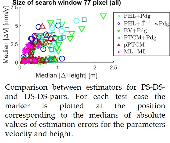
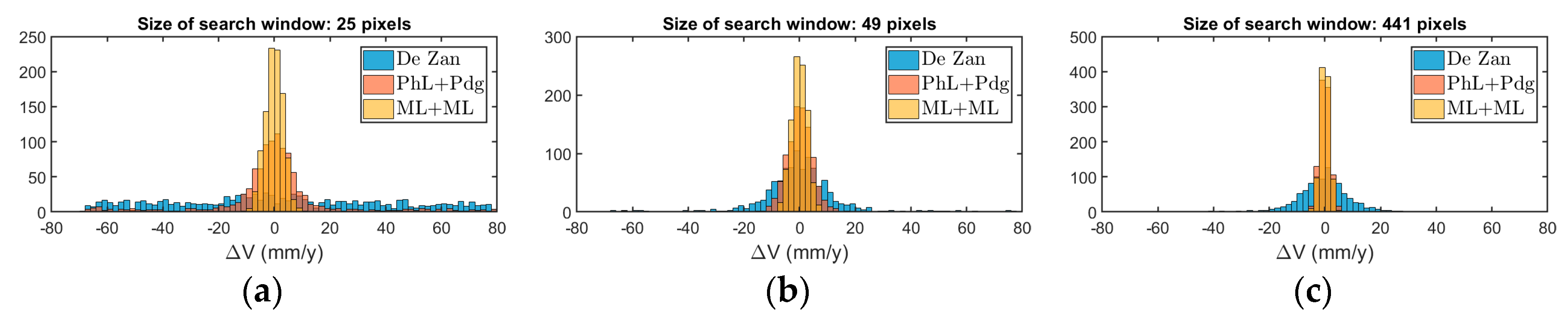
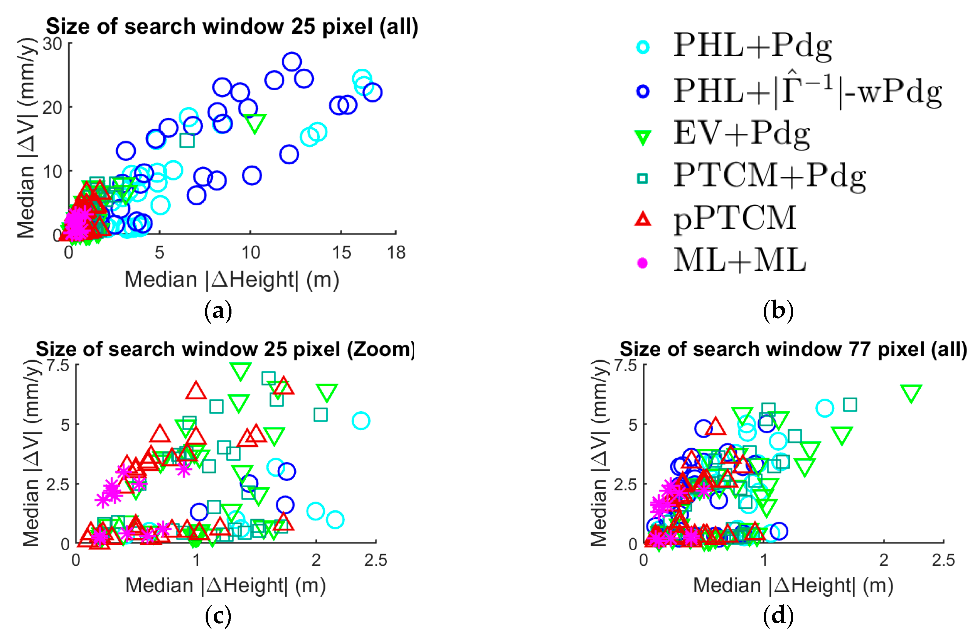
Table 1.
Settings for simulations.
| (Days) | Modifications | |
|---|---|---|
| 0.9 | 30, 45, 60, 90, 720, 1440 | - |
| 0.9 | 90 | One snow date |
| 0.9 | 60 | Two snow dates |
| 0.95 | 720 | Seasonal model = 0.05 |
| 0.9 | 60, 720 | Contaminated with 10% or 20% outliers |
© 2018 by the authors. Licensee MDPI, Basel, Switzerland. This article is an open access article distributed under the terms and conditions of the Creative Commons Attribution (CC BY) license (http://creativecommons.org/licenses/by/4.0/).
Share and Cite
MDPI and ACS Style
Even, M.; Schulz, K. InSAR Deformation Analysis with Distributed Scatterers: A Review Complemented by New Advances. Remote Sens. 2018, 10, 744. https://doi.org/10.3390/rs10050744
AMA Style
Even M, Schulz K. InSAR Deformation Analysis with Distributed Scatterers: A Review Complemented by New Advances. Remote Sensing. 2018; 10(5):744. https://doi.org/10.3390/rs10050744
Chicago/Turabian StyleEven, Markus, and Karsten Schulz. 2018. "InSAR Deformation Analysis with Distributed Scatterers: A Review Complemented by New Advances" Remote Sensing 10, no. 5: 744. https://doi.org/10.3390/rs10050744
Note that from the first issue of 2016, this journal uses article numbers instead of page numbers. See further details here.