True Orthophoto Generation from Aerial Frame Images and LiDAR Data: An Update


1
School of Civil Engineering, University College Dublin, Newstead, Belfield, Dublin 4, Ireland
2
Lyles School of Civil Engineering, Purdue University, 550 Stadium Mall Drive, West Lafayette, IN 47907-2051, USA
*
Author to whom correspondence should be addressed.
†
These authors contributed equally to this work.
Remote Sens. 2018, 10(4), 581; https://doi.org/10.3390/rs10040581
Submission received: 16 February 2018
/
Revised: 3 April 2018
/
Accepted: 5 April 2018
/
Published: 9 April 2018
(This article belongs to the Special Issue Multisensor Data Fusion in Remote Sensing)
Abstract
:Image spectral and Light Detection and Ranging (LiDAR) positional information can be related through the orthophoto generation process. Orthophotos have a uniform scale and represent all objects in their correct planimetric locations. However, orthophotos generated using conventional methods suffer from an artifact known as the double-mapping effect that occurs in areas occluded by tall objects. The double-mapping problem can be resolved through the commonly known true orthophoto generation procedure, in which an occlusion detection process is incorporated. This paper presents a review of occlusion detection methods, from which three techniques are compared and analyzed using experimental results. The paper also describes a framework for true orthophoto production based on an angle-based occlusion detection method. To improve the performance of the angle-based technique, two modifications to this method are introduced. These modifications, which aim at resolving false visibilities reported within the angle-based occlusion detection process, are referred to as occlusion extension and radial section overlap. A weighted averaging approach is also proposed to mitigate the seamline effect and spectral dissimilarity that may appear in true orthophoto mosaics. Moreover, true orthophotos generated from high-resolution aerial images and high-density LiDAR data using the updated version of angle-based methodology are illustrated for two urban study areas. To investigate the potential of image matching techniques in producing true orthophotos and point clouds, a comparison between the LiDAR-based and image-matching-based true orthophotos and digital surface models (DSMs) for an urban study area is also presented in this paper. Among the investigated occlusion detection methods, the angle-based technique demonstrated a better performance in terms of output and running time. The LiDAR-based true orthophotos and DSMs showed higher qualities compared to their image-matching-based counterparts which contain artifacts/noise along building edges.
1. Introduction
Airborne digital imaging and Light Detection and Ranging (LiDAR) systems are two leading technologies for collecting mapping data over areas of interest. Three-dimensional (3D) metric and descriptive information can be derived from aerial images using photogrammetric surface reconstruction. A key step in such 3D reconstruction is the identification of the same feature in multiple stereo images—a process referred to as image matching. With recent innovations in image matching algorithms (e.g., Semi-Global Matching (SGM) stereo method [1]) and increasing quality of airborne imaging sensors, it is possible to compute dense image-based point clouds with resolutions corresponding to the ground sampling distance (GSD) of the source images [2]. However, such point clouds suffer from the presence of outliers and occlusions, and therefore, image-based 3D point data collection is still a developing topic within the research community. Compared to image-based methods which generate point clouds indirectly, airborne LiDAR systems can directly collect 3D point data from the objects underneath. Airborne LiDAR uses a laser sensor to derive dense range data, and is equipped with Global Navigation Satellite System (GNSS) and inertial measurement unit (IMU) sensors that furnish the position and orientation of the system [3]. With recent advances in the technologies of laser, GNSS, and IMU sensors, airborne LiDAR systems can acquire reliable and accurate point clouds at a high degree of automation [4]. While the image-based point clouds posses high point density and spectral information, the 3D point data collected by LiDAR technology demonstrate a better quality in terms of occlusions and outliers.
Automated object extraction from airborne mapping data in urban areas is an important ongoing research topic. To this end, a wide range of object detection approaches have been developed for disparate applications such as 3D city modeling, map updating, urban growth analysis, and disaster management. While the quality of image-matching-based point clouds is influenced by the presence of outliers and noise, source data for many of the proposed urban object detection methods are 3D point data collected by the LiDAR technology that offers a higher geometric quality when dense point data are collected. Although high-density LiDAR point clouds possess high geometric accuracy, they lack the spectral information which is necessary to fully describe 3D surfaces. Therefore, a complete description of 3D surfaces which is essential for applications such as urban object detection and 3D city modeling cannot be provided using LiDAR point data alone. Several researchers have recommended the integration of aerial images and LiDAR, since it exploits the full benefits of complementary characteristics of both datasets [5,6,7,8]. The integrated aerial images and LiDAR data have been utilized for automated building extraction [9,10,11], 3D building modeling [12,13], and urban scene classification [14,15] with the motivation of enhancing results, increasing the degree of automation, and improving the robustness of proposed practices. Thus, accurate and reliable integration of aerial images and LiDAR data is an important requirement in several urban mapping applications.
As a prerequisite for integrating aerial images and LiDAR data, the two datasets need to be co-registered in a common reference system. Although multi-sensor aerial data collected for an area are generally registered in the same coordinate system, misalignments may exist between them due to systematic errors within the georeferencing process. As such, the datasets in question can be co-registered by utilizing either a feature-based (e.g., [16]) or an intensity-based co-registration method (e.g., [17]). Once the datasets are co-registered, the image spectral and LiDAR positional information can be related through the orthophoto generation process, which aims at linking such information by rectifying the captured aerial images for relief displacement and sensor tilt. In contrast to the original perspective images, orthophotos have a uniform scale and represent all objects in their correct planimetric locations. Therefore, besides integrating the image and LiDAR data, orthophoto generation provides an important component for geographic information system (GIS) databases. However, orthophotos generated using conventional methods suffer from an artifact known as the double-mapping effect (also referred to as ghosting effect) that occurs in areas occluded by tall objects. The double-mapping problem can be resolved through the commonly known true orthophoto generation procedure, in which an occlusion detection process is incorporated. True orthophoto generation is the most straightforward method for correctly fusing the image spectral and LiDAR positional information. Importantly, the occlusion detection process is the key prerequisite in resolving the double-mapping problem and generating true orthophotos.
This paper presents a review of occlusion detection techniques which have commonly been used for true orthophoto generation within the photogrammetric community. A comparative analysis of three of the reviewed occlusion detection methods is also presented herein. The paper also describes a framework for true orthophoto generation based on the angle-based occlusion detection technique proposed by Habib et al. [18]. To improve the performance of the angle-based method, two modifications to this technique are introduced. These modifications, which aim at resolving false visibilities reported within the angle-based occlusion detection process, are referred to as occlusion extension and radial section overlap. The impact of such modifications on the performance of the angle-based method is then verified through experimental results. A weighted averaging approach for balancing spectral information over the entire area of a true orthophoto is also proposed. Moreover, true orthophotos generated from high-resolution aerial images and high-density LiDAR data using the updated version of angle-based methodology are illustrated for two urban study areas. As mentioned earlier, dense image matching techniques have emerged as an alternative to LiDAR technology for acquiring 3D point data. Thus, to investigate the potential of such methods in producing point clouds and true orthophotos, some experiments to generate these products using the image matching technique were carried out. Accordingly, a comparison between the LiDAR-based and image matching-based true orthophotos and digital surface models (DSMs) for an urban study area is also presented in this paper.
The next section of this paper reviews the available occlusion detection and true orthophoto generation methods. In Section 3, implementation details of the angle-based occlusion detection technique are described, and the workflow of the true orthophoto generation process is discussed. The proposed modifications to the angle-based occlusion detection method and a weighted averaging method for spectral balancing are introduced in the same section. Section 4 introduces the test data employed for experiments in this study, and illustrates the experimental results. The last section concludes this study based on the utilized methods and obtained results.
2. Related Work
Orthophoto generation for an area requires four sets of input data: (1) overlapping perspective images, (2) the camera’s interior orientation parameters (IOPs), (3) the exterior orientation parameters (EOPs) of the images, and (4) an elevation model of the area in question. Traditionally, digital terrain models (DTMs) representing the bare ground have been used as elevation models for orthophoto generation [19]. Since a DTM does not represent the objects above ground, relief displacements associated with buildings and other tall objects are not fully rectified in the resulting orthophotos [20,21]. This problem can be resolved by utilizing a DSM which contains the elevations of vegetation and all objects on the ground. If the DSM is derived from LiDAR data, the image spectral and LiDAR positional information are related through the orthophoto generation process. As such, a DSM is generated from the LiDAR data by sampling the 3D points into a regular horizontal grid. Another grid with the same extent and pixel size as the raster DSM is defined to store the spectral information for the orthophoto. Each DSM cell is then projected to the corresponding perspective image by means of collinearity equations. Once the image coordinates are known for a DSM cell, the image spectral information can be assigned to the DSM cell and its equivalent pixel in the orthophoto. This method of orthophoto generation is commonly referred to as differential rectification [22], and can deliver satisfactory results in the areas where the terrain’s slope changes smoothly (e.g., in rural areas without tall structures). However, the main drawback of this technique arises when it is applied to urban areas where abrupt elevation variations exist due to the presence of buildings and other man-made objects. In dense urban centers, differentially-rectified orthophotos suffer from double-mapped areas near tall buildings and trees [23]. Such artifacts occur at the areas which are not visible in the corresponding images due to relief displacement caused by the perspective geometry. In other words, objects with lower elevation such as ground and roads are partially or fully occluded by tall buildings and trees and do not appear in the perspective images. Figure 1 shows an example of the double-mapping problem in the context of a schematic urban scene. In this figure, the areas corresponding to DSM cells D, E, and F are not visible in the image, as they have been occluded by the adjacent building. Through the differential rectification process, the DSM cells A, B, and C are projected to locations a, b, and c in the image. The spectral information of the corresponding image pixels (e.g., , , and ) are then assigned to the orthophoto pixels corresponding to A, B, and C, respectively. Additionally, due to the relief displacement caused by the building, the DSM cells in the occluded area (D, E, and F) are also projected to the image locations a, b, and c. Consequently, , , and are assigned to the orthophoto pixels at D, E, and F as well, thereby duplicating the spectral information in the generated orthophoto. This phenomenon is repeated for all the DSM cells located in the occluded area, resulting in double-mapping of the same area in the orthophoto. Figure 2 illustrates real examples of relief displacements in a perspective image, and the consequent double-mapping artifacts in the corresponding orthophoto. In Figure 2a, a portion of the perspective image is shown, where the red arrows indicate relief displacements along the building facades. As can be seen in Figure 2b, the relief displacements have been rectified in the generated orthophoto where the buildings appear in their correct orthographic locations. However, double-mapped areas enclosed by the red outlines incorrectly fill the occluded areas near the buildings. Such double-mapped areas cause a major defect and degrade the quality of the produced orthophotos. Hence, several research efforts have focused on eliminating the double-mapped areas through the true orthophoto generation process.
To produce a true orthophoto, DSM cells occluded in each image need to be identified through an occlusion detection process. Spectral information can then be assigned to orthophoto pixels corresponding to the occluded DSM cells from conjugate areas in adjacent images through a mosaicking process. Developing an efficient algorithm for occlusion detection has been the research topic of photogrammetric, computer graphics, and computer vision communities. An initial development in occlusion detection techniques is the well-known Z-buffer method [24,25], which has commonly been used within the photogrammetric community [26,27]. As demonstrated earlier, the double-mapping effect occurs when two DSM cells compete for the same location in the image (e.g., cells A and D compete for the image pixel a in Figure 1). The Z-buffer technique identifies occlusions by keeping track of the number of DSM cells projected to a given image pixel. The principle of occlusion detection using the Z-buffer method is sketched in Figure 3, where two DSM cells (A and B) compete for the same image location (pixel a). In this technique, three arrays known as the Z-buffer arrays (X, Y, and D in the figure) with the same extents as the perspective image are defined. Additionally, a visibility map with the same dimensions and cell size as the DSM is established to represent visible and occluded cells. In this example, when cell B is projected to the image, its coordinates are stored in the X and Y arrays. The distance between cell B and the perspective center is stored in the third Z-buffer array (D array). In the visibility map, the location corresponding to cell B is then marked as visible. Once cell A is projected to location a in the image, the algorithm recognizes that cell B has already been assigned to this image pixel. Among the two competing DSM cells, the closer one (A) to the perspective center is considered visible, and the other cell (B) is identified as occluded. Accordingly, the visibility map is updated to represent B as occluded and A as visible. Moreover, the Z-buffer arrays are updated to store the coordinates and distance of A instead of B.
Despite the wide use of the Z-buffer method, occlusion detection using this technique is sensitive to the image GSD and DSM cell size. This method generates false occlusion or false visibility when the image and DSM resolutions are not compatible [18,28]. False visibility is also reported in occluded areas near narrow buildings where some DSM cells do not have competing cells on the vertical surfaces of those structures. To rectify this phenomenon (referred to as the M-portion problem [26]), a digital building model (DBM) should be employed to define additional pseudo groundels along the facades/walls of narrow buildings. By also considering DBM-derived pseudo groundels on building rooftops, it is possible to mitigate the false visibility caused by incompatible image GSD and DSM cell size. Zhou et al. [29] utilized a combination of DBM and DTM instead of a raster DSM for occlusion detection using the Z-buffer method. In this approach, polygons of the building roofs from the DBM are projected to the respective perspective image. In the third Z-buffer array, the area corresponding to each polygon is filled with the rooftop distances obtained from the DBM. The distance-based criteria of the Z-buffer technique can then identify the occluded DTM cells once they are projected to the rooftop polygons in the image. DBMs have been used in further occlusion detection studies aiming at generating high-quality true orthophotos [30,31,32]. As an example, Zhou et al. [32] proposed a DBM-based approach in which occluded areas near buildings are identified based on the principle of perspective geometry. In this method, vertices of a building rooftop obtained from a DBM are projected on the ground by reconstructing the corresponding projection rays. The boundary of the occluded area near the building can then be defined using the vertices of the rooftop polygon and their projection points on the ground. Although all these authors reported satisfactory results, producing a DBM is not a straightforward task and requires additional and costly processing efforts.
To avoid the DBM generation stage and to further automatize the true orthophoto production workflow, several researchers have focused on utilizing DSMs for developing efficient occlusion detection techniques [18,28,33,34,35]. In the height-based method proposed by Habib et al. [33], the visibility of each DSM cell is analyzed by considering a search path starting from the cell in question toward the object space nadir point. The light ray connecting the perspective center to the DSM cell is referred to as the projection ray. The height of the intersection point of the projection ray with a vertical line at a given DSM location is known as the height of the projection ray at that location. Such a height value can be computed using the ray’s slope, the height of the DSM cell, and the respective horizontal distance from the DSM cell. Starting from the DSM cell toward the nadir, the height of projection ray is compared to the DSM height at regular horizontal intervals. If the DSM height is greater than the height of projection ray at a given interval, the DSM cell is considered occluded and the process terminates. Otherwise, the comparison process continues until one of the following conditions is satisfied: (1) the height of projection ray is greater than the DSM’s maximum height (i.e., maximum height along the path), or (2) all the horizontal locations are evaluated up to the nadir. In either case, the DSM cell is considered visible and the comparison process stops. Figure 4 illustrates the details of occlusion detection using the height-based method for two DSM cells (A and B). In this figure, and represent the corresponding projection rays, and d is the horizontal interval. In Figure 4a, the DSM height at the second horizontal interval () is larger than the height of (). Therefore, A is considered as an occluded cell in the visibility map and the comparison process is terminated. For the DSM cell B in Figure 4b, the height of at the fourth horizontal interval () is larger than the DSM’s maximum height (). Thus, based on condition (1), the comparison process is terminated, and cell B is flagged as visible.
In the height-gradient-based method proposed by De Oliveira et al. [34], occlusions are identified by analyzing height gradients along radial DSM profiles. Starting from the object space nadir point, height gradients between consecutive DSM cells are calculated in each radial profile. A negative gradient indicates the initial cell of an occlusion along the profile in question. Figure 5 shows a DSM profile where cell A is considered as the start of an occlusion, since there is a sudden decrease in elevation at this location. To identify the entire cells in the occluded area near the building, it is necessary to locate the last occluded cell (B in the figure). As shown in Figure 5, cell B can be identified by computing the intersection between the DSM and the line connecting A to its location in the image (pixel a). This is realized by projecting a to the DSM along the line L using the Makarovic monoplotting method [36]. However, estimating initial height values for monoplotting—which is an iterative process—imposes extra computational effort and decreases the degree of automation of the whole process. In a similar technique known as the surface-gradient-based method (SGBM) [35], a triangulated irregular network (TIN) surface is used instead of raster DSM in the occlusion detection process. The main aim of utilizing the TIN surface is to avoid the artifacts that may be generated through the interpolation process of the DSM production. It should be noted that producing a high-quality TIN which accurately represents the breaklines (e.g., building edges, roof ridge lines) may need a level of human operator intervention. In all the aforementioned studies, DSMs/DBMs required for the occlusion detection and rectification processes were derived from LiDAR point data. Currently, such surface models can also be derived from point clouds generated by dense image matching techniques [37]. However, the edges of buildings and other man-made objects cannot be reconstructed accurately using the current image matching algorithms. Such shortcomings result in the appearance of the sawtooth effect (jagged edges with sharp notches) in true orthophotos generated using the image-matching-based DSMs. To rectify the sawtooth effect, Wang et al. [38] presented an edge refinement process based on line segment matching. In this approach, corresponding 2D lines representing a building edge are extracted from an image pair. By matching the two 2D lines, a 3D line with with two fixed endpoints is reconstructed in the object space. Such 3D lines are generated for all the building edges, then discretized into individual 3D points which are added to an image-matching-based point cloud. With the assistance of the reconstructed edge points, a TIN surface that accurately represents the building edges is generated from the point cloud. As demonstrated by the authors, the improved TIN surface can then be utilized for producing a high-quality true orthophoto without the sawtooth effect.
3. Angle-Based Methodology for True Orthophoto Generation
True orthophoto generation consists of occlusion detection and mosaicking processes. To avoid the limitations associated with the reviewed techniques (Section 2), the angle-based method with two modifications is used for occlusion detection herein. To describe the details of the modifications, it is necessary to demonstrate the concept of the angle-based technique. In Section 3.1, the principle of the angle-based method for detecting occlusions along a radial DSM profile is explained and a modification referred to as occlusion extension is introduced. Section 3.2 covers the implementation details of the adaptive radial sweep technique which ensures that the visibility of entire cells within the DSM’s area of interest is checked by applying the angle-based occlusion detection procedure on sequential radial DSM profiles. To rectify the generated false visibility within the adaptive radial sweep method, a modification to this technique referred to as radial section overlap is also introduced in Section 3.2. Section 3.3 describes the true orthophoto generation process in which spectral information are assigned to occluded areas from the overlapping images. Moreover, a weighted averaging method for balancing spectral information across the entire area of a true orthophoto is proposed in Section 3.3.
3.1. Angle-Based Occlusion Detection
In the perspective projection, the top and bottom of a vertical structure are mapped to two separate locations on the image plane. The phenomenon, which is referred to as relief displacement, is the source of invisibilities/occlusions in a perspective image. Such displacement occurs in a radial direction starting from the image space nadir point toward image margins [19]. Thus, occlusions in a perspective image are proportional to the radial extent of relief displacement. In the angle-based method, occlusions are identified by sequentially analyzing the off-nadir angles of projection rays along radial directions in the DSM. Herein, the off-nadir angle to the projection ray associated with a given DSM cell is referred to as the angle [18]. Starting from the DSM cell located at the object space nadir point, the sequential angles are analyzed in each radial profile. By moving away from the nadir point in a radial profile, it is expected that the angle will increase gradually for the subsequent DSM cells if there is no occlusion within the profile in question. Accordingly, if there is an increase in the angle as one proceeds away from nadir, the corresponding DSM cells will be considered visible. Conversely, a sudden decrease of the angle when moving away from the nadir point indicates the initial cell of an occlusion. The subsequent DSM cells are then deemed occluded until the angle surpasses the angle associated with the last visible cell. As shown in Figure 6, if the angle increases while proceeding away from the nadir (N), the respective DSM cells (e.g., cells A and B) will be considered visible. In this example, the DSM cell C is identified as the first occluded cell since there is a decrease in the angle at this location (). As can be seen in the figure, the angle associated with the DSM cell D exceeds the angle of the last visible cell (B); thereby, D is deemed visible. Accordingly, the DSM cells between B and D are marked as occluded in the corresponding visibility map.
The raster DSM utilized for the occlusion detection process represents surfaces at a resolution equivalent to the square area covered by a DSM cell. Thus, such DSM does not accurately indicate the planimetric location of the boundaries of buildings and other tall objects. Due to this sampled representation, false visibility may be reported through the angle-based occlusion detection process when a high-resolution DSM (i.e., a DSM with a small cell size) is not available. An example of such false visibility is shown in Figure 7, where the DSM cells between the nadir point (N) and cell A are deemed visible since the angle is increasing for the consecutive cells in this interval. A sudden decrease in the angle occurs at B; therefore, this cell is considered as the first occluded cell. The subsequent DSM cells are deemed occluded until the angle at C exceeds the angle associated with the last visible cell (). However, the cell with the surpassing angle (C) is falsely considered visible (see visibility map 1 in Figure 7), although it is occluded by the top corner of the building. This problem arises from the fact that the raster DSM (cell A in this example) does not accurately represent the building edge. To resolve this issue, the angle of the last visible cell is incremented by a predefined value () to become larger than the angles of entire occluded cells. For example, if , it is incremented by a value to . A projection ray corresponding to the incremented angle is illustrated as a blue line in Figure 7. Accordingly, the angle of C is smaller than the extended angle of A (); thereby, cell C can now correctly be identified as occluded (see visibility map 2 in the figure). The angle increment which is referred to as occlusion extension assures that the angles of occluded cells will not exceed the angle of the last visible cell for each occlusion within a given radial profile.
3.2. Adaptive Radial Sweep Method
To investigate the visibility of the DSM cells covered by a given image, the angle-based technique is applied on successive radial profiles using the radial sweep method. Implementation of the radial sweep algorithm starts by analyzing angles along the radial direction with zero azimuth (), as shown in Figure 8 (left). After checking the visibility of DSM cells along that profile, the algorithm moves to the next radial profile by adding a predefined angular value () to the current azimuth angle (). Accordingly, the DSM is swept by defining the subsequent radial profiles and applying the angle-based method along them. A visibility map with the same extent and cell size as the DSM is defined to flag the visible/occluded DSM cells. Using the DSM cell size and , an R to array is created in which R is the radial distance from nadir and is the azimuth angle for a given radial profile, as shown in Figure 8 (right). The R to array is used to store the angle associated with each DSM cell along the corresponding radial profile. Moreover, two arrays with the same extents and cell size as the R to array are defined to store the X and Y coordinates of the DSM cells. For each DSM cell, the respective R, , and values are calculated. The computed R and values may not correspond to the sampled values in the corresponding R to array elements. Thus, the calculated angle is stored in the closest location in the R to array. At the same time, the X and Y coordinates of the DSM cell are stored in the corresponding locations in X and Y arrays, respectively. After computing angles for entire DSM cells, the occlusion detection process starts by checking the computed angles along each radial profile in the R to array. Accordingly, the visible and occluded locations along each profile are stored in the visibility map using the respective coordinates available in the X and Y arrays.
Defining the azimuth increment value () is a crucial step in the implementation of the radial sweep method. Choosing a small value for will lead to reanalyzing the DSM cells close to nadir repeatedly, thereby increasing the computational time. Furthermore, selecting a large value for will result in unvisited DSM cells at the boundaries. Therefore, should be defined in a way that on the one hand will not result in revisited DSM cells, and on the other will not leave marginal DSM cells unvisited. This can be accomplished through the adaptive radial sweep method, in which is decreased while the radial distance from nadir increases. In this technique, the DSM is partitioned into concentric radial sections centered at the object space nadir point (N) as shown in Figure 9 (left). Accordingly, the corresponding R to array is divided in the R direction as illustrated in Figure 9 (right). In the R to array, cell size in the radial direction can be considered equal to the DSM cell size for all the sections. As can be seen in Figure 9 (left), decreases for the sections while the radial distance (R) increases. Thus, the number of rows in the R to array becomes larger for the corresponding sections with the increase of R as shown Figure 9 (right). The number of radial sections and values are defined based on the DSM’s area covered by the corresponding image and the DSM cell size. For each radial section, can be set to a value so that the sectorial distance between subsequent radial profiles at the outer margin of that section will not be larger than the DSM cell size.
The DSM partitioning within the adaptive radial sweep method optimizes the computational aspect of the occlusion detection process. However, assuming that each radial section is processed independently from the previous/next section, such partitioning may lead to reporting false visibility in some occluded areas with large radial extensions. Figure 10 shows a schematic example of such false visibility for a DSM profile and illustrates the details of resolving this issue. In Figure 10a, the border of two radial sections ( and ) is located within an occluded area near the building (at cell B). Using the first radial section (), the occlusion detection process starts from the object space nadir point (N) up to the DSM cell B. Having cell A as the last visible cell, the cells between A and B (including B) are correctly considered as occluded. However, the occlusion detection using the second radial section () commences at B; thereby, B is wrongly considered as visible. Moreover, since the angle for the subsequent DSM cells increases gradually, the DSM cells between B and C (including C) are also incorrectly considered as visible. To mitigate this issue, an overlap should be considered between the two sequential radial sections within the adaptive radial sweep method. As shown in Figure 10b, the second radial section () is defined to cover an area in the first radial section (). As such, the second radial section starts at a DSM location (cell ) closer to the nadir point. Starting from , the angle is computed for the sequential DSM cells to find the last visible cell before the occlusion. By comparing the angles of the cells after A with , the occluded DSM cells are correctly identified as shown in Figure 10b.
3.3. True Orthophoto Mosaic Generation
To generate a true orthophoto mosaic using multiple overlapping images, it is first necessary to identify the occluded/visible DSM cells in each perspective image. Figure 11 shows the results of occlusion detection using the adaptive radial sweep method for an image. In Figure 11a, an orthophoto generated from the perspective image using the differential rectification method is illustrated. The orange portions represent the detected occlusions which cover the double-mapped areas in the orthophoto. For this example, the DSM area covered by the image was divided into three radial sections through the adaptive radial sweep method. In this figure, the cyan point represents the object space nadir point (N), and the green circle is the first radial section. The area between the red circles is the second radial section, and the portion between the blue circles is the third radial section. Figure 11b shows the corresponding visibility map, where magenta areas represent the DSM cells which are visible in the perspective image. After identifying occlusions in each image, spectral information can be assigned to occluded portions from adjacent overlapping images through a mosaicking process.
Having generated visibility maps for the overlapping images, it is feasible to identify the DSM cells which are visible/occluded in each image. If a DSM cell is occluded in an image, adjacent images from which that DSM cell is visible are identified by checking the respective visibility maps. As a basic mosaicking approach, spectral information can be assigned to the orthophoto pixel corresponding to the occluded cell from the closest visible image. As such, horizontal distances between the DSM cell and perspective centers of visible images are computed to find the closest image. The DSM cell is then projected to that image using the respective IOPs and EOPs by means of collinearity equations. The spectral information of the corresponding image pixel is then assigned to the respective orthophoto pixel. The closest visible image identification and projection processes are repeated for the entire DSM cells until appropriate spectral information is derived for all orthophoto pixels. This mosaicking approach ensures the occluded areas are filled by correct spectral information, thereby avoiding the double-mapping problem. However, spectral dissimilarity may appear in the true orthophoto since the images might be taken in different lighting conditions. Such spectral discontinuities (known as seamlines) take place at the borders of image portions in the true orthophoto. Figure 12a shows the contribution of images to part of a true orthophoto generated using the closest visible image criteria. In this figure, each color represents an area for which spectral information has been derived from an individual image. The random colors clarify that in an area covered by a closest image (e.g., the light green portion), spectral information for occluded portions are derived from neighboring closest images. Filling such occluded portions from the adjacent images (i.e., especially images form the neighboring flight lines) may also lead to spectral dissimilarity. Some studies have been carried out to adjust the spectral information along seamlines appearing in true orthophotos. As an example, De Oliveira et al. [35] considered a buffer area around each seamline and blended the spectral information of the involved images using a weighted averaging method. Although this approach mitigates the seamline effect, the color transition takes place within a narrow buffer area along each seamline. Moreover, this method does not address the spectral variations at the border of occluded areas. As such, a weighted averaging method is proposed to balance the spectral information over the entire area of the true orthophoto. In this approach, spectral information for each orthophoto pixel is sampled from all the visible images using the inverse distance weighting (IDW) method proposed by Shepard [39]. If n is a set of images from which a DSM cell is visible, spectral information for the corresponding orthophoto pixel (e.g., ) is computed from the spectral information of those images as:
where for , is the spectral information of the corresponding pixel in each visible image, is the contribution weight of the image in question given by Equation (2), and is the horizontal distance between the DSM cell and the perspective center of the image.
Based on Equation (2), weight of each visible image decreases as the distance of its perspective center from the DSM cell increases. Figure 12b illustrates the contribution of images in the IDW-based spectral balancing process for the area of Figure 12a using the same random colors. As represented by the corresponding colors in this figure, the contribution of each image is greater at the areas closer to its perspective center. This IDW-based averaging approach blends the spectral information from multiple visible images, thereby avoiding the appearance of seamlines in the true orthophoto. It also decreases the spectral dissimilarity that may appear at the border of occluded areas. Moreover, it decreases the artifacts associated with moving objects (i.e., cars, pedestrians), since the spectral information for each orthophoto pixel is sampled from multiple sky locations.
4. Experimental Results
In this section, the aerial imagery and LiDAR datasets utilized for the experiments within this study are introduced, and the respective experimental results are presented and discussed. Section 4.1 describes the test data and provides the specifications of the airborne sensors employed for the data acquisition. In Section 4.2, the impact of the modifications to the angle-based methodology is illustrated using the experimental results. Section 4.3 presents a comparative analysis of occlusion detection results from the Z-buffer, height-based, and angle-based techniques. In Section 4.4, true orthophotos generated using the angle-based methodology are illustrated and discussed. Section 4.5 presents a comparison between the LiDAR-based and image-matching-based true orthophotos and DSMs. In this study, the developed algorithms were implemented in C++ using OpenCV [40]. The running times reported within this section were obtained on a 64-bit Windows 10 PC with an Intel(R) Core(TM) i7-3770 CPU @ 3.40 GHz, 4-core processor, with 32 GB memory.
4.1. Test Data and Study Areas
For this study, a set of aerial images and a LiDAR dataset for an area of approximately 2 km2 in the city center of Dublin, Ireland, were available [41]. Data acquisition was carried out by an AS355 helicopter at an average flying altitude of 300 m above ground level (AGL) on March 2015, using the flight path proposed by Hinks et al. [42]. Based on that study, airborne LiDAR data suitable for urban modeling tasks could be acquired using two sets of parallel flight lines perpendicular to each other, which are oriented from the street layout (see Figure 13a). As shown in Figure 13b, a 67% overlap between adjacent strips should also be considered to ensure data capture on building facades and other vertical surfaces. Such arrangements, along with a low flight altitude, increase the sampling density on the captured surfaces. The LiDAR datasets collected using this flight pattern are highly beneficial for 3D building modeling and visualizing complex urban scenes [43].
Table 1 provides the specifications of the utilized LiDAR system and the collected LiDAR data. To acquire this dataset, the 67% strip overlap recommended by Hinks et al. [42] was slightly increased (to 70%) to avoid lacuna in the data. Based on the orientation of Dublin streets, the flight path included two sets of flight lines in two perpendicular directions: (1) northwest to southeast, and (2) northeast to southwest. Total number of flight lines was 41, from which 21 flight lines were in the northwest to southeast direction, and 20 flight lines were along the northeast to southwest direction. The LiDAR dataset was delivered as 356 square tiles (100 m × 100 m) in LAS [44] format version 1.2.
The aerial images were acquired from the same platform as the LiDAR data, also using the flight pattern that was explained earlier. Specifications of the utilized imaging sensor and the collected images are summarized in Table 2.
In the region covered by the LiDAR and imagery datasets, two study areas were selected to conduct experiments: (1) Trinity College Dublin, and (2) Dawson Street. Each study area covered a 400 m × 300 m rectangular region, for which a raster DSM with 10 cm cell size was generated from the LiDAR data. Sampling the LiDAR point data into a raster DSM starts with partitioning the -plane enclosing the points into square cells. The height values are then assigned to the cells by mapping the 3D point data into the DSM’s horizontal grid. Due to the irregular distribution of LiDAR data, some DSM cells have more than one LiDAR point while some cells remain empty without being assigned height values. In the case of more than one point per cell, the maximum height of the points appearing in each cell is assigned to the cell in question. In this study, height values for the empty DSM cells were computed using the IDW method, by interpolating the ground and non-ground surfaces separately as proposed by Gharibi [45]. Accordingly, the empty DSM cells are first roughly interpolated using the interpolation on paths technique [1] to derive a temporary DSM. Next, the temporary DSM is classified to ground and non-ground classes using the approach proposed by Tarsha-Kurdi et al. [46]. Finally, the empty DSM cells are accurately interpolated using the IDW method by utilizing the non-ground class as a constraint to separate the interpolation process between the ground and non-ground surfaces. The DSMs generated using this approach for the Trinity College and Dawson Street study areas are shown in Figure 14a,b, respectively. These DSMs along with images covering the two study areas were used in the occlusion detection and true orthophoto generation experiments herein.
4.2. Impact of Modifications to the Angle-Based Method
Having introduced the details of occlusion extension within the angle-based method, this section presents a real example of the impact of such modification on the occlusion detection results. As mentioned in Section 3.1, the grid-based representation of surfaces in raster DSMs may result in reporting false visibility within the the angle-based occlusion detection process. This problem commonly occurs when a high-resolution DSM (i.e., with a cell size equal to or less than 10 cm) is not available for the study area. Therefore, to illustrate this problem and to demonstrate the impact of the occlusion extension, a DSM with 20 cm cell size was generated for the Trinity College study area in addition to the DSM with 10 cm cell size.This DSM and a perspective image were used to perform the differential rectification and occlusion detection experiments, whose results are shown in Figure 15. In Figure 15a, the detected occlusions (orange portions) before considering the occlusion extension are visualized on a differentially-rectified orthophoto. Since the DSM with 20 cm cell size does not represent the building edges accurately, false visibilities can be observed on the outer edges of the occluded area, as indicated by the red arrows. To rectify this problem, a was added to the angle of the last visible cells through the angle-based occlusion detection process. As can be seen in Figure 15b, the introduced occlusion extension successfully rectified the false visibilities.
As explained in Section 3.2, DSM partitioning within the adaptive radial sweep method may cause false visibility when the border of two radial sections is inside an occluded area. In the same section, it was proposed that considering an overlap between successive radial sections resolves the issue of false visibility. Figure 16 presents a real example of such false visibility, as well as the rectification of false visibility by having an overlap between the sequential radial sections. In Figure 16a, the detected occlusions (orange portions) using the adaptive radial sweep method are shown on a differentially-rectified orthophoto. The cyan curve in this figure is the border of radial sections which do not have any overlap. As can be seen in this figure, the detected occlusions have filled the double-mapped areas in the orthophoto. However, at three portions inside the second radial section, false visibilities can be observed, as indicated by the red arrows. Figure 16b illustrates the occlusion detection result for the same area when an overlap of 5 m was considered between the two radial sections. The cyan curve in this figure is the end of the first radial section, and the red curve represents the start of the second radial section. As can be seen in this figure, the three portions of false visibilities shown in Figure 16a were rectified. The amount of overlap between the radial section can be selected based on the radial extents of occlusions (i.e., or relief displacements) within the study area.
4.3. Comparison of the Occlusion Detection Techniques
In addition to the angle-based occlusion detection method, the Z-buffer and height-based techniques were also implemented in this study. To compare and evaluate the performance of these methods, some occlusion detection experiments were carried out. Figure 17 compares the identified occlusions using the Z-buffer and angle-based techniques for a perspective image. A portion of the image is shown in Figure 17a, where relief displacements can be observed along the building walls. Figure 17b illustrates an orthophoto generated from the image using the differential rectification method. As can be seen in this figure, double-mapped portions occupy the occluded areas caused by the relief displacements at the building location. In Figure 17c, the pink portions indicate the detected occlusions using the Z-buffer method, visualized on the differentially-rectified orthophoto. A closer look at this figure reveals that occlusions were not fully detected due to the limitations of the Z-buffer method, and false visibilities can be observed in the occluded areas. In Figure 17d, the orange areas indicate the identified occlusions using the angle-based technique. Comparing Figure 17c,d, one can see that the angle-based approach fully identified the occluded areas.
Figure 18 presents the occlusion detection results from the height-based and angle-based methods for another perspective image. Figure 18a shows part of the image, and Figure 18b illustrates the corresponding differentially-rectified orthophoto. In Figure 18c, the pink areas indicate the identified occlusions using the height-based technique. For this experiment, the horizontal interval within the height-based method was set equal to the DSM cell size (d = 10 cm). In Figure 18d, orange portions show the detected occlusions using the angle-based technique. A comparison of Figure 18c,d shows that the height-based method detected almost all the occlusions. However, the running time of the height-based algorithm was longer than the angle-based algorithm. Table 3 provides running times of the Z-buffer, height-based, and angle-based algorithms for occlusion detection using one of the perspective images and a DSM with 10 cm cell size. The perspective image covered 7,904,581 DSM cells, which were checked by the respective occlusion detection algorithms. As can be seen from Table 3, the Z-buffer method had the shortest running time among the tested algorithms. Nevertheless, the Z-buffer technique was not capable of detecting occlusions entirely, as demonstrated earlier (see Figure 17c). While the height-based method could achieve the same results for occlusion detection as the angle-based technique, the processing time of this method was almost double that of the angle-based algorithm. The height-based occlusion detection process is longer since for analyzing the visibility of each DSM cell, the DSM height values at several horizontal intervals must be compared to the height of the corresponding projection ray. As reported in Table 3, the running times of these methods for detecting occlusions in a single image are in terms of seconds. However, the time differences can be significant when generating true orthophoto for a large area, for which hundreds of perspective images must be processed.
4.4. LiDAR-Based True Orthophotos
Using both the closest visible image and IDW-based spectral balancing methods, experiments for generating true orthophoto for the Trinity College and Dawson Street study areas were conducted. Additionally, orthophotos using the differential rectification method were generated for the two study areas. To demonstrate the importance of the occlusion detection process, Figure 19 compares an orthophoto generated using the differential rectification technique with a true orthophoto produced using the closest visible image criteria. Figure 19a shows the differentially-rectified orthophoto in which spectral information was assigned to each DSM cell from the closest image, irrespective of whether the cell in question was visible in the image or not. As indicated by the red arrows, double-mapped portions filled the areas which are not visible in the corresponding closest images. In Figure 19b, a true orthophoto produced by carrying out the angle-based occlusion detection process is illustrated. In this orthophoto, pixels corresponding to the DSM cells that are occluded in the respective closest images are shown in orange. Figure 19c presents a true orthophoto generated using the closest visible image mosaicking approach. As can be seen in in this figure, the occluded areas were correctly filled with spectral information from conjugate areas in the closest visible adjacent images. In Figure 19d, the contribution of images to the true orthophoto is visualized using random colors. Each color represents an area to which the spectral information was assigned from an individual image. The colors clarify that in an area covered by an image (e.g., the red portion), spectral information for occluded portions was derived from neighboring images identified as closest visible images.
Figure 20 compares the true orthophotos generated using the closest visible image criteria (Figure 20a,c) with the ones produced through the IDW-based spectral balancing process (Figure 20b,d). As pointed by the arrow in Figure 20a, a diagonal seamline appeared in the true orthophoto because images in one flight line were taken in cloudy weather, while images in the adjacent flight line were collected in sunlight. As can be seen in Figure 20b, the spectral dissimilarity was rectified in the true orthophoto generated using the IDW-based color balancing approach. As described in Section 3.3, sampling the spectral information from different camera locations results in lower visibility of moving objects such as pedestrians and vehicles in the generated true orthophoto. This phenomenon, which gives a cleaner look to the true orthophoto, can be observed by comparing Figure 20c,d. The red arrows in Figure 20c indicate pedestrians which are absent in Figure 20d, where spectral information for each orthophoto pixel was sampled from several images collected from different flight lines.
In Figure 21, results of true orthophoto generation using the IDW-based color balancing method for the Trinity College and Dawson Street study areas are shown. Figure 21a,c present the true orthophotos for the entire region of the two study areas. In these figures, all the buildings appear in their correct planimetric locations, double-mapped areas do not exist, and spectral discontinuities are compensated. Figure 21b provides a closer look at the portion enclosed by the red rectangle in Figure 21a, which corresponds to the area that was previously shown in Figure 17. Considering Figure 17d, one can see that occluded areas are now filled with correct spectral information in Figure 21b. Figure 21d provides a close-up of the area shown by the red rectangle in Figure 21c, which is identical to the portion that was previously presented in Figure 18. The Trinity College and Dawson Street study areas were fully or partially covered by 98 and 101 perspective images, respectively. These images along with the respective DSMs (shown in Figure 14) were utilized for generating the true orthophotos shown in Figure 21a,c. It should be noted that each perspective image with 9000 × 6732 pixels frame size (see Table 2) occupies on average 86 MB (i.e., in PNG format) on the hard drive. Table 4 provides the running times of orthophoto and true orthophoto production processes for the two study areas. The third column in the table presents the processing time of orthophoto generation using the differential rectification method. The fourth and the fifth columns titled as True orthophoto 1 and 2 show the running times of true orthophoto production using the closest visible image and IDW-based spectral balancing approaches, respectively. The running time of orthophoto production is a fraction of the true orthophoto generation’s execution times (e.g., by comparing the third and forth columns). This time difference points out the consumed time for the angle-based occlusion detection process within the true orthophoto generation stage. Moreover, the difference between the fourth and fifth columns indicates the computational time of the IDW-based color balancing process.
As reviewed in Section 2, significant efforts have been carried out within the research community for the development of occlusion detection methods to automatize the true orthophoto generation process. However, the developed techniques have yet to be commercialized, and the photogrammetric industry still lacks a software package that enables true orthophoto generation automatically. Using available software programs (e.g., Inpho [47] by Trimble, TerraPhoto [48] by Terrasolid), a true orthophoto can be produced only when a DBM of the corresponding area is available. Such software packages can automatically rectify images for scale variation and perspective projection using a DTM, thereby generating an orthophoto with uniform scale. However, relief displacements are not fully rectified in such an orthophoto, since the DTM does not include the objects above ground. To compare such DTM-based orthophotos with true orthophotos, the Trinity College and Dawson Street datasets were processed using the TerraPhoto software. Figure 22 presents the corresponding results along with the true orthophotos generated using the IDW-based color balancing approach. In Figure 22a,c, two parts of the true orthophotos are shown, and Figure 22b,d illustrate the DTM-based orthophotos generated using TerraPhoto. As indicated by the red arrows, relief displacements can be observed in the orthophotos shown in Figure 22b,d.
4.5. LiDAR-Based versus Image-Matching-Based Products
To compare the LiDAR-based true orthophotos and DSMs with the same products generated by image matching, the Trinity College dataset was processed with Pix4Dmapper [49] by Pix4D. As mentioned earlier, the Trinity College dataset included dense LiDAR data and 98 high-resolution aerial images. The images and their accurate EO parameters were used as input for the image matching process in the Pix4D software. By processing the data with Pix4D, a dense point cloud and a high-resolution true orthophoto (10 cm pixel size) were generated. Figure 23 illustrates two examples of the Trinity College LiDAR-based and image-matching-based true orthophotos with a pixel size equal to 10 cm. In Figure 23a, part of the LiDAR-based orthophoto is shown where correct spectral values were assigned to the top roof of the building and to the ground. Figure 23b presents the true orthophoto generated by the image matching technique for the same area. A closer look at this figure reveals that the outer part of the building boundary (pointed by the red arrows) does not have correct spectral information. Figure 23c shows another portion of the LiDAR-based true orthophoto, and Figure 23d illustrates the corresponding part of the image-matching-based true orthophoto. Compared with the LiDAR-based true orthophoto (Figure 23c), this product (Figure 23d) contains a sawtooth effect [38] along the building edges. Such artifacts degrade the quality of the image-matching-based true orthophoto and hamper its reliable usage in urban mapping applications.
To evaluate the geometric aspects of the image-matching-based point cloud, a DSM with 10 cm cell size was generated from this point cloud. Figure 24 illustrates the LiDAR-based and image-matching-based DSMs for two buildings in the Trinity College study area. In Figure 24a, a portion of the LiDAR-based DSM is shown, and Figure 24b illustrates the image-matching-based DSM for the same area. As can be seen in Figure 24b, the image-matching-based DSM contains noise and outliers along the building edges. This problem also appears at the building edges for another portion of the image-matching-based DSM shown in Figure 24d. Such noise and outliers are the main reasons for the appearance of the sawtooth effect in the image-matching-based true orthophotos. To produce true orthophotos without the sawtooth effect, it is necessary to enhance the noisy edges in the image-matching-based DSMs. Comparing the LiDAR-based DSMs (Figure 24a,c) with the image-matching-based products (Figure 24b,d), one can see that LiDAR-based DSMs are cleaner and represent the building boundaries accurately. This is true based upon the availability of high-density LiDAR data (e.g., the LiDAR dataset utilized herein).
5. Conclusions
The availability of 3D point data with spectral information is highly beneficial in applications such as urban object detection and 3D city modeling. Point clouds generated by image matching techniques possess the image spectral information in addition to the 3D positional data. However, without enhancement, utilizing such point clouds in urban mapping applications is still hampered by the presence of occlusions, outliers, and noise—especially along building edges. Alternatively, 3D point data with spectral information for an area can be achieved by integrating aerial images and LiDAR data collected for the area in question. True orthophoto generation is an efficient way to fuse the image spectral and LiDAR positional information. Moreover, true orthophotos are valuable products for decision-making platforms such as GIS environments. The most important prerequisite in the true orthophoto generation process is the identification of occlusions in the collected images.
This paper reviewed the occlusion detection techniques which have been utilized for true orthophoto generation within the photogrammetric community. The limitations/advantages of these methods were described in Section 2, and a comparative analysis of three techniques was provided in Section 4. Among the investigated occlusion detection methods, the angle-based technique to which two modifications were introduced in this paper demonstrated a satisfactory performance in terms of output and running time. Thus, a workflow for true orthophoto generation based on the angle-based occlusion detection technique was described in the paper. A color balancing approach based on the IDW method was also introduced to mitigate the seamline effect and spectral discontinuity that may appear in true orthophotos. Results of true orthophotos generation from high-resolution aerial images and high-density LiDAR data for two urban study areas were then presented. The utilized airborne datasets for the experiments within this study, were acquired using a special flight path setting resulting in very high-density LiDAR data (horizontal point density = 300 pt/m2) and high-resolution images (image GSD = 3.4 cm). To the best of our knowledge, an experimental study on different aspects of true orthophoto generation using such high-resolution airborne datasets has not been reported previously. Moreover, the LiDAR-based true orthophotos and DSMs were compared with the same products generated using the image matching technique. It was demonstrated that the image-matching-based true orthophotos and DSMs contained the sawtooth effect and outliers along building edges, and without refinement cannot reliably be used in urban mapping tasks.
True orthophoto generation addresses the fusion of image spectral and LiDAR positional information based on a 2.5-dimensional (2.5D) DSM. Therefore, the true orthophoto generation process described within this paper cannot assign spectral information to LiDAR point data on vertical surfaces. Accordingly, future research can focus on devising an approach for assigning the image spectral information to the LiDAR point data on vertical surfaces. Future research can also concentrate on developing methods refining non-ground edges in the image-matching-based point clouds or on improving the performance of the relevant algorithms for reconstructing the edges accurately.
Acknowledgments
This work was funded by European Research Council grant ERC-2012-StG_20111012 “RETURN-Rethinking Tunnelling in Urban Neighbourhoods” Project 307836.
Author Contributions
Hamid Gharibi and Ayman Habib conceived the study and conducted the experiments. Hamid Gharibi implemented the algorithms, processed the data, and generated the results under Ayman Habib’s supervision. Hamid Gharibi wrote the manuscript, and Ayman Habib edited and revised the manuscript.
Conflicts of Interest
The authors declare no conflict of interest.
References
- Hirschmüller, H. Stereo processing by semiglobal matching and mutual information. IEEE Trans. Pattern Anal. Mach. Intell. 2008, 30, 328–341. [Google Scholar] [CrossRef] [PubMed]
- Haala, N.; Rothermel, M. Image-Based 3D Data Capture in Urban Scenarios; Photogrammetric Week ’15; Wichmann/VDE Verlag: Berlin/Offenbach, Germany, 2015; pp. 119–130. [Google Scholar]
- Wehr, A.; Lohr, U. Airborne laser scanning—An introduction and overview. ISPRS J. Photogramm. Remote Sens. 1999, 54, 68–82. [Google Scholar] [CrossRef]
- Vosselman, G.; Mass, H.G. Airborne and Terrestrial Laser Scanning; Whittles Publishing: Dunbeath, UK, 2010. [Google Scholar]
- Rottensteiner, F.; Trinder, J.; Clode, S.; Kubik, K. Using the Dempster-Shafer method for the fusion of LIDAR data and multi-spectral images for building detection. Inf. Fus. 2005, 6, 283–300. [Google Scholar] [CrossRef]
- Kim, C.; Habib, A. Object-based Integration of Photogrammetric and LiDAR Data for Accurate Reconstruction and Visualization of Building Models. Sensors 2009, 9, 5679–5701. [Google Scholar] [CrossRef] [PubMed]
- Khoshelham, K.; Nardinocchi, C.; Frontoni, E.; Mancini, A.; Zingaretti, P. Performance evaluation of automated approaches to building detection in multi-source aerial data. ISPRS J. Photogramm. Remote Sens. 2010, 65, 123–133. [Google Scholar] [CrossRef]
- Kwak, E.; Habib, A. Automatic 3D Building Model Generation From Lidar and Image Data Using Sequential Minimum Bounding Rectangle. Int. Arch. Photogramm. Remote Sens. Spatial Inf. Sci. 2012. [Google Scholar] [CrossRef]
- Awrangjeb, M.; Ravanbakhsh, M.; Fraser, C.S. Automatic detection of residential buildings using LIDAR data and multispectral imagery. ISPRS J. Photogramm. Remote Sens. 2010, 65, 457–467. [Google Scholar] [CrossRef]
- Awrangjeb, M.; Zhang, C.; Fraser, C.S. Automatic extraction of building roofs using LIDAR data and multispectral imagery. ISPRS J. Photogramm. Remote Sens. 2013, 83, 1–18. [Google Scholar] [CrossRef]
- Gilani, S.A.N.; Awrangjeb, M.; Lu, G. An Automatic Building Extraction and Regularisation Technique Using LiDAR Point Cloud Data and Orthoimage. Remote Sens. 2016, 8, 258. [Google Scholar] [CrossRef]
- Habib, A.F.; Zhai, R.; Kim, C. Generation of Complex Polyhedral Building Models by Integrating Stereo-Aerial Imagery and Lidar Data. Photogramm. Eng. Remote Sens. 2010, 76, 609–623. [Google Scholar] [CrossRef]
- Arefi, H.; Reinartz, P. Building reconstruction using DSM and orthorectified images. Remote Sens. 2013, 5, 1681–1703. [Google Scholar] [CrossRef] [Green Version]
- Guo, L.; Chehata, N.; Mallet, C.; Boukir, S. Relevance of airborne lidar and multispectral image data for urban scene classification using Random Forests. ISPRS J. Photogramm. Remote Sens. 2011, 66, 56–66. [Google Scholar] [CrossRef]
- Gerke, M.; Xiao, J. Fusion of airborne laserscanning point clouds and images for supervised and unsupervised scene classification. ISPRS J. Photogramm. Remote Sens. 2014, 87, 78–92. [Google Scholar] [CrossRef]
- Habib, A.; Jarvis, A.; Kersting, A.P.; Alghamdi, Y. Comparative analysis of georeferencing procedures using various sources of control data. Int. Arch. Photogramm. Remote Sens. Spat. Inf. Sci. 2008, 37, 1147–1152. [Google Scholar]
- Parmehr, E.G.; Fraser, C.S.; Zhang, C.; Leach, J. Automatic registration of optical imagery with 3d lidar data using local combined mutual information. ISPRS J. Photogramm. Remote Sens. 2014, 88, 28–40. [Google Scholar] [CrossRef]
- Habib, A.F.; Kim, E.M.; Kim, C.J. New Methodologies for True Orthophoto Generation. Photogramm. Eng. Remote Sens. 2007, 73, 25–36. [Google Scholar] [CrossRef]
- Mikhail, E.M.; Bethel, J.S.; McGlone, J.C. Introduction to Modern Photogrammetry; John Wiley & Sons, Inc.: New York, NY, USA, 2001. [Google Scholar]
- Günay, A.; Arefi, H.; Hahn, M. Semi-automatic true orthophoto production by using LIDAR data. In Proceedings of the International Geoscience and Remote Sensing Symposium (IGARSS), Barcelona, Spain, 23–28 July 2007; pp. 2873–2876. [Google Scholar]
- Barazzetti, L.; Brovelli, M.; Scaioni, M. Generation of true-orthophotos with lidar high resolution digital surface models. Photogramm. J. Finl. 2008, 21, 26–36. [Google Scholar]
- Novak, K. Rectification of Digital Imagery. Photogramm. Eng. Remote Sens. 1992, 58, 339–344. [Google Scholar]
- Skarlatos, D. Orthophotograph Production in Urban Areas. Phtogramm. Rec. 1999, 16, 643–650. [Google Scholar] [CrossRef]
- Catmull, E.E. A Subdivision Algorithm for Computer Display of Curved Surfaces. Ph.D. Thesis, The University of Utah, Salt Lake City, UT, USA, 1974. [Google Scholar]
- Ahmar, F.; Jansa, J.; Ries, C. The generation of true orthophotos using a 3D building model in Conjunction with a conventional dtm. Iaprs 1998, 32, 16–22. [Google Scholar]
- Rau, J.; Chen, N.Y.; Chen, L.C. True Orthophoto Generation of Built-Up Areas Using Multi-View Images. Photogramm. Eng. Remote Sens. 2002, 68, 581–588. [Google Scholar]
- Sheng, Y.; Gong, P.; Biging, G.S. True Orthoimage Production for Forested Areas from Large-Scale Aerial Photographs. Photogramm. Eng. Remote Sens. 2003, 69, 259–266. [Google Scholar] [CrossRef]
- Sheng, Y. Minimising algorithm-induced artefacts in true ortho-image generation: A direct method implemented in the vector domain. Photogramm. Rec. 2007, 22, 151–163. [Google Scholar] [CrossRef]
- Zhou, G.; Schickler, W.; Thorpe, A.; Song, P.; Chen, W.; Song, C. True orthoimage generation in urban areas with very tall buildings. Int. J. Remote Sens. 2004, 25, 5163–5180. [Google Scholar] [CrossRef]
- Chen, L.C.; Teo, T.A.; Wen, J.Y.; Rau, J.Y. Occlusion-Compensated True Orthorectification for High-Resolution Satellite Images. Photogramm. Rec. 2007, 22, 39–52. [Google Scholar] [CrossRef]
- Deng, F.; Kang, J.; Li, P.; Wan, F. Automatic true orthophoto generation based on three-dimensional building model using multiview urban aerial images. J. Appl. Remote Sens. 2015, 9, 095087. [Google Scholar] [CrossRef]
- Zhou, G.; Wang, Y.; Yue, T.; Ye, S.; Wang, W. Building Occlusion Detection from Ghost Images. IEEE Trans. Geosci. Remote Sens. 2017, 55, 1074–1084. [Google Scholar] [CrossRef]
- Habib, A.; Bang, K.; Kim, C.; Shin, S. True Ortho-Photo Generation from High Resolution Satellite Imagery; Springer: Berlin, Germany, 2006; pp. 641–656. [Google Scholar]
- De Oliveira, H.C.; Galo, M.; Dal Poz, A.P. Height-Gradient-Based Method for Occlusion Detection in True Orthophoto Generation. IEEE Geosci. Remote Sens. Lett. 2015, 12, 2222–2226. [Google Scholar] [CrossRef]
- De Oliveira, H.C.; Porfírio Dal Poz, A.; Galo, M.; Habib, A.F. Surface Gradient Approach for Occlusion Detection Based on Triangulated Irregular Network for True Orthophoto Generation. IEEE J. Sel. Top. Appl. Earth Obs. Remote Sens. 2018, 11, 443–457. [Google Scholar] [CrossRef]
- Radwan, M.; Makarovic, B. Digital mono-plotting system-improvements and tests. ITC J. 1980, 3, 511–533. [Google Scholar]
- Haala, N. Multiray Photogrammetry and Dense Image Matching; Photogrammetric Week ’11; Wichmann/VDE Verlag: Berlin/Offenbach, Germany, 2011; pp. 185–195. [Google Scholar]
- Wang, Q.; Yan, L.; Sun, Y.; Cui, X.; Mortimer, H.; Li, Y. True orthophoto generation using line segment matches. Photogramm. Rec. 2018. [Google Scholar] [CrossRef]
- Shepard, D. A two-dimensional interpolation function for irregularly-spaced data. In Proceedings of the 1968 ACM National Conference, New York, NY, USA, 27–29 August 1968; pp. 517–524. [Google Scholar]
- OpenCV. Open Source Computer Vision Library. Available online: https://opencv.org/ (accessed on 8 April 2018).
- Laefer, D.; Abuwarda, S.; Vu, V.A.; Truong-Hong, L.; Gharibi, H. 2015 Aerial Laser and Photogrammetry Survey of Dublin City Collection Record; New York University: New York, NY, USA, 2017; Available online: https://geo.nyu.edu/catalog/nyu_2451_38684 (accessed on 8 April 2018).
- Hinks, T.; Carr, H.; Laefer, D.F. Flight Optimization Algorithms for Aerial LiDAR Capture for Urban Infrastructure Model Generation. J. Comput. Civ. Eng. 2009, 23, 330–339. [Google Scholar] [CrossRef]
- Hinks, T.; Carr, H.; Gharibi, H.; Laefer, D.F. Visualisation of urban airborne laser scanning data with occlusion images. ISPRS J. Photogramm. Remote Sens. 2015, 104, 77–87. [Google Scholar] [CrossRef]
- ASPRS. LAS Format. Available online: https://www.asprs.org/committee-general/laser-las-file-format-exchange-activities.html (accessed on 8 April 2018).
- Gharibi, H. Extraction and Improvement of Digital Surface Models from Dense Point Clouds. Master’s Thesis, University of Stuttgart, Stuttgart, Germany, 2012. [Google Scholar]
- Tarsha-Kurdi, F.; Landes, T.; Grussenmeyer, P.; Smigiel, E. New Approach for Automatic Detection of Buildings in Airborne Laser Scanner Data Using First Echo Only. Int. Arch. Photogramme. Remote Sens. Spat. Inf. Sci. 2006, XXXVI, 1–6. [Google Scholar]
- Trimble. Inpho. Available online: https://geospatial.trimble.com/products-and-solutions/inpho (accessed on 8 April 2018).
- Terrasolid. TerraPhoto. Available online: http://www.terrasolid.com/products/terraphotopage.php (accessed on 8 April 2018).
- Pix4D. Pix4Dmapper. Available online: https://pix4d.com/product/pix4dmapper-photogrammetry-software/ (accessed on 8 April 2018).
Figure 1.
Problem of double-mapped areas within the differential rectification method. DSM: digital surface model.
Figure 1.
Problem of double-mapped areas within the differential rectification method. DSM: digital surface model.

Figure 2.
(a) Part of a perspective image where the red arrows indicate relief displacements along the facades, and (b) the corresponding orthophoto with double-mapped areas enclosed by the red outlines.
Figure 2.
(a) Part of a perspective image where the red arrows indicate relief displacements along the facades, and (b) the corresponding orthophoto with double-mapped areas enclosed by the red outlines.

Figure 3.
Principle of occlusion detection using the Z-buffer method.

Figure 4.
Principle of occlusion detection using the height-based method.

Figure 5.
Principle of occlusion detection using the height-gradient-based method.

Figure 6.
Principle of occlusion detection using the angle-based method.

Figure 7.
Conceptual details of occlusion extension within the angle-based method.

Figure 8.
Principle of the radial sweep method for angle-based occlusion detection.

Figure 9.
Conceptual details of DSM partitioning within the adaptive radial sweep method.

Figure 10.
(a) False visibility reported within the adaptive radial sweep method, and (b) considering an overlap between two consecutive radial sections to resolve the reported false visibility.
Figure 10.
(a) False visibility reported within the adaptive radial sweep method, and (b) considering an overlap between two consecutive radial sections to resolve the reported false visibility.

Figure 11.
Occlusion detection result for an image: (a) Detected occlusions (orange areas) visualized on an orthophoto; and (b) Respective visibility map representing the visible DSM cells (magenta portions).
Figure 11.
Occlusion detection result for an image: (a) Detected occlusions (orange areas) visualized on an orthophoto; and (b) Respective visibility map representing the visible DSM cells (magenta portions).

Figure 12.
(a) Contribution of images to part of a true orthophoto generated using the closest visible image criteria, and (b) contribution of the same images in the inverse distance weighting (IDW)-based spectral balancing process.
Figure 12.
(a) Contribution of images to part of a true orthophoto generated using the closest visible image criteria, and (b) contribution of the same images in the inverse distance weighting (IDW)-based spectral balancing process.

Figure 13.
As proposed by Hinks et al. [42], airborne LiDAR data suitable for urban modeling tasks can be acquired using: (a) two sets of parallel flight lines perpendicular to each other, which are oriented from the street layout, and (b) a 67% overlap between adjacent strips.
Figure 13.
As proposed by Hinks et al. [42], airborne LiDAR data suitable for urban modeling tasks can be acquired using: (a) two sets of parallel flight lines perpendicular to each other, which are oriented from the street layout, and (b) a 67% overlap between adjacent strips.

Figure 14.
Raster DSMs generated from LiDAR point data for: (a) Trinity College, and (b) Dawson Street study areas. Cell size is equal to 10 cm in both DSMs.
Figure 14.
Raster DSMs generated from LiDAR point data for: (a) Trinity College, and (b) Dawson Street study areas. Cell size is equal to 10 cm in both DSMs.

Figure 15.
The impact of occlusion extension on the angle-based occlusion detection results: (a) sample results before occlusion extension, and (b) after applying an occlusion extension equal to .
Figure 15.
The impact of occlusion extension on the angle-based occlusion detection results: (a) sample results before occlusion extension, and (b) after applying an occlusion extension equal to .

Figure 16.
(a) False visibility at the border of two radial sections within the adaptive radial sweep method, and (b) considering an overlap between the radial sections to resolve the false visibility.
Figure 16.
(a) False visibility at the border of two radial sections within the adaptive radial sweep method, and (b) considering an overlap between the radial sections to resolve the false visibility.

Figure 17.
Results of occlusion detection using the Z-buffer and angle-based methods: (a) perspective image, (b) differentially-rectified orthophoto, (c) detected occlusions using the Z-buffer technique, and (d) detected occlusions using the angle-based method. Pixel size is equal to 10 cm in the orthophotos.


Figure 18.
Detected occlusions using the height-based and angle-based techniques: (a) Perspective image, (b) Differentially-rectified orthophoto, (c) Detected occlusions using the height-based method, and (d) Detected occlusions using the angle-based technique. Pixel size is 10 cm in the orthophotos.

Figure 19.
(a) Differentially-rectified orthophoto, (b) True orthophoto with occluded areas shown in orange, (c) True orthophoto generated using the closest visible image criteria, and (d) Contribution of images to the true orthophoto shown in part (c). Pixel size is equal to 10 cm in all images.
Figure 19.
(a) Differentially-rectified orthophoto, (b) True orthophoto with occluded areas shown in orange, (c) True orthophoto generated using the closest visible image criteria, and (d) Contribution of images to the true orthophoto shown in part (c). Pixel size is equal to 10 cm in all images.

Figure 20.
(a,c) Two parts of a true orthophoto generated using the closest visible image criteria, (b,d) true orthophotos produced using the IDW-based color balancing approach for the same areas shown in figures (a,c), respectively. Pixel size is equal to 10 cm in the orthophotos.
Figure 20.
(a,c) Two parts of a true orthophoto generated using the closest visible image criteria, (b,d) true orthophotos produced using the IDW-based color balancing approach for the same areas shown in figures (a,c), respectively. Pixel size is equal to 10 cm in the orthophotos.

Figure 21.
(a) True orthophoto for the Trinity College study area; (b) A closer look at the area enclosed by the red rectangle in part (a); (c) True orthophoto for the Dawson Street study area; and (d) A close-up of the area inside the red rectangle in part (c). Pixel size is equal to 10 cm in the orthophotos.

Figure 22.
(a) Part of the true orthophoto for the Trinity College study area, and (b) digital terrain model (DTM)-based orthophoto for the same area; (c) A portion of the true orthophoto for the Dawson Street study area, and (d) the corresponding DTM-based orthophoto. Pixel size is 10 cm in the orthophotos.

Figure 23.
(a) A portion of the LiDAR-based true orthophoto, and (b) image-matching-based true orthophoto for the same area; (c) Another part of the LiDAR-based true orthophoto, and (d) the corresponding image-matching-based true orthophoto. Pixel size is equal to 10 cm in the orthophotos.
Figure 23.
(a) A portion of the LiDAR-based true orthophoto, and (b) image-matching-based true orthophoto for the same area; (c) Another part of the LiDAR-based true orthophoto, and (d) the corresponding image-matching-based true orthophoto. Pixel size is equal to 10 cm in the orthophotos.

Figure 24.
(a) Part of the LiDAR-based DSM for the Trinity College study area, and (b) DSM generated from the image-matching-based point cloud for the same area; (c) Another portion of the LiDAR-based DSM, and (d) the corresponding image-matching-based DSM. Cell size is equal to 10 cm in the DSMs.
Figure 24.
(a) Part of the LiDAR-based DSM for the Trinity College study area, and (b) DSM generated from the image-matching-based point cloud for the same area; (c) Another portion of the LiDAR-based DSM, and (d) the corresponding image-matching-based DSM. Cell size is equal to 10 cm in the DSMs.


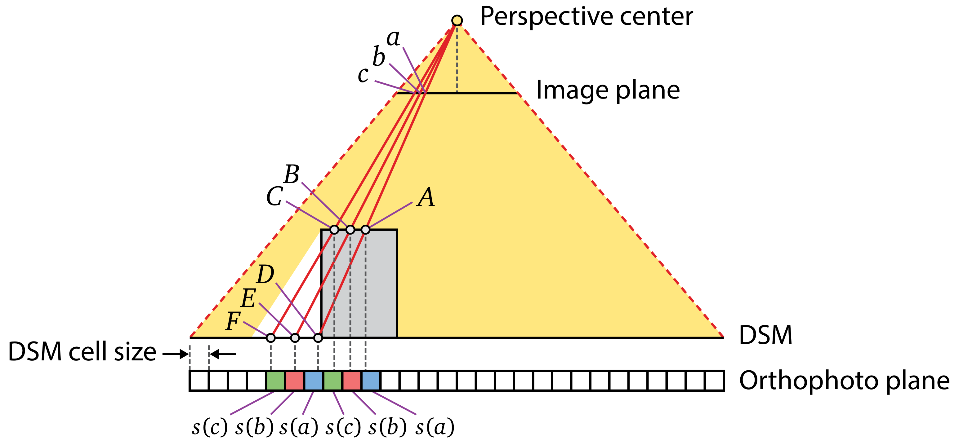
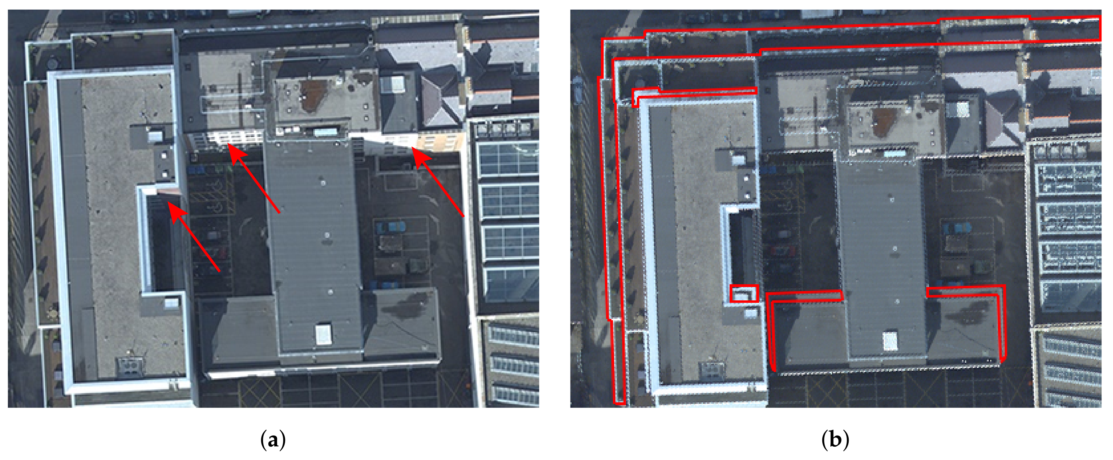
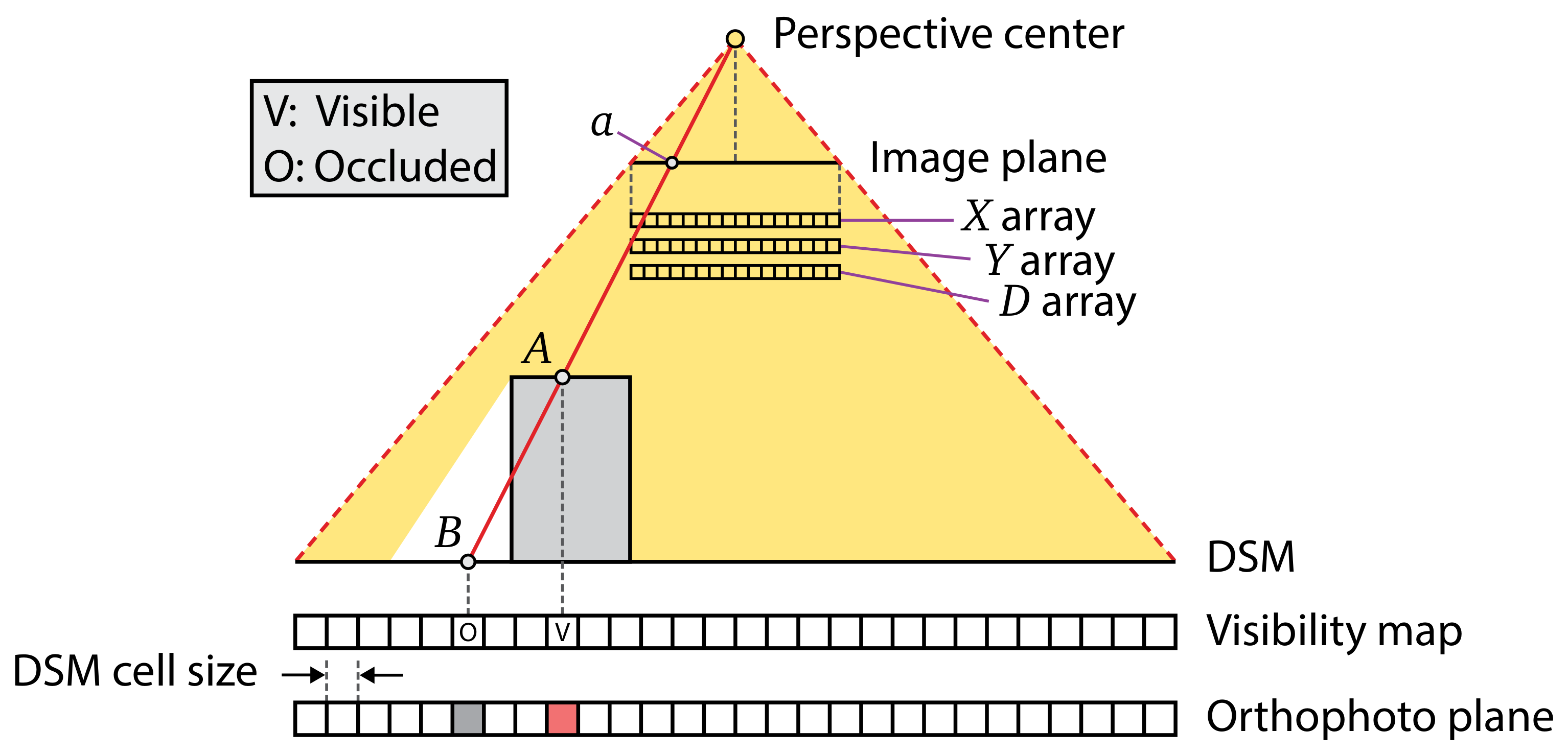
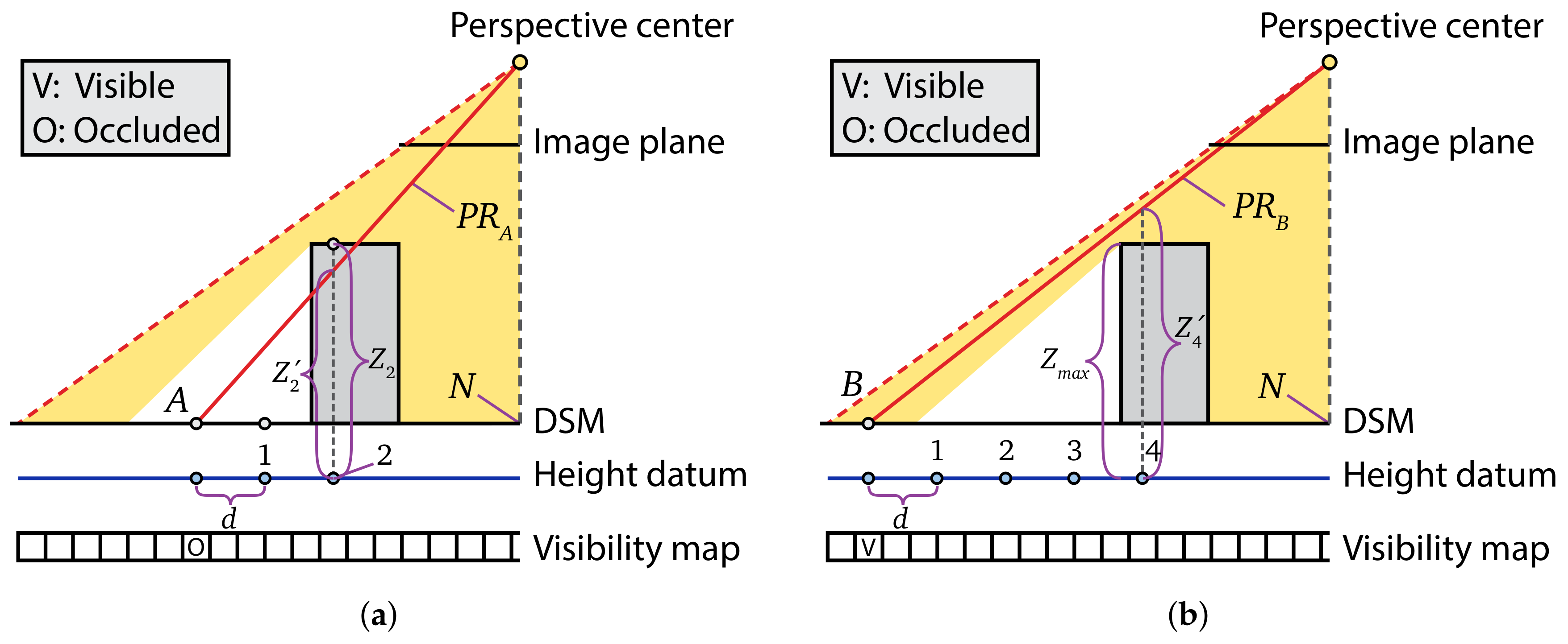
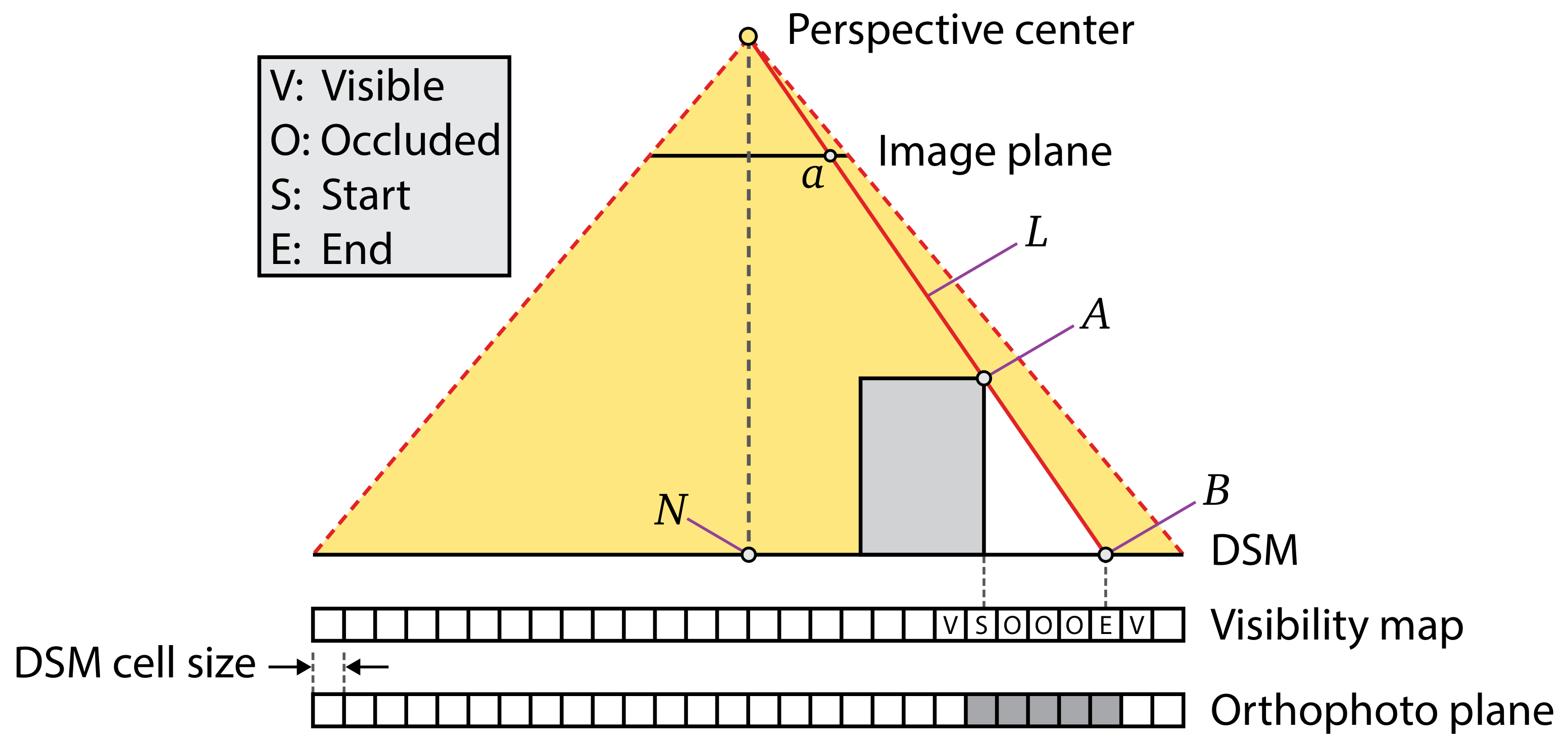
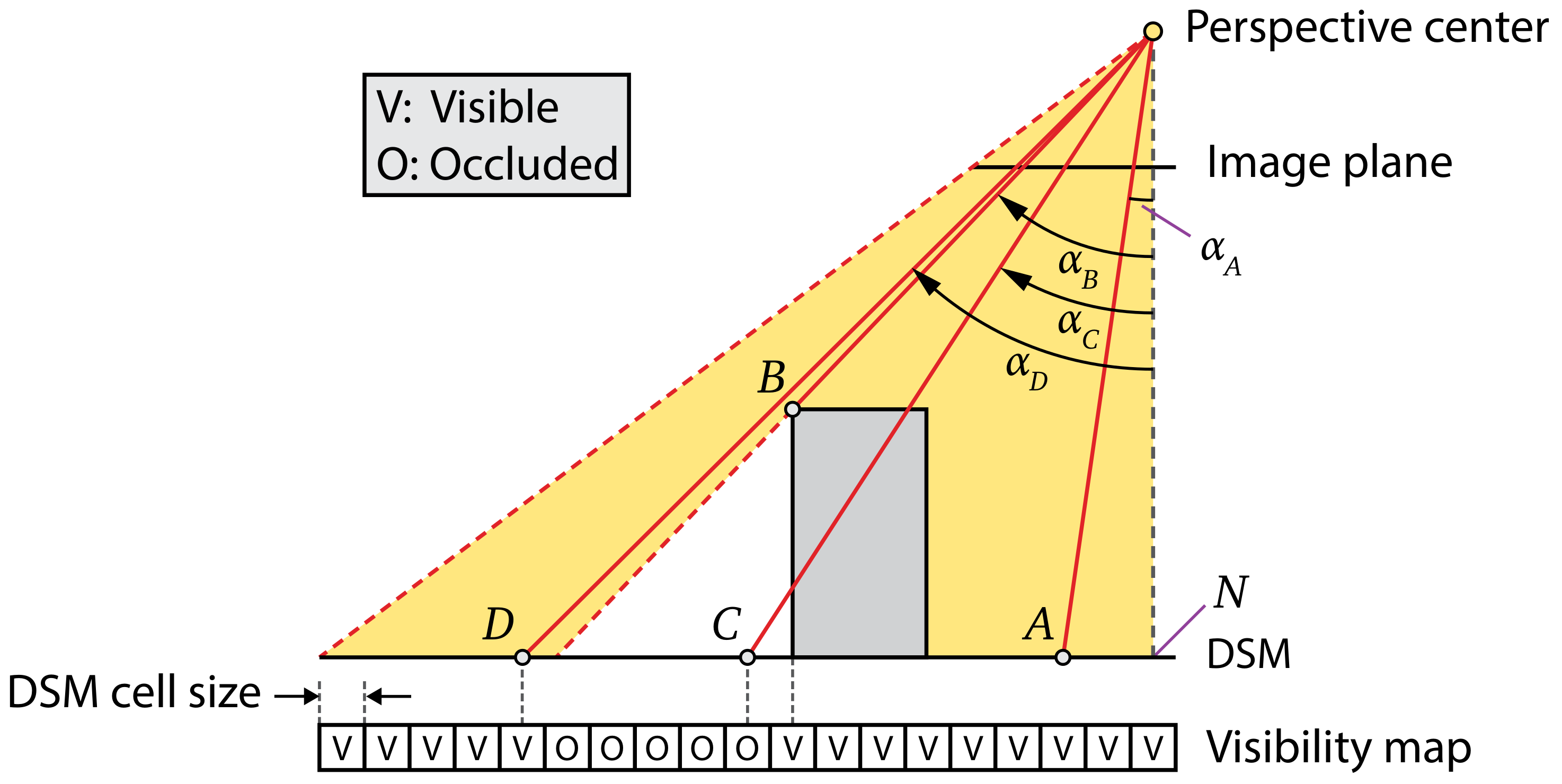
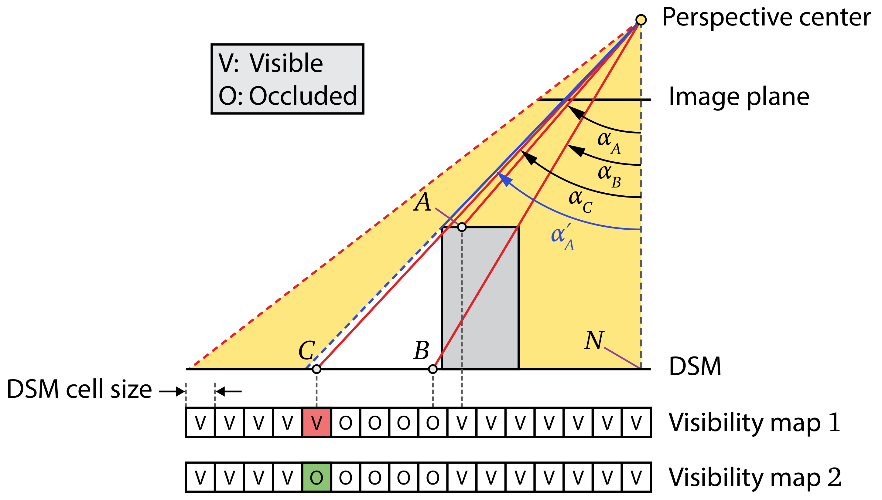
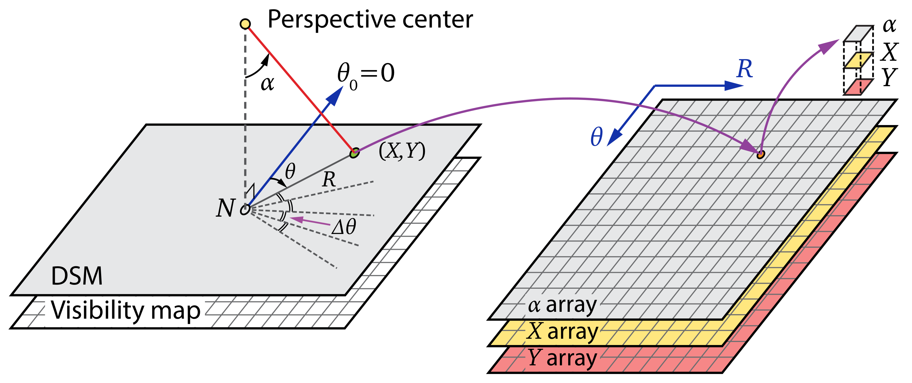
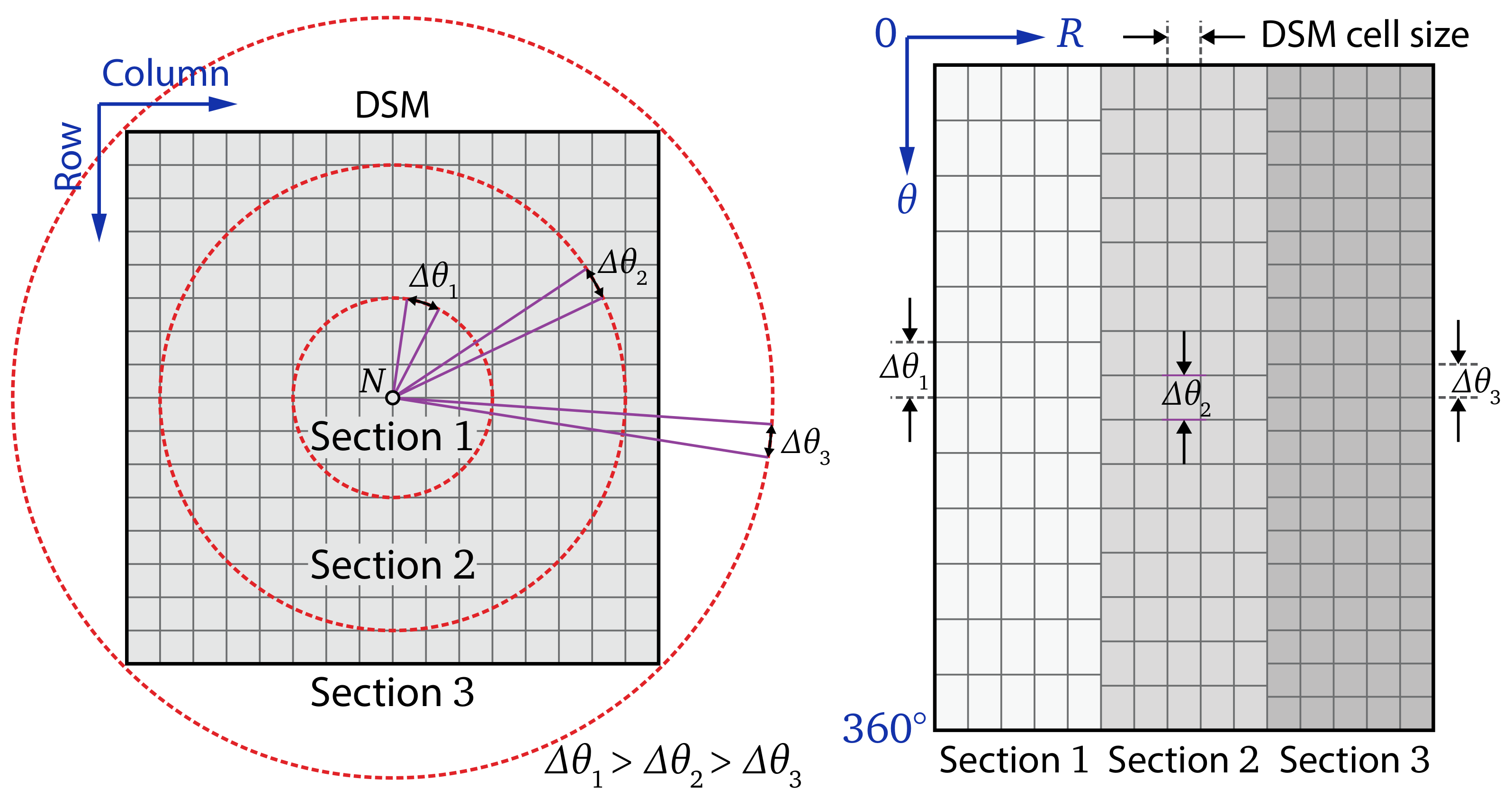
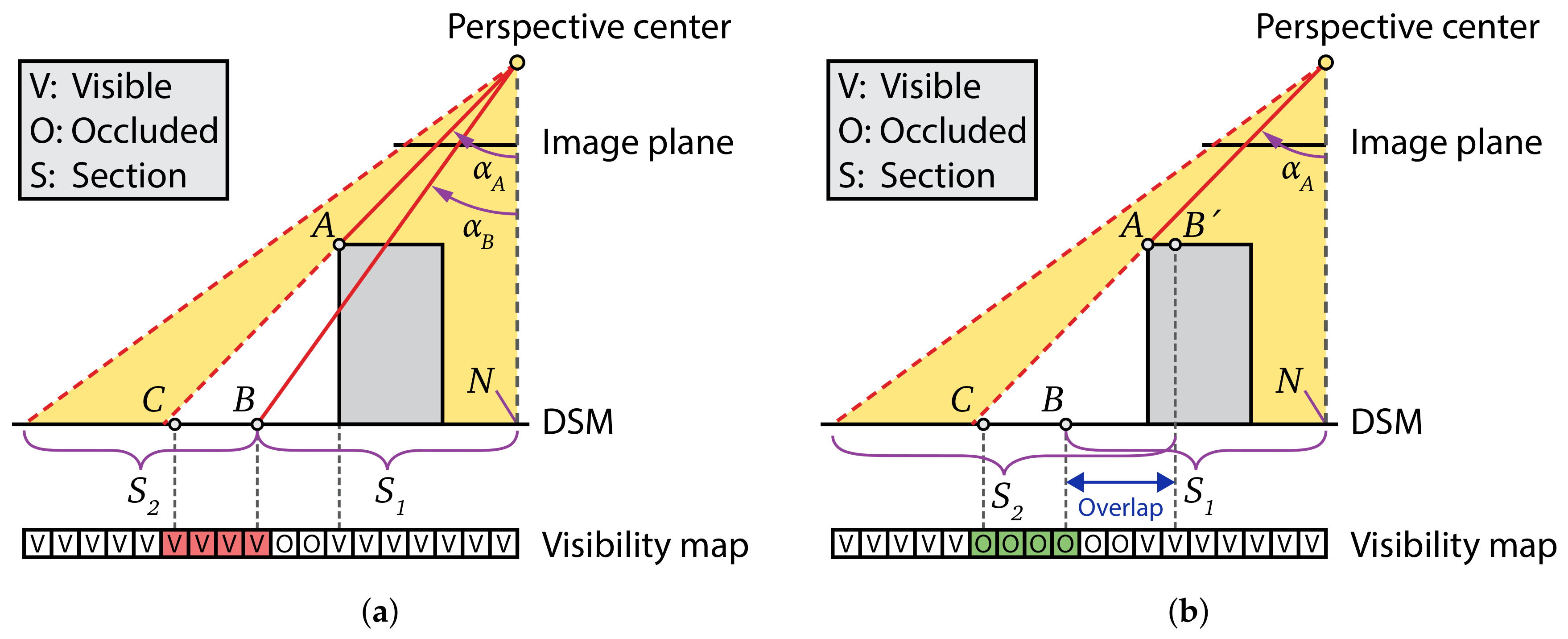
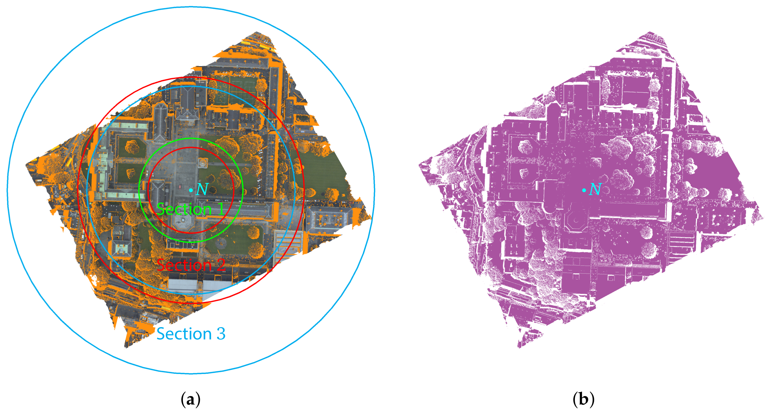
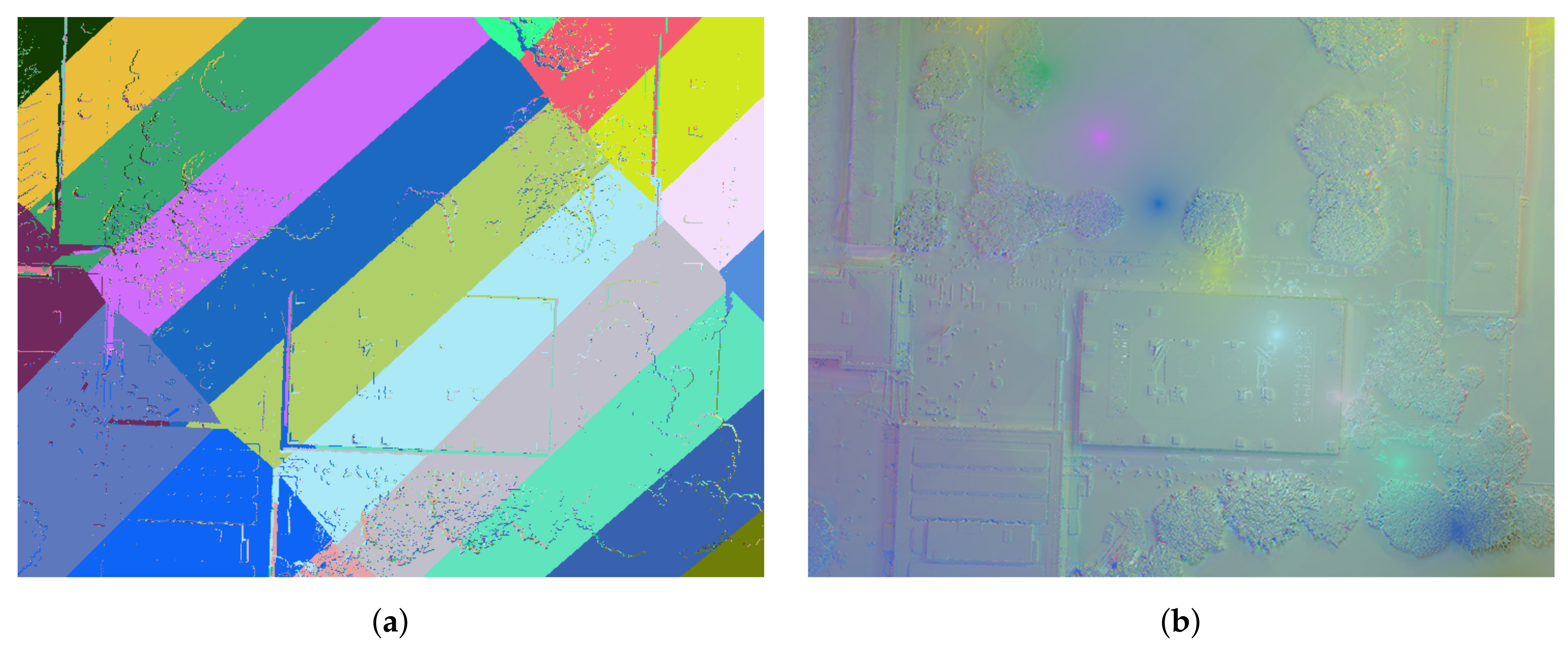
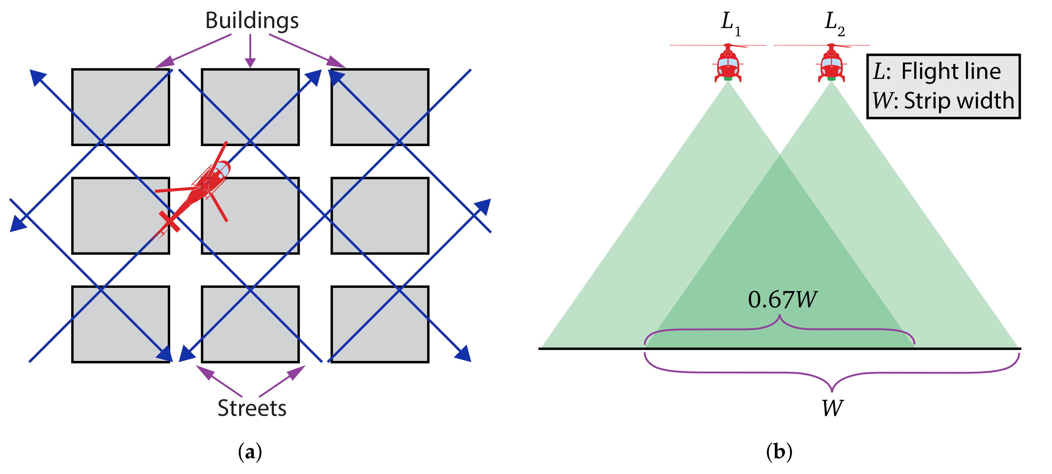
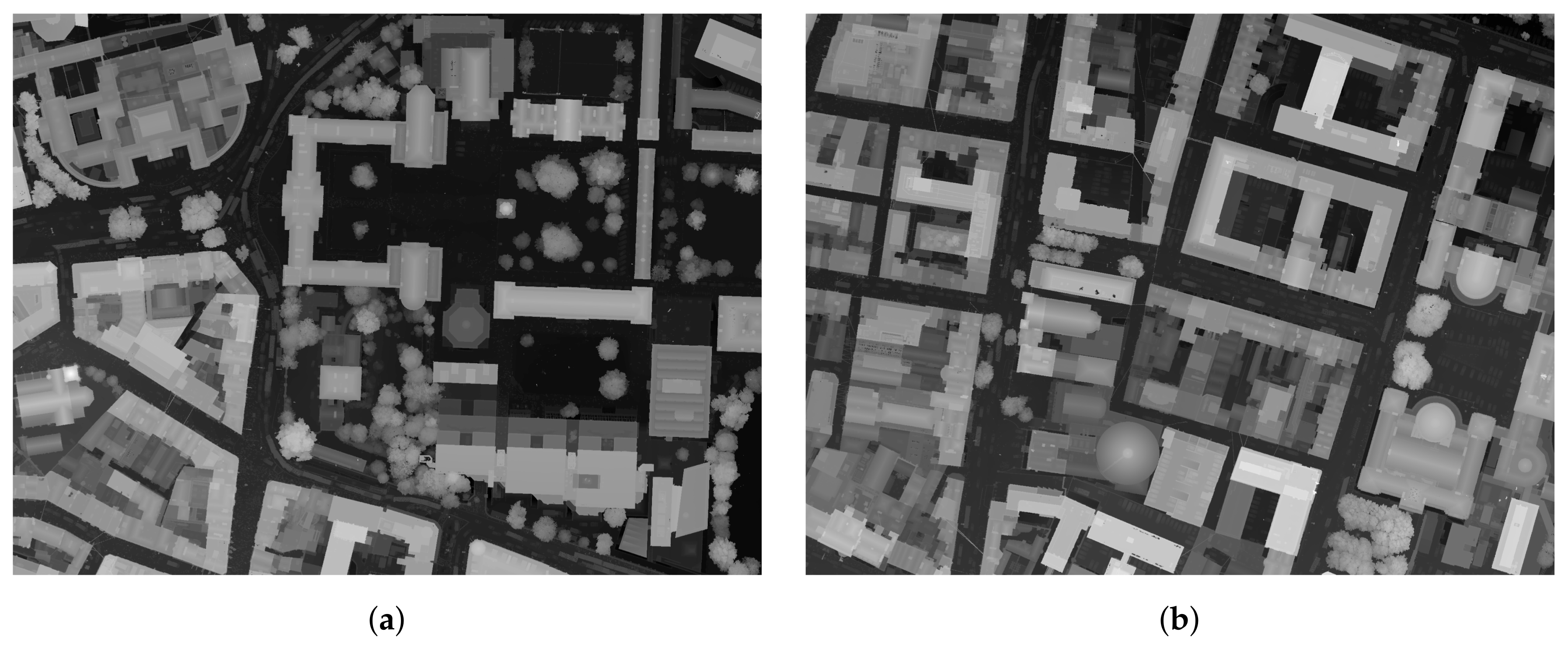
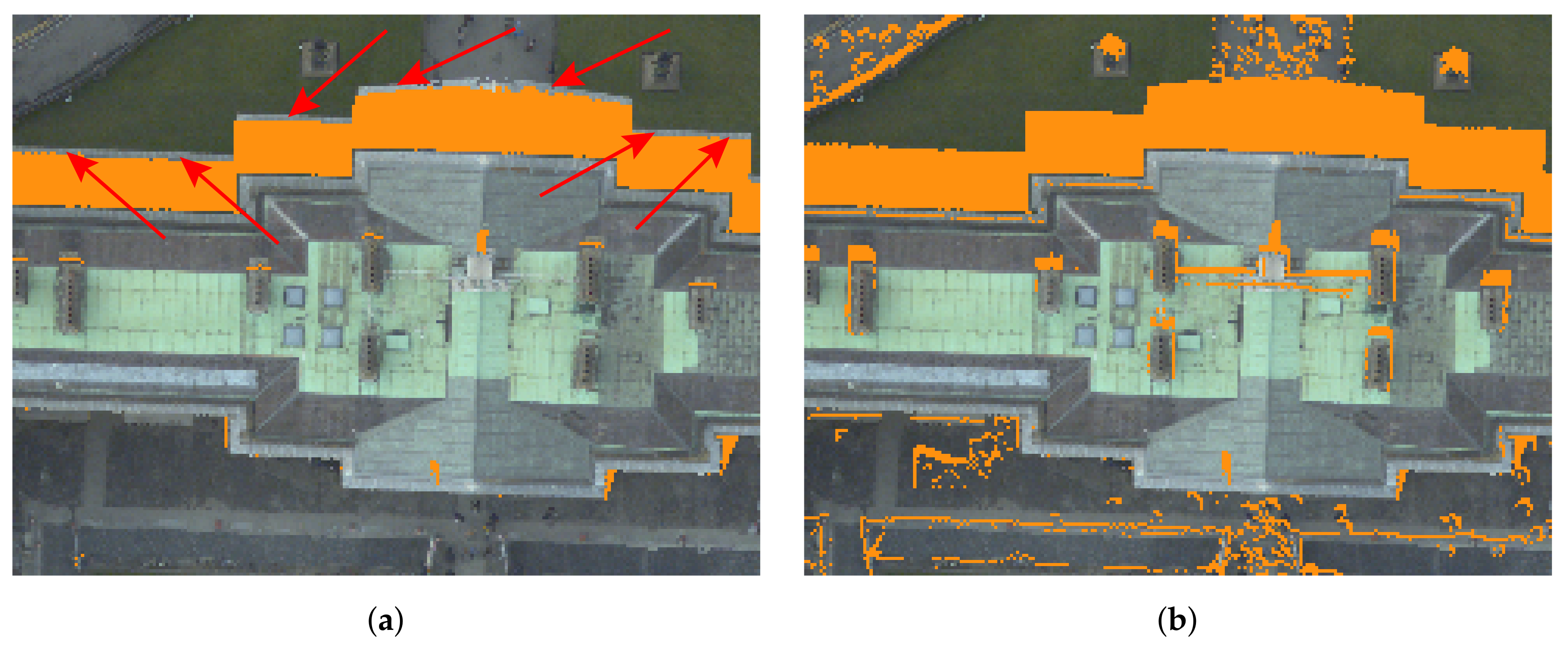
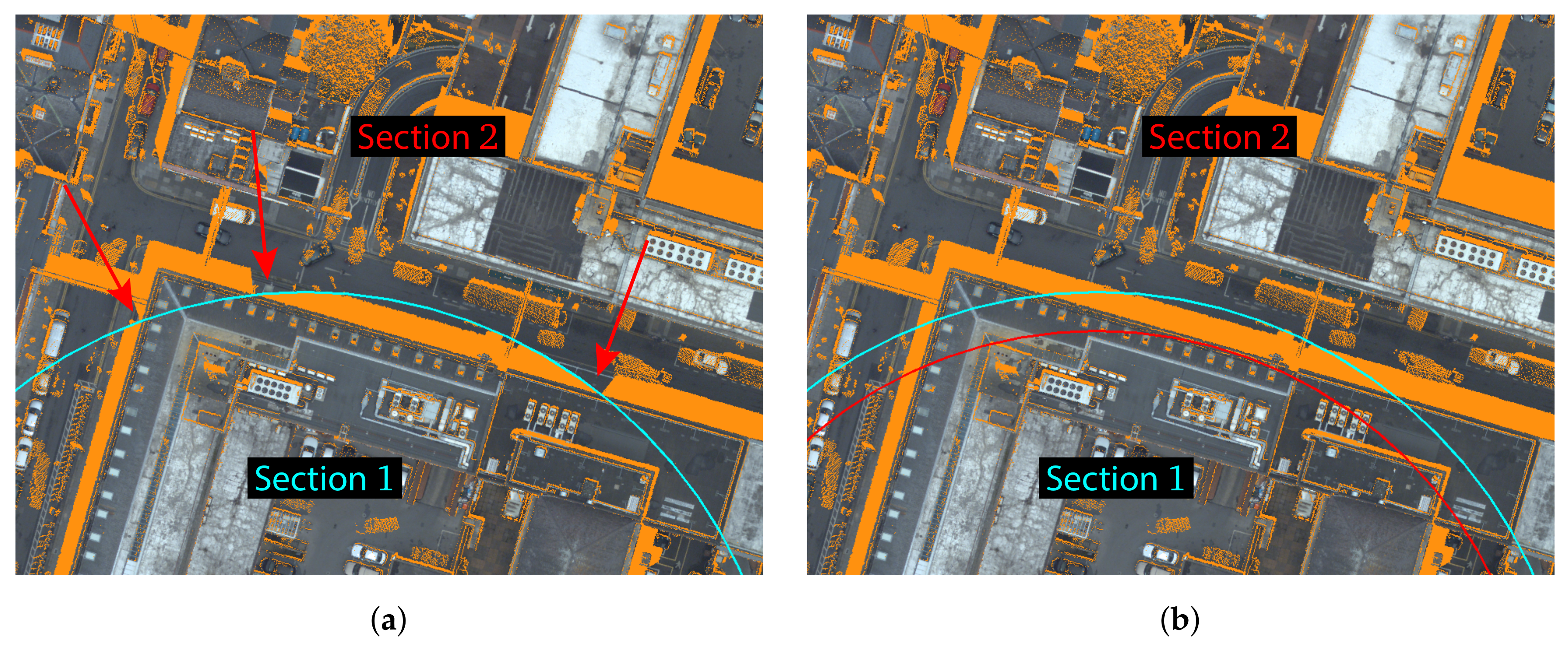
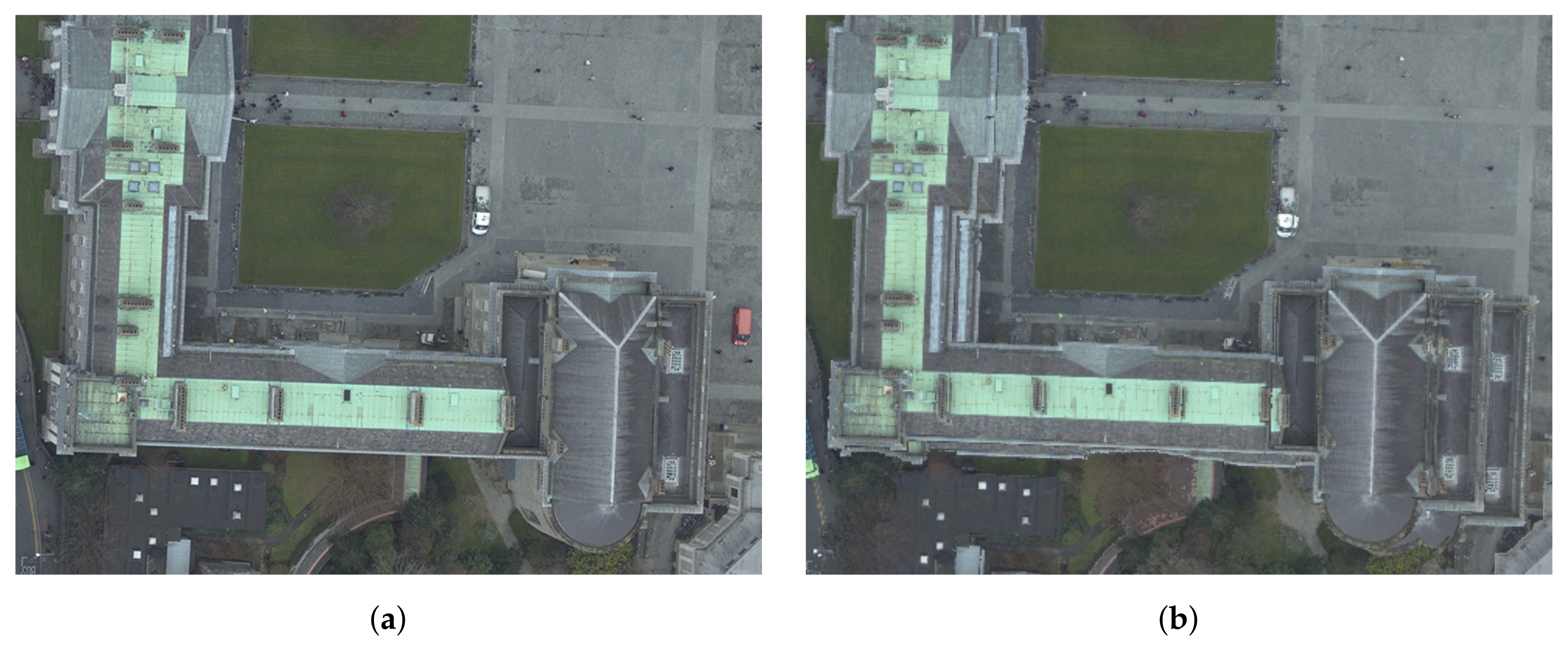
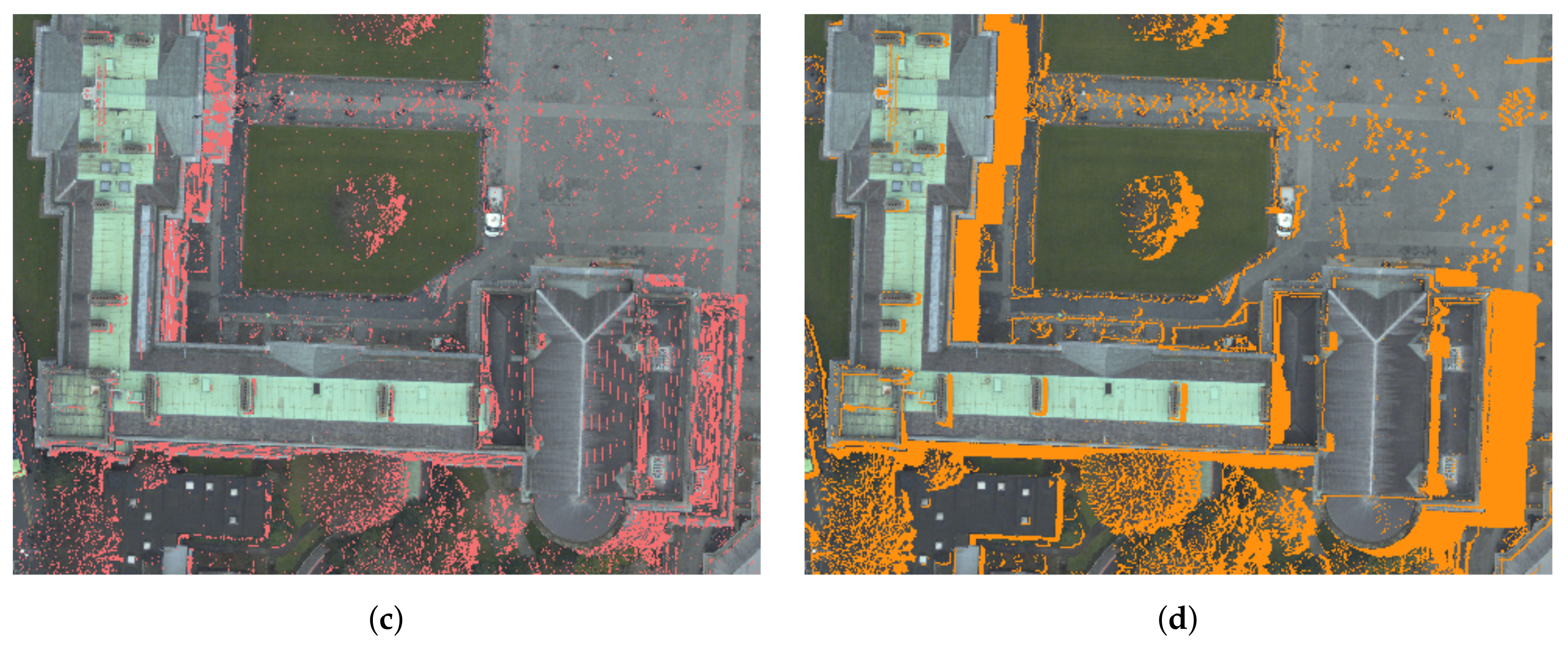
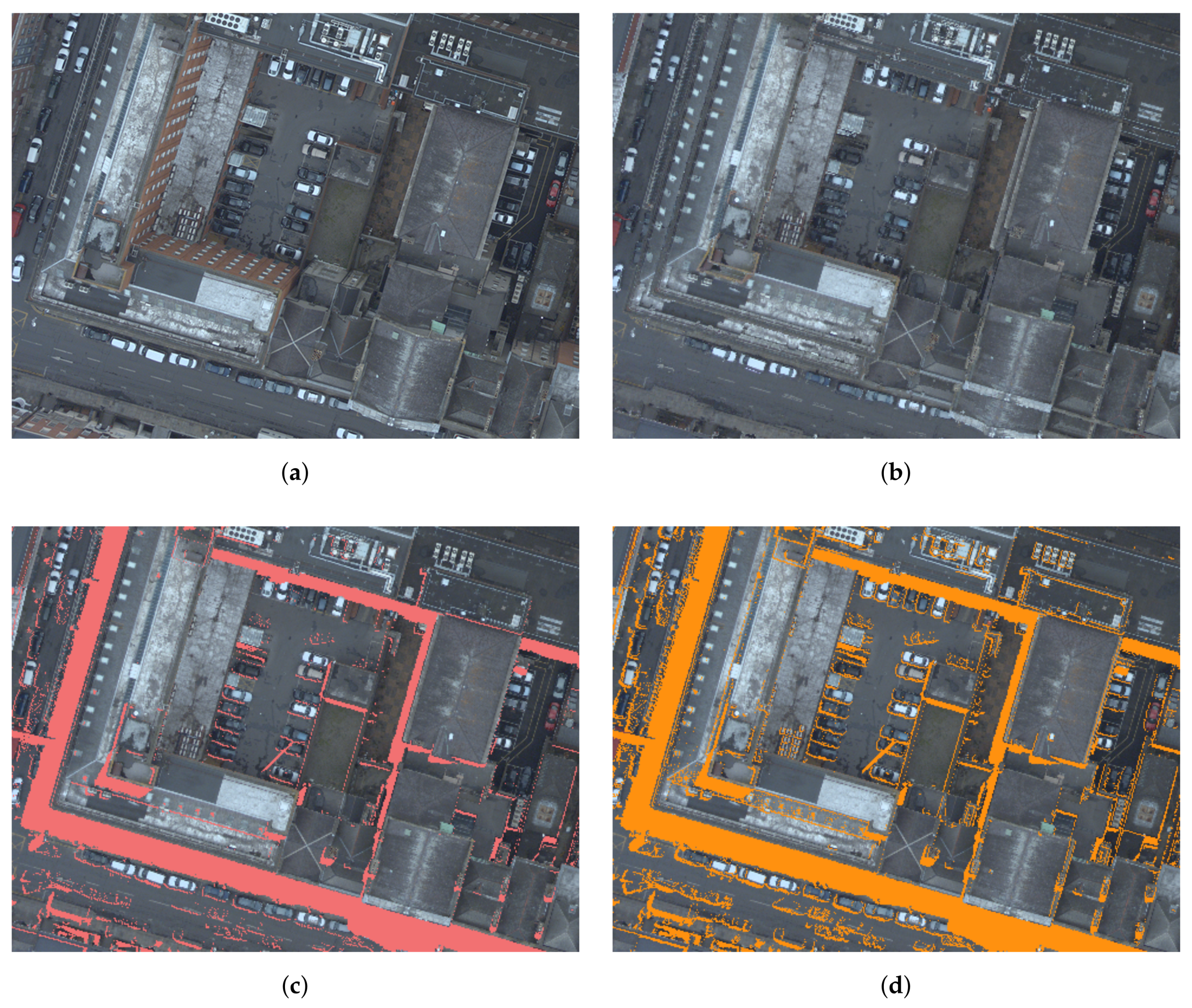
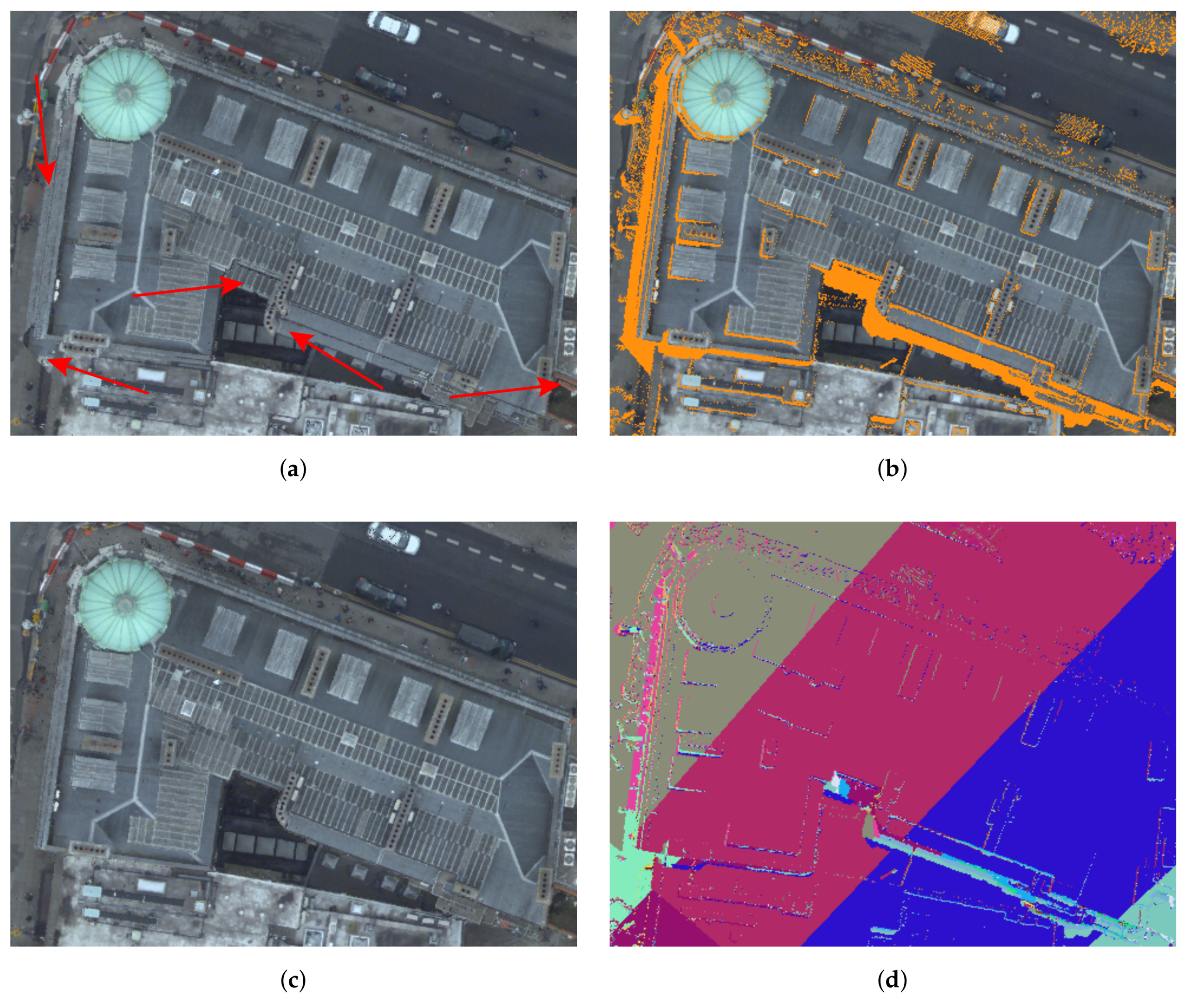
Table 1.
Specifications of the Light Detection and Ranging (LiDAR) system and the collected point data. AGL: above ground level; GNSS: Global Navigation Satellite System; IMU: inertial measurement unit.
Table 1.
Specifications of the Light Detection and Ranging (LiDAR) system and the collected point data. AGL: above ground level; GNSS: Global Navigation Satellite System; IMU: inertial measurement unit.
| Items | Values |
|---|---|
| Laser scanner system | RIEGL LMS-Q680i |
| GNSS/IMU system | POS AV 510 |
| Flying height AGL | 300 m |
| Scan angle | ( on each side) |
| Strip overlap | More than 70% |
| Swath/strip width | 350 m |
| Horizontal point density | 300 pt/m2 |
| Total no. of points | Over 1.4 billion |
Table 2.
Specifications of the utilized imaging sensor and the acquired images. GSD: ground sampling distance.
Table 2.
Specifications of the utilized imaging sensor and the acquired images. GSD: ground sampling distance.
| Items | Values |
|---|---|
| Imaging sensor | Leica RCD30 |
| Flying height AGL | 300 m |
| Frame resolution | 9000 × 6732 pixels |
| GSD | 3.4 cm |
| Along track overlap | More than 80% |
| Across track overlap | More than 70% |
| Total no. of images | 4210 |
Table 3.
Running times of the Z-buffer, height-based, and angle-based algorithms for occlusion detection using a single perspective image.
Table 3.
Running times of the Z-buffer, height-based, and angle-based algorithms for occlusion detection using a single perspective image.
| Algorithm | Running Time (mm:ss) |
|---|---|
| Angle-based | 00:07 |
| Height-based | 00:12 |
| Z-buffer | 00:04 |
Table 4.
Running time of orthophoto generation using the differential rectification technique, and true orthophoto production using the closest visible image and IDW-based spectral balancing methods.
Table 4.
Running time of orthophoto generation using the differential rectification technique, and true orthophoto production using the closest visible image and IDW-based spectral balancing methods.
| Study Area | No. of Images | Running Time (mm:ss) | ||
|---|---|---|---|---|
| Orthophoto | True Orthophoto 1 | True Orthophoto 2 | ||
| Trinity College | 98 | 03:23 | 16:17 | 31:53 |
| Dawson Street | 101 | 03:49 | 17:26 | 34:15 |
© 2018 by the authors. Licensee MDPI, Basel, Switzerland. This article is an open access article distributed under the terms and conditions of the Creative Commons Attribution (CC BY) license (http://creativecommons.org/licenses/by/4.0/).
Share and Cite
MDPI and ACS Style
Gharibi, H.; Habib, A. True Orthophoto Generation from Aerial Frame Images and LiDAR Data: An Update. Remote Sens. 2018, 10, 581. https://doi.org/10.3390/rs10040581
AMA Style
Gharibi H, Habib A. True Orthophoto Generation from Aerial Frame Images and LiDAR Data: An Update. Remote Sensing. 2018; 10(4):581. https://doi.org/10.3390/rs10040581
Chicago/Turabian StyleGharibi, Hamid, and Ayman Habib. 2018. "True Orthophoto Generation from Aerial Frame Images and LiDAR Data: An Update" Remote Sensing 10, no. 4: 581. https://doi.org/10.3390/rs10040581
Note that from the first issue of 2016, this journal uses article numbers instead of page numbers. See further details here.