Fast Approximation of Over-Determined Second-Order Linear Boundary Value Problems by Cubic and Quintic Spline Collocation


Department of Mechanical Engineering, Chair of Applied Mechanics, Technical University of Munich, Boltzmannstraße 15, 85748 Garching, Germany
*
Author to whom correspondence should be addressed.
Robotics 2020, 9(2), 48; https://doi.org/10.3390/robotics9020048
Submission received: 3 May 2020
/
Revised: 8 June 2020
/
Accepted: 23 June 2020
/
Published: 25 June 2020
Abstract
:We present an efficient and generic algorithm for approximating second-order linear boundary value problems through spline collocation. In contrast to the majority of other approaches, our algorithm is designed for over-determined problems. These typically occur in control theory, where a system, e.g., a robot, should be transferred from a certain initial state to a desired target state while respecting characteristic system dynamics. Our method uses polynomials of maximum degree three/five as base functions and generates a cubic/quintic spline, which is / continuous and satisfies the underlying ordinary differential equation at user-defined collocation sites. Moreover, the approximation is forced to fulfill an over-determined set of two-point boundary conditions, which are specified by the given control problem. The algorithm is suitable for time-critical applications, where accuracy only plays a secondary role. For consistent boundary conditions, we experimentally validate convergence towards the analytic solution, while for inconsistent boundary conditions our algorithm is still able to find a “reasonable” approximation. However, to avoid divergence, collocation sites have to be appropriately chosen. The proposed scheme is evaluated experimentally through comparison with the analytical solution of a simple test system. Furthermore, a fully documented C++ implementation with unit tests as example applications is provided.
Keywords:
cubic; quintic; spline; collocation; second-order; over-determined; boundary value problem1. Introduction
1.1. Literature Review
In almost every field of natural science and engineering we face differential equations, which are typically used for modeling dynamical systems. Especially in engineering, the more specific case of boundary value problems (BVP) is very prominent. In other words, one often searches for the behavior of the investigated system between some kind of fixed, i.e., known, spatial or temporal boundaries. One can try to derive the analytical solution to the problem, however for complex systems this can be difficult or even impossible. In such cases, it can be sufficient to approximate the solution for which a variety of techniques exists.
Methods based on finite differences approximate the derivatives by difference quotients to obtain a system of equations which depends only on the primal function. This allows a solution to be found by formulating a linear system of (algebraic) equations representing the transformed system at certain grid points. In contrast, shooting methods aim at the iterative solution of an equivalent initial value problem (IVP), which is typically easier to handle than the original BVP. While for single shooting the IVP is evaluated over the complete time interval, multiple shooting considers a partitioned time domain. Another technique is given by the finite element approach, which is mainly used for partial differential equations (PDE) as they occur, for example, in structural-, thermo-, and fluid dynamics. Typically finite element methods are based on a weak formulation of the residual and on splitting the considered domain into elements on which the local base functions to approximate the solution are defined. Although designed for PDEs, they can be applied to the simpler case of ordinary differential equations (ODE), which are the focus of this contribution (see, for example, [1]). A variety of other techniques exist. However, these three groups appear to be used the most in the field of engineering.
In the following, we approximate the solution through spline collocation using piecewise polynomial trial functions, which is a well-known technique to solve BVPs, see, for example, [2,3,4]. Over the past decades, various algorithms emerged, which can be classified into two types. The first type, also known as smoothest spline collocation (or just spline collocation as in [5]), aims at matching the differential equation at one collocation site per spline segment, which is typically a knot or the mid-point of the segment, while simultaneously forcing the spline to have maximum smoothness, i.e., highest possible continuity [5]. The second type, in [5] called Gaussian collocation, removes the constraints on higher order continuity and instead uses more collocation sites, which are typically chosen to be the Gaussian points of each segment. This class, which is also called orthogonal spline collocation [6], originates from [3] and aims at maximizing the order of convergence. In order to also provide a competitive convergence for the first type of methods, special variants for quadratic and quintic spline collocation have been proposed in [7] and [8], respectively. Optimal methods for quadratic and cubic splines on non-uniform grids, i.e., for an inhomogeneous segmentation of the spline, have been presented in [5].
Note that in addition to general purpose codes, such as COLSYS (FORTRAN) for non-linear mixed-order systems of multi-point boundary value ODEs [9], highly specialized algorithms, which aim at obtaining the best possible approximation for certain use cases, have also been published. Recent examples are methods for integro-differential equations [10] or fractional differential equations [11], which occur in certain material models exhibiting memory effects. Along with ODEs, various kinds of (multi-variable) PDEs have been investigated. See [6] for a survey on corresponding Gaussian collocation methods. Note that, for PDEs, the time domain is typically discretized using finite differences, e.g., by the Crank–Nicholson approach as used in [6], or the second-order backward difference in [10], while spline collocation is used for approximating the spacial variables. Lastly, methods for differential algebraic equations (DAE) have also been developed, e.g., the COLSYS extension COLDAE [12] for semi-explicit DAEs of index 2 and fully implicit DAEs of index 1.
In our opinion, despite the variety of techniques, there is still a lack of simple methods prioritizing execution time over approximation quality, which is essential for time critical control applications. The aim of this contribution is to provide an algorithm satisfying these needs while focusing on the special case of second-order linear ODEs, which are very common for dynamic systems. Moreover, we focus on over-determined BVPs, i.e., where more boundary conditions (BC) are given than necessary. This may at first seem to be a restriction of our algorithm since it needs more information than other implementations; however, it allows us to also consider inconsistent BVPs, i.e., the case where no exact solution to the problem exists.
1.2. Motivation
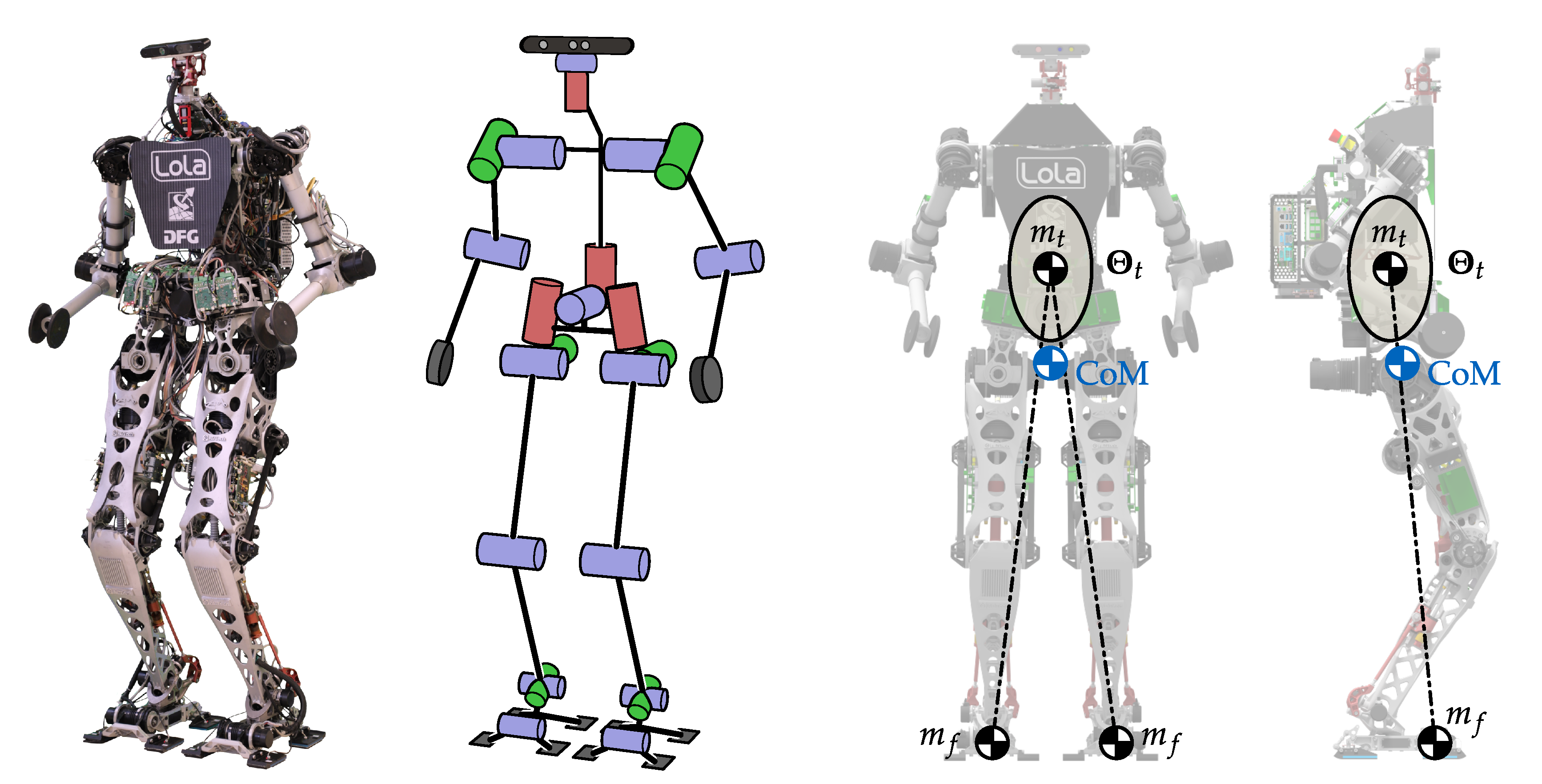
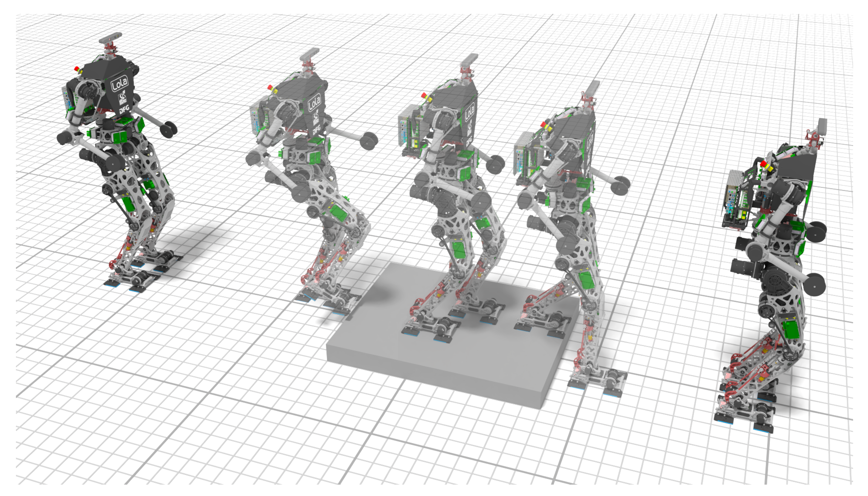
It might appear strange to search for an approximation of something that actually does not exist. However, we face exactly this situation during walking pattern generation for our humanoid robot LOLA, cf. Figure 1 left. In particular, we use a simplified model of the robot’s multi-body dynamics, cf. Figure 1 right, to plan the center of mass (CoM) motion over a certain time horizon. The planned CoM motion resembles the dynamics of the model, which can be formulated as second-order linear ODE, and is constrained to certain values on position-, velocity- and acceleration-level at the boundaries of the planning horizon. This leads to an overdetermined BVP of the type investigated in this contribution. The BCs at the beginning reflect the current state of the robot, e.g., the standing pose in front of a platform, while the BCs at the end represent the target state, e.g., the standing pose on the other side of the obstacle, cf. Figure 2. For a seamless motion of the robot it is crucial to guarantee the satisfaction of the BCs, i.e., a perfect match of the boundary states. In contrast, it is sufficient to approximate the dynamics of the underlying ODE since it is derived from a simplified model which is an approximation in itself. This is the key idea behind the formulation of an over-determined BVP, which may thus not have a proper “real” solution. To the authors knowledge, all comparable algorithms assume that a solution of the BVP exists, while most of them also require it to be unique and “sufficiently” smooth.
Explaining the technical details of the walking pattern generation framework of LOLA goes beyond the scope of this paper. Instead, the interested reader is referred to [13], in which the application of the proposed algorithm is presented. The publication [13] comes with an accompanying video, see [14], which visualizes the sequential steps of the walking pattern generation pipeline of LOLA. The simulations and experiments presented in the video show the successful application of our algorithm. In the following, we do not further restrict ourselves to this special application. Since the proposed algorithm is generic, we derive it in the most general way since it may be useful also for different applications in robotics.
1.3. Additional Remarks
Our method can be seen as smoothest spline collocation, i.e., it belongs to the “first” type as classified in Section 1.1. We do not apply special techniques to increase the order of convergence, but instead adhere to its basic form. This leads to a much simpler derivation and implementation. In addition it makes the algorithm faster by sacrificing approximation quality. This complies with the needs of our target application as explained in Section 1.2. We emphasize that our focus lies on simplicity, robustness, and efficiency. Thus we will not search for a mathematical formulation of the convergence order. Instead, the algorithm is evaluated mainly through experiments, where runtime performance is our primary concern.
As summarized in Section 1.1, there exist numerous methods for solving linear BVPs or spline interpolation/collocation in general. For most approaches, solving a large-sparse or small-dense linear system of equations (LSE) represents the main workload. To overcome this bottleneck, parallelized algorithms have been developed, which typically exploit the special structure of the involved matrices, e.g., the scheme proposed in [15] for staircase matrix structures. Although we aim at efficiency, we do not consider explicit parallelization as acceleration technique. This is because our algorithm is designed for embedded systems which typically feature only few physical CPU cores running also other time-critical tasks. Moreover, the use of GPUs, e.g., through CUDA or OPENCL, is often not feasible since the CPU–GPU interface lacks capabilities for hard real-time requirements. Finally, dedicated to our target application, we only consider (comparatively) small problems with runtimes . For such systems the performance boost obtained through parallelization is likely to be canceled out by the synchronization overhead. Nevertheless, our algorithm may also be used for large scale problems. In this case an “off the shelf” parallel solver for dense LSEs may be used, cf. [16]. However, one should keep in mind that by using an iterative scheme execution time is not deterministic anymore, and, even worse, the solver might not converge. As an alternative, there exists an efficient way for the parallel solution of decoupled, multi-dimensional BVPs, which takes advantage of intermediate results, see Appendix C for details.
2. Materials and Methods
In the following, two versions of our algorithm are presented: one using a cubic spline and the other using a quintic spline for approximating the BVP. As the derivations and resulting algorithms are similar, we show the connecting links by presenting both methods in parallel. The version based on cubic splines is naturally simpler, although, using quintic splines leads to a smoother approximation. Indeed it is - instead of -continuous, which can be preferable for some use cases. Moreover, quintic splines allow us to directly preset first and second-order derivatives at both boundaries, which otherwise requires the introduction of virtual control points and in turn can lead to poor results, as discussed in Section 3. Although deriving the proposed collocation algorithm for quintic splines is more advanced than its cubic counterpart, overall performance is superior, because the same approximation quality can be obtained with less collocation sites and hence with less computational effort as shown in Section 3. However, this requires the underlying ODE to be sufficiently smooth. Note that, in contrast to our intention, most other investigations choose quintic splines for approximating fourth-order ODEs, e.g., in [8,10,11,17] (similar to choosing cubic splines for second-order ODEs).
We highlight that the proposed method is not only inspired by, but is also heavily based on the interpolation and collocation algorithms presented in [18,19], respectively. The main contribution of this paper is the combination, extension and runtime optimization of those methods. Moreover, we provide a detailed and self-contained derivation together with a fully documented open-source C++ reference implementation.
Having a background in mechanical engineering, the authors intention is to present a simple and self-contained derivation of the proposed algorithm, which can be easily understood, implemented, and extended by readers also lacking a dedicated mathematical background.
2.1. Problem Statement
Consider the second-order linear time-variant ODE
where and denote the first and second derivative of the unknown function with respect to time t, i.e.,
Note that t does not have to represent time. However, this synonym is used in the following due to the typical appearance of (1) in dynamical systems. The coefficients , , , and the right-hand side are arbitrary, in general nonlinear, but known functions of t. Let system (1) be constrained by the BCs
where and define the considered time interval and , , , , , are user-defined constants. Then system (1) together with the BCs (2) represents the second-order linear two-point BVP for which an approximation is to be found. Note that (2) considers Dirichlet, Neumann, and second-order BCs independently of each other. In contrast, various other algorithms assume Robin BCs, i.e., a linear combination of Dirichlet and Neumann BCs, which is not equivalent to our approach. Due to (2), the BVP is over-determined and the existence of a solution depends on the consistency of the BCs with the ODE.
In the following, we investigate the approximation of through spline collocation, i.e., we generate a spline which satisfies the underlying ODE (1) at a user-defined set of distinct collocation sites , numbered in increasing order, which lie within the considered interval , i.e.,
Moreover, is forced to fulfill the BCs (2) at and , i.e.,
Here we use to denote the approximating spline while the exact solution is represented by . For clarity, we also use different denominations for and by using the terms collocation sites and collocation points, respectively. While are user-defined parameters, describe the solution to be found.
Since the proposed collocation algorithm is strongly related to the interpolation of cubic/quintic splines, which may not be common to some readers, spline interpolation is recapitulated in Section 2.3. Then, the proposed collocation method is derived in Section 2.7. Moreover, we reuse core elements of the interpolation algorithm during collocation, thus we cannot omit its derivation.
2.2. Spline Parametrization
Before diving into the derivation of algorithms, one first has to decide which spline representation to use. In the literature, formulations such as basis splines (B-splines) are common, since they feature inherent continuity and local control, which typically leads to banded systems [20]. In general, B-splines do not pass through their control points, which seems to make interpolation difficult at first sight; however, efficient algorithms for interpolation and collocation exist, see, for example, [21]. In [20], it has been shown that B-splines might not be as stable and efficient as other representations, namely monomial and Hermite type bases, especially when it comes to implementation. In particular, monomial bases have been recommended due to their superior condition, and thus lower roundoff errors. For all three forms, B-spline, Hermite type, and monomial, the core operation during Gaussian collocation is typically the solution of an almost block diagonal (ABD) linear system of equations [6,21]. A generic solver for these type of systems is SOLVEBLOK [22], while the special structure occurring for monomial bases is exploited by ABDPACK [23] with increased speed and lower memory consumption. Unfortunately, for smoothest spline collocation as presented in the following, the corresponding collocation matrix is dense, thus we cannot apply these algorithms. However, when compared to Gaussian collocation, the count of collocation sites and thus the dimension of the corresponding LSE is much smaller, which can lead to comparable performance.
Despite the popularity of B-splines, we use the so-called piecewise polynomial (PP) form [21], which describes the spline through the coefficients of interconnected, but independently defined, polynomial segments. We use a special type of monomial bases, namely the canonical form of the polynomials, which may not be as efficient as the choice in [20]; however, it makes our algorithm much simpler. By using this formulation, continuity between the spline segments needs to be explicitly established. The evaluation of the resulting spline, however, boils down to the evaluation of a single polynomial belonging to the corresponding segment, which is in general much quicker than evaluating the equivalent B-spline form. The evaluation of B-splines of degree p with the well-known de Boor’s algorithm [24] takes operations [25]. There are optimized versions of it as proposed in [25,26]; however, these are numerically less stable [27]. In contrast, evaluating a polynomial of degree p with Horner’s method [28] takes only , i.e., , operations [29]. This is essential for time-critical applications, where the resulting spline has to be evaluated as quickly as possible. Note that we are free to construct the spline in B-spline formulation and convert it to the corresponding PP form in a post-processing step, see [21]. However, this introduces an additional (expensive) step which we try to avoid since, in our case, not only the evaluation but also the construction of the spline is time critical.
Let the spline be defined as
where represents the i-th of the spline segments parametrized by the normalized interpolation parameter . We call and the global and local interpolation parameters, respectively, for which we choose the linear mapping
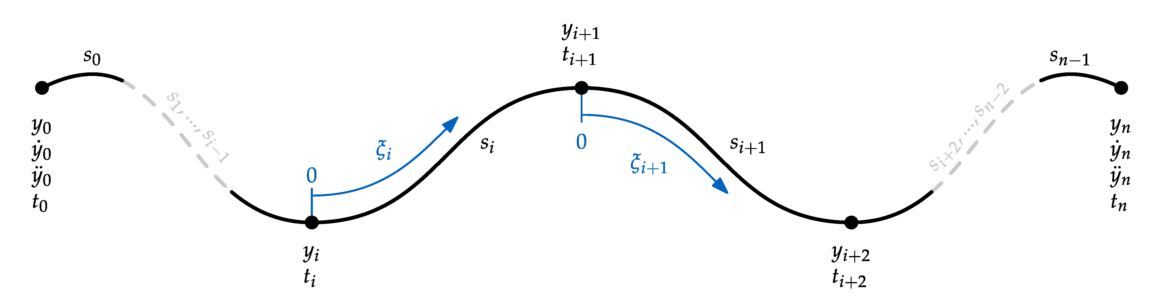
with as the duration of the i-th segment and its reciprocal . The partitioning of the spline into n segments is visualized in Figure 3. In the following, we predominantly derive expressions in local segment space, i.e., with respect to , since this makes the notation clearer, especially in Section 2.7. Note that, in contrast to some other approaches, we do not require homogeneous partitioning, thus the segmentation can be chosen arbitrarily as long as spline knots do not coincide. However, in Section 2.3, we show that for best numerical stability uniform partitioning should be used.
In the case of cubic splines (left subscript C), each segment represents a polynomial of degree three,
where , , , and are its constant coefficients. The first two derivatives of with respect to t are obtained by applying the chain rule:
For quintic splines (left subscript Q), each segment represents a polynomial of degree five,
where , , , , , and are its constant coefficients. As in the cubic case, we obtain the first four derivatives of with respect to t through the chain rule:
2.3. Spline Interpolation: Preliminaries
In the following, we recall how a given set of data points with can be interpolated with a or smooth cubic or quintic spline, respectively. The derivation explicitly uses the PP form of the spline and leads to the same algorithm as presented in [18], except for slight modifications in notation. Note that [18] only deals with quintic splines. However, the method for cubic segments presented in this paper is a simplified version of the same scheme. Moreover, the derivation is investigated in more detail than it is in [18]. Readers not interested in these details are referred to Algorithm 1 which summarizes the results of this section.
In contrast to [18], we only consider the case of predefined first- and second-order derivatives at the boundaries of the quintic spline, i.e., we assume , , , and to be given (as indicated in Figure 3). For the cubic counterpart, we lose two degrees of freedom, allowing us to predefine only two constraints out of . For the remainder of this section, we restrict ourselves to the case of predefined second-order time derivatives and as this allows an efficient algorithm similar to the one presented for quintic splines. Note that this choice includes the common case of natural cubic splines, i.e., . For cubic splines, we postpone the enforcement of the remaining boundary conditions, i.e., and , to the end of Section 2.7.
In the following, we only consider distinct and ascending interpolation sites, i.e., for .
2.4. Cubic Spline Interpolation: Derivation
Since our goal is a spline which passes through the given data points , we enforce the interpolation constraints
Furthermore, we aim at continuity, thus we further require that
Inserting (7) and (9) into (15) and in the second row of (16) allows us to reformulate the spline coefficients as
where for are the unknowns which have to be computed using the remaining equations given by the first row of (16). For this purpose, we expand the first row of (16) with (8) and insert , , and from (17) to obtain
which holds for . This equation can be considered as defining intermediate unknowns and can be written as LSE of the form
with and , given by
and their elements
Herein , , and represent the lower diagonal, diagonal, and upper diagonal elements of , respectively. Note that only depends on the choice of , thus it can be reused in case we need to perform further interpolations with the same segmentation . While represents the interpolation sites , the interpolation points are encoded in . The additional term incorporates the BCs such that we can write the system in the neat form of (20). From the solution we can directly obtain the unknowns which in turn can be used together with the data points and BCs to compute the segment coefficients (17) such that the spline is fully defined. Note that is symmetric, i.e., ; however, we do not make use of this property.
Although one can compute from (19) using an arbitrary solver for linear systems of equations, there is a more efficient way for doing so: since is tridiagonal, we can solve (19) with the Thomas algorithm [30,31]. Derived from an decomposition of , one performs a recursive forward elimination
followed by a backward substitution
Computing out of and thus boils down to operations. Note that in contrast to [31] where in our case , thus n changes to for computing the count of operations in total [31]. Since is symmetric and positive definite, one may think of using an algorithm based on Cholesky factorization instead of decomposition, as this has proven to be approximately twice as efficient where applicable. However, this rule of thumb seems to be no longer valid for the special case of tridiagonal matrices: the Cholesky factorization in [32], where the computation of the lower diagonal matrix L exploits the special structure and the diagonal matrix is used to avoid evaluating expensive square roots, leads to operations in total.
The numerical stability of cubic spline interpolation is shown in Appendix A.1.
2.5. Quintic Spline Interpolation: Derivation
As previously mentioned, the following is a detailed version of the derivation given in [18]. Just as in the cubic case, our task is to pass through the given data points , thus we enforce the interpolation constraints
We use the additional degrees of freedom to enforce not only , but instead continuity with
Inserting (10), (11), and (12) into (28) and into the first two rows of (29) allows us to reformulate the spline coefficients to
where and for are the unknowns which we still have to determine using the remaining equations given by the last two rows of (29). In particular, we expand the fourth row of (29) with (14) and insert , , and from (30) to obtain
In the same manner, we expand the third row of (29) with (13) and insert , , and from (30) which leads to
Both (31) and (32) hold for which allows casting them in the form of
with and , given by
and their block components
Just as in the cubic case, , , and represent the lower diagonal, diagonal, and upper diagonal blocks of , respectively. As suggested in [18], the additional parameter in the definitions (35)–(38) is chosen as
From an analytical point of view, has no influence on the solution (at least if ). However, it improves numerical stability which is verified in Appendix A.2.
As for the cubic spline is symmetric and only depends on the choice of , while the interpolation points are contained in . As before, the additional term incorporates the BCs such that we can write the system in the form of (34). In contrast to the cubic case, the solution represents not only , but also , which is now additionally required to compute the segment coefficients from (30).
Since is block-tridiagonal, we can again solve (33) efficiently with the generalization of the Thomas algorithm to block-tridiagonal matrices [31]. Based on an decomposition of , we first run a recursive forward elimination
followed by a backward substitution
Computing out of and requires at a maximum operations. Again [31] uses while in our case holds, thus n changes to for computing the count of operations in total [31]. For this upper bound, explicit computation of the inverse of and by Gaussian elimination is assumed, which in practice should be avoided by solving a LSE instead [31]. Thus, a corresponding implementation can be expected to require even less operations.
In Appendix A.2, the interested reader can find considerations on the numerical stability of quintic spline interpolation.
2.6. Algorithm for Cubic/Quintic Spline Interpolation
Since the presented derivation is rather lengthy, the key steps for interpolating cubic/quintic splines following the proposed method are summarized in Algorithm 1.
| Algorithm 1: Cubic/Quintic Spline Interpolation. |
 |
For details on convergence order and approximation error of quintic spline interpolation, the interested reader is referred to [18] where these issues have been experimentally investigated for various examples.
2.7. Spline Collocation: Derivation
The following is based on the collocation algorithm presented in [19,33]. However, we extend the method from cubic to quintic splines. Moreover, we do not use natural splines, but instead integrate the boundary conditions directly into the scheme. Lastly, in contrast to [19,33], we do not need to modify the right-hand side of (1), thus leading to a “true” collocation of the ODE for all collocation sites, which are chosen to be the interior spline knots. As runtime performance is of the highest priority for our application, we choose smoothest spline collocation. This minimizes the count of (expensive) collocation sites, thus reduces the count of equations to solve, and instead uses the available degrees of freedom to force (cubic spline) or (quintic spline) continuity. Moreover, in our application, is used as input for controlling the motion of a robot, thus a smooth is equivalent to small changes in joint accelerations, i.e., motor jerks, which in turn improves overall stability during locomotion.
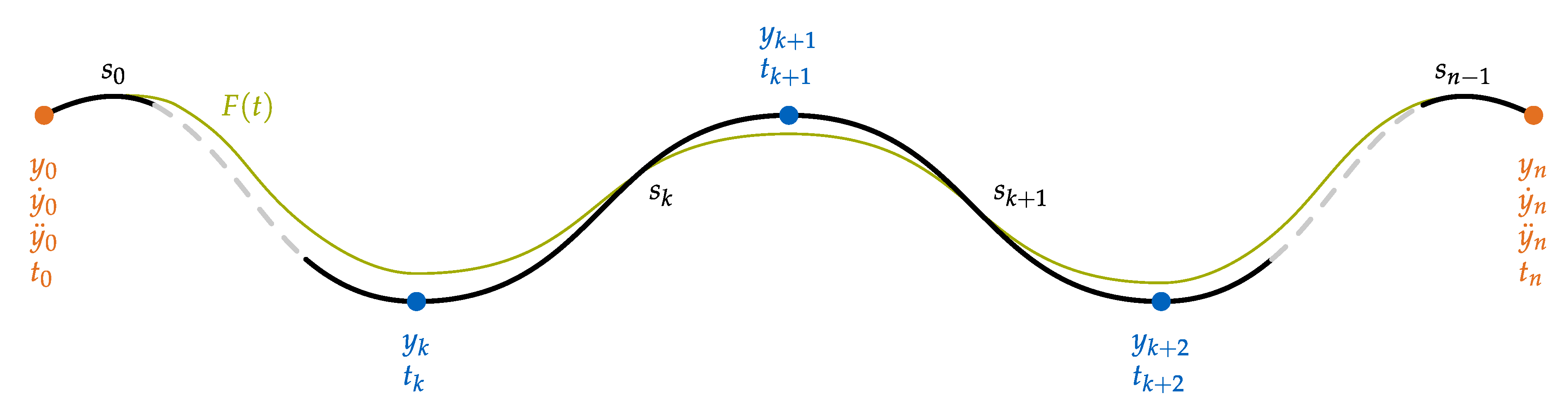
As stated in Section 2.1, we require the approximation to fulfill the underlying ODE at certain collocation sites , see (3), while simultaneously satisfying the boundary conditions as specified in (4). Note that we use the index k instead of i to highlight that our new task consists in collocating the ODE at the interior knots, i.e., rather than the previously investigated interpolation at all knots, i.e., . Furthermore, it should be pointed out that although (3) holds, this does not imply that , , or . In other words, will not coincide with the real solution at the collocation sites . However, it will behave similarly at these spots (meaning that they will satisfy the same Equation (1)), which is illustrated in Figure 4.
As first step, we introduce the auxiliary variables , , and which are defined as
where , , and , , are the corresponding counterparts for the case of cubic and quintic splines, respectively. While represents the (yet unknown) collocation points , contains their corresponding first (and second) time derivatives, which can be seen as “internal” unknowns, as they will be implicitly defined through an embedded spline interpolation. Lastly, depicts the BCs, where we lack and in the case of cubic splines as has been previously explained.
From (17), (30), and (43) we observe that the spline segments are linear with respect to , , and , i.e.,
holds. The gradients are fully defined by the spline partitioning , which is assumed to be known. Thus the construction of the spline is equivalent to the search for a corresponding and . Note that to obtain (44), we used (17) and (30), which in turn were derived from fulfilling the interpolation condition together with enforcing continuity of the second time derivative (cubic spline), or first and second time derivative (quintic spline) at the interior knots. In order to accomplish full and continuity, we further make use of from (19) and (33), which represents continuity of the first time derivative (cubic spline) or third and fourth time derivative (quintic spline), respectively. In particular, we observe from (23), (24), (37), and (38), that is linear with respect to and , thus
holds, where the gradients again depend only on the known partitioning . We further observe that, according to the definitions (21), (35) and (43), we can write the mapping
with being the identity matrix of appropriate size. Since and are constant, by “constant” we mean in this context that an expression does not depend on the yet unknown or , and assumed to be non-singular, it is clear from (45) that not only , but also and thus are linear with respect to and . Hence one can write
Note that and only depend on the known , which allows us to safely differentiate (45) with respect to and to obtain
which we can use to compute the yet unknown gradients in (47). Note that this can be done very efficiently due to the (block-)tridiagonal form of as already discussed in Section 2.3. Since is diagonal, this property also holds for the product . However, for best numerical stability, one should solve for the gradients of first and use the mapping (46) to obtain the gradients of afterwards, which is of negligible cost since , and thus also , is diagonal. The right-hand sides necessary to solve (48) only depend on and are derived in Appendix B. Lastly, we insert from (47) into (44) and obtain
or equivalently
with the known spline gradients
We can obtain the corresponding expressions for the first and second time derivatives by following the exact same scheme. In particular, we get
with
Although computing the spline gradients can be done very efficiently, their mathematical representation is rather lengthy. A formulation of the gradients, which is ready for implementation, is given in Appendix B.
Lastly, we fulfill the dynamics of the ODE by inserting (50) and (52) into (3), which leads to
for and with . This can be formulated as LSE
with
where the k-th row of and corresponds to the collocation site and is given by
Note that we choose a partitioning of the spline such that the collocation sites coincide with the starting (“left”) knot of each segment, i.e., , see Figure 4. This allows us to skip the computation of certain spline gradients. Since the underlying ODE is of order two, only gradients of the last three coefficients, i.e., , , (cubic) or , , (quintic), have to be computed, for details see Appendix B. This simplifies the implementation and improves the overall performance. Solving (56) for represents the key operation (i.e., bottleneck for large n) of the proposed collocation method, since is in general dense while all other operations are either simple explicit expressions or linear systems in (block-)tridiagonal form, which can be solved efficiently. This justifies our strategy to minimize the count of collocation points (and thus the dimension of ) and instead force high order continuity.
2.8. Satisfying First Order Boundary Conditions for Cubic Splines
The presented method for cubic spline collocation respects , , , and as BCs. However, our task was to fulfill all BCs given in (4), which seems at first to be only possible with quintic spline collocation. Also satisfying the first-order BCs, i.e., and , can be achieved with moderate effort. For that purpose we insert two auxiliary knots, the so-called virtual control points and , which give us the necessary degrees of freedom to introduce additional constraints. The term “virtual” highlights that these points are not used as collocation sites. Both, and , have to lie within the specified start- and endtime and must not coincide with the collocation sites. This way the spline remains properly partitioned. For simplicity, we place the virtual control points at the centers of the (originally) first and last segments, i.e.,
Obviously, inserting two knots leads to a different segmentation of the spline, i.e., ; however, the boundaries and collocation sites remain unchanged. If we adapt the indexing such that and , all findings derived so far are also valid for this case. The only difference is that we do not force to fulfill the underlying ODE at and anymore. Instead, we satisfy the BCs and by replacing the first and last row of and with
In this way the resulting cubic spline fulfills all BCs given in (4), satisfies the underlying ODE at the specified collocation sites, and is continuous at the interior spline knots (which include and ).
2.9. Algorithm for Cubic/Quintic Spline Collocation
We summarize our findings in Algorithm 2. Note that, for the case of cubic splines, the modification necessary to satisfy first-order BCs is already integrated.
| Algorithm 2: Cubic/Quintic Spline Collocation. |
 |
3. Results
3.1. Implementation
Algorithm 2 delivers a detailed description of the proposed collocation method which can be used as a reference during implementation. However, we also provide a fully documented C++ implementation through our free and open-source library BROCCOLI [34] (see Supplementary Materials). For best usability, the library is designed to be header-only and uses the (also header-only) cross-platform linear algebra system EIGEN [35] as sole dependency. Although BROCCOLI also has other dependencies, only EIGEN is required for the functionality discussed in this paper. Aside from basic matrix and vector operations, we use EIGEN to solve dense linear systems of equations such as in (56), but also and in (40) and (41). In particular, we use a Householder rank-revealing QR decomposition with column-pivoting, see ColPivHouseholderQR in EIGEN, since it provides the best trade-off between speed, accuracy, and robustness for our use case. Note that for large scale systems solving turns out to be the bottleneck, cf. Figure 11. Thus, in this case one might choose a parallel solver for (56) instead, for example PartialPivLU in EIGEN with OPENMP enabled. In addition to the variants CubicSplineCollocator and QuinticSplineCollocator for spline collocation, see ode module of BROCCOLI, cubic and quintic spline interpolation, see curve module of BROCCOLI, as specified in Algorithm 1, is also implemented. An overview over the structure of the source code related to our collocation method is given in Appendix C. Lastly, unit tests, similar to the evaluation presented in the following, are shipped with BROCCOLI. These can be used as example applications.
3.2. Test System
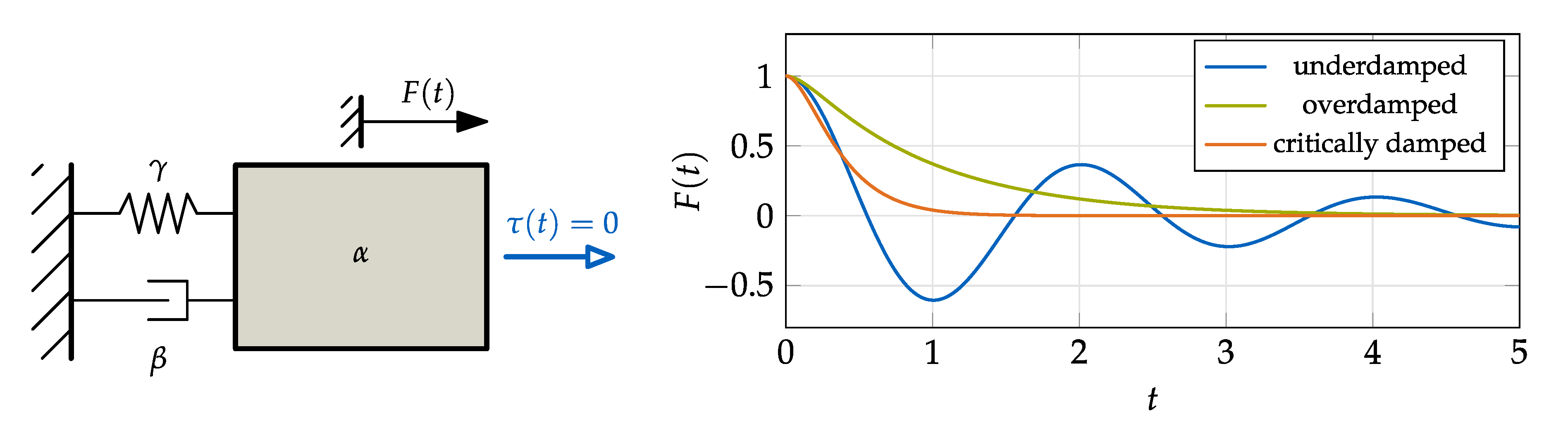
In order to evaluate the proposed method and its variants, a simple mass-spring-damper system is considered, see Figure 5 (left). For the sake of simplicity, we do not consider external excitation, i.e., . The corresponding ODE (1) describing the system dynamics simplifies to
where , , and are constants representing the mass and (linear) damping/stiffness coefficients of the system, respectively.
Using textbook mathematics, we can find the analytical solution given by
where we used the initial conditions and , and the abbreviations
The characteristic shape of each branch of (63) is visualized in Figure 5 (right) for the parametrization , , in the underdamped case, , , in the overdamped case, and , , in the critically damped case. For the rest of this paper we will adhere to this parametrization. Moreover, we assume the initial conditions to be given with , . Note that by choosing we obtain asymptotically stable behavior. As we never constrained the underlying ODE to be stable, our algorithm can also be used to approximate instable systems. Since tests with showed results comparable to the underdamped case (with ), we omit an explicit discussion of this case for brevity. Lastly, we point out that although (62) describes a very simple system, we also successfully applied the proposed algorithm to the much more complex walking-pattern generation system of our humanoid robot LOLA, cf. [13]. However, the properties and characteristics of the proposed method can be better investigated and explained by means of a less complex test system.
3.3. Convergence for Consistent and Inconsistent Boundary Conditions
As already mentioned, we focus on over-determined BVPs. Thus, we consider two cases for evaluating our algorithm. For the first analysis, we use the initial conditions , and correspondingly , see (62), together with the analytical solution given in (63) to compute the BCs , , and at . In this way, the BCs are guaranteed to be consistent because they belong to the same analytic solution . In the second case, we keep the initial BCs unchanged, but force for which deviates from the previous solution , , and , especially in the underdamped case, as can be clearly seen in Figure 5 right. Thus, the second analysis handles inconsistent BCs.
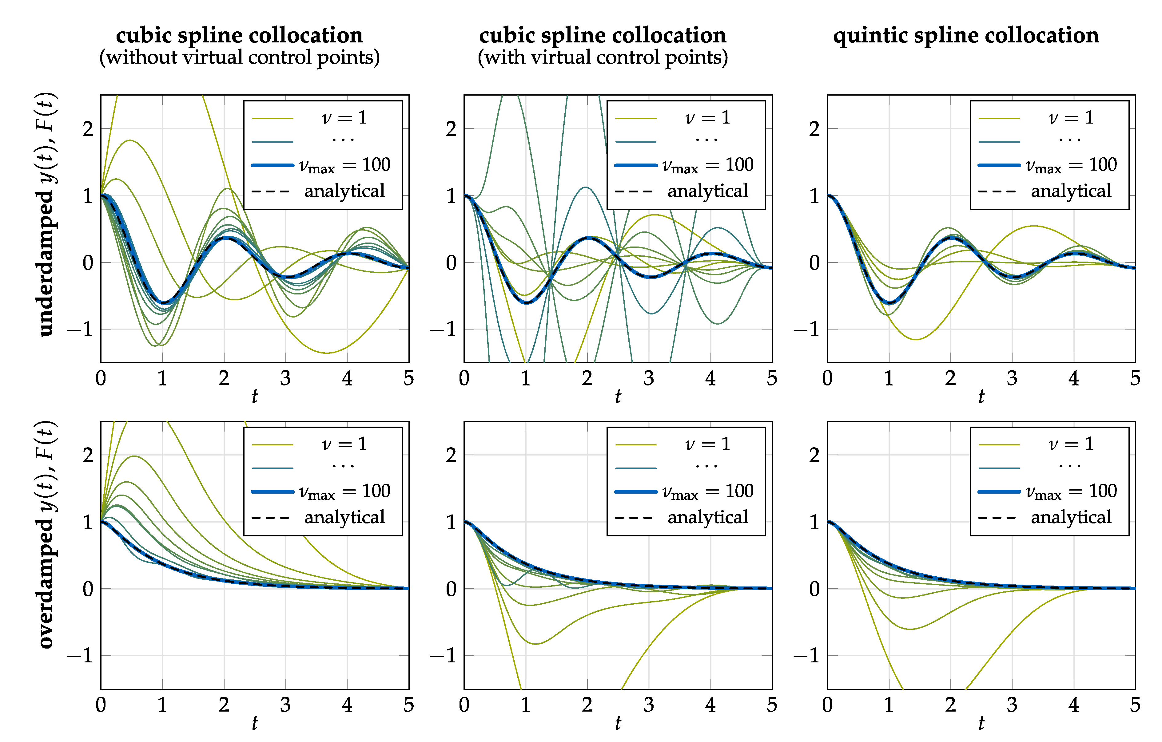
In the following, we only focus on the underdamped and overdamped case, since the critically damped case can be seen as a special form of these with . By evaluating both cases, we aim at covering oscillating and non-oscillating dynamics. Moreover, we run tests for different counts of collocation sites , where we use a uniform segmentation of the spline, i.e., . For cubic and quintic spline collocation without virtual control points holds. In contrast, holds for cubic spline collocation with virtual control points. Note that an inhomogeneous partitioning is evaluated per default in the unit tests provided with BROCCOLI. The approximation of the BVP by spline collocation with consistent BCs and is depicted in Figure 6. Note that for cubic spline collocation without virtual control points, the BCs and are violated (see Section 2.7).
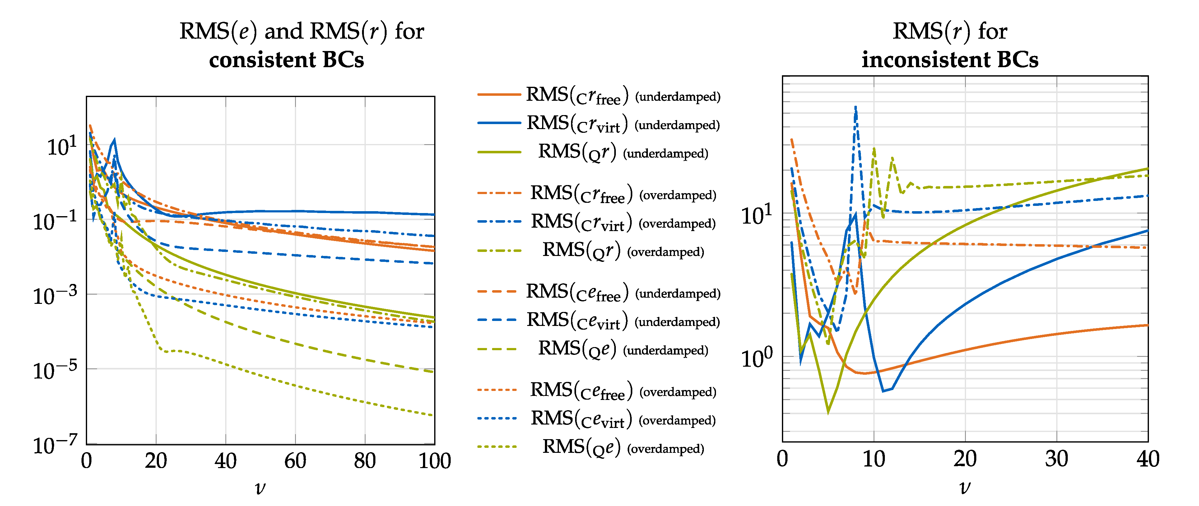
For the case of consistent BCs, we observe that the approximation indeed converges for increasing to the analytical solution . From a qualitative point of view, the convergence order using a quintic spline (Figure 6 right column) is clearly higher than the corresponding cubic counterparts (Figure 6 left and center column). In order to compare convergence using a quantitative measure, we use the root mean square (RMS) of the approximation error and of the residual , defined as
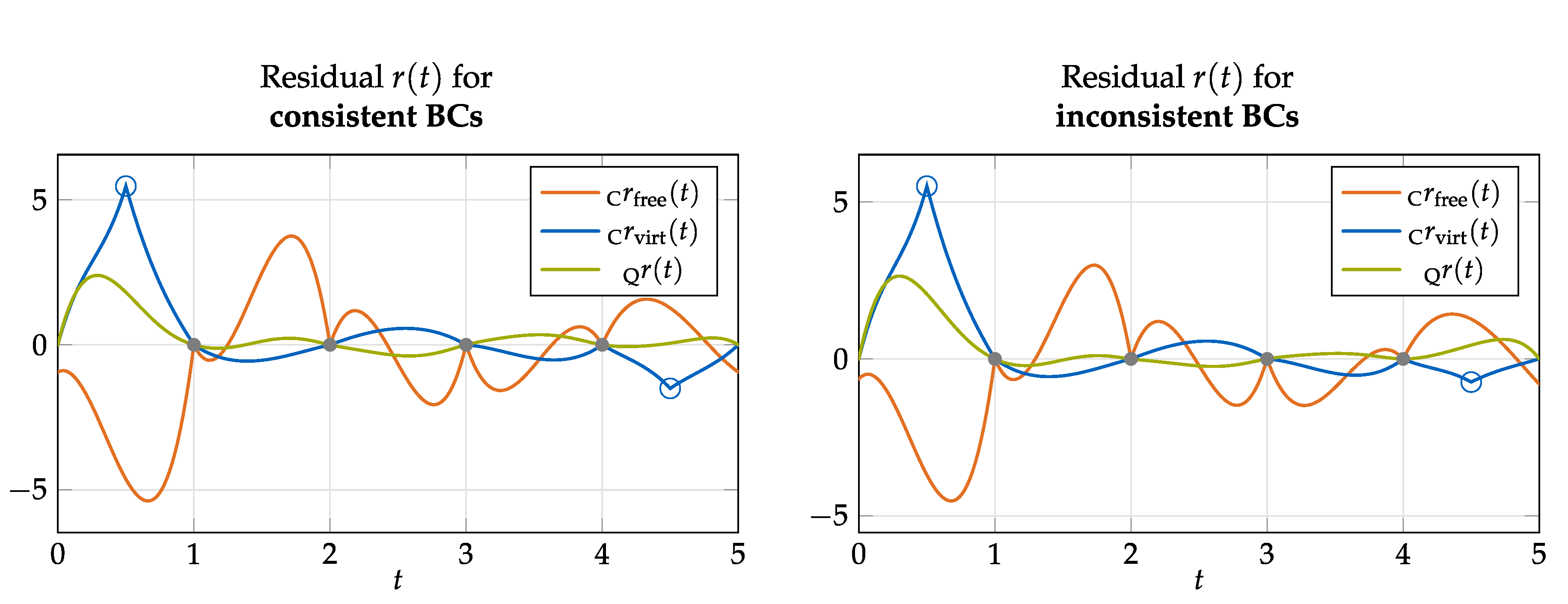
For numerical evaluation of (65) and (66), we discretize the embedded integral using a time step size of for which we obtain the results presented in Figure 7 left. Since we stop the test series at , we find the optimum for all variants to be at . However, due to convergence, we expect the theoretical optimum to be at . We observe that also from an quantitative point of view, quintic spline collocation clearly outperforms the cubic variants for the same . Furthermore, forcing first-order BCs through virtual control points of the cubic spline seems to have a negative influence, especially for increasing . The influence of virtual control points on the residual is visualized in Figure 8 where peaks in occur at these spots. Note that without virtual control points, the first-order boundary conditions at and are missed. Thus, in contrast to the collocation sites, the residual does not drop to zero at the boundaries. By comparing the left and right plot of Figure 8, we observe that behaves similarly for consistent and inconsistent BCs.
For consistent BCs, we can state that, at least for the investigated test system, the proposed algorithm leads to an approximation which converges to the real solution where the “speed” of convergence depends on the chosen variant of 2. For inconsistent BCs, however, our analysis draws a different picture: while we can find an optimal count of collocation sites for each variant and test case, the approximation diverges for , see Figure 7 right and Figure 9. Note that this was expected since we are attempting to find an approximation of a solution which does not actually exist. For small , we still find a “reasonable” where the spline is still able to smooth out the wrong BCs. However, as we refine the segmentation of the spline, it gets harder to compensate the error, which in turn leads to undesired oscillations of . Note that although we call this behavior divergence, our collocation algorithm still satisfies all constraints that we defined: using a given partitioning, it fulfills the BCs and satisfies the underlying ODE at the given collocation sites. Thus, the divergence is not a fault of the proposed algorithm, but rather is due to the non-existence of the solution . Moreover, the sensitivity to undesired oscillations depends heavily on the underlying BVP: for our target application of real-time motion planning, we did not observe any oscillations up to . The critical value for is expected to be even higher. However, we could not determine it due to memory limitations of our test system.
In order to avoid undesired oscillations, an optimal has to be chosen, which seems to be difficult at the first sight, since in practice we do not know the analytical solution, and thus cannot evaluate . However, one can use the residual as measure for the approximation error and use this to formulate a governing optimization for finding . Moreover, one can also use a non-uniform segmentation to give specific sections more weight. Such adaptive techniques for automatic mesh refinement have also been developed for other collocation methods, see, for example, [36]. However, for our application it is sufficient to choose once (fixed), thus we withhold this idea for future investigations.
3.4. Runtime Analysis
In the following, we present measurements, which have been made by using the implementation given in BROCCOLI with the version primo (v1.0.0 - commit 89280c69). We used an AMD Ryzen 7 1700X 8x (16x) @3.40GHz with 32GB DDR4 RAM @2133MHz as hardware backend and Ubuntu 18.04.2 LTS 64bit (Linux kernel 4.15.0-51) together with Clang (version 6.0.0-1) on optimization level 3 as software basis. Although our algorithm is sequential, we run different test cases on four physical cores of the CPU in parallel. For all tests simultaneous multi-threading (SMT) was disabled in the BIOS. For runtime evaluation, we take 1000 samples for every code section in Algorithm 2 and choose the minimum execution time as reference to minimize the risk of wrong measurements due to high system load and context switching effects.
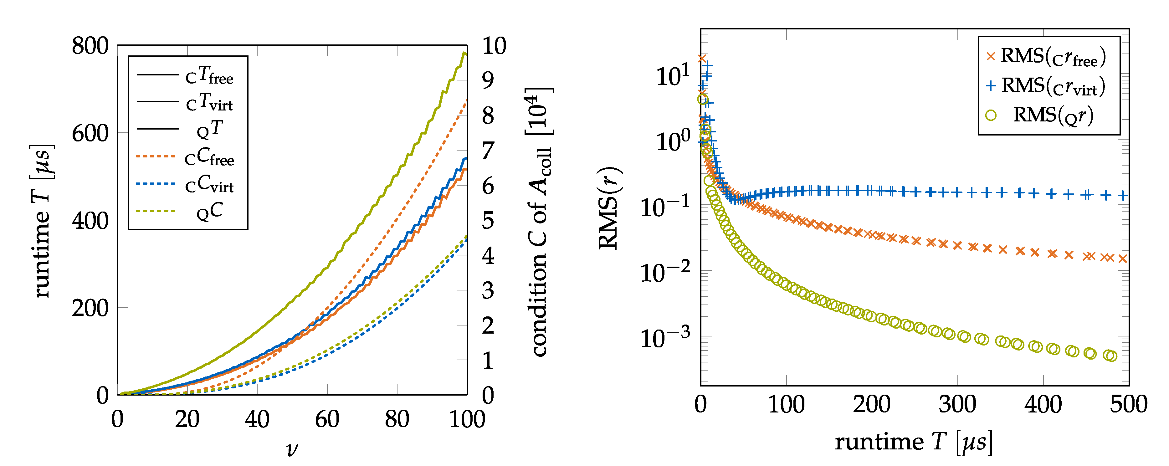
In Figure 10 (left), we present runtime measurements for all three variants of our algorithm. We restrict our analysis to the case of an underdamped parametrization and consistent BCs since we expect comparable results for the other test cases. Since our algorithm has a deterministic runtime which only depends on the chosen variant (cubic/quintic, with/without virtual control points) and , there is no reason why it should be faster or slower with another parametrization. We observe that quintic spline collocation is more expensive than the cubic counterparts for the same , which complies with theory since the (block-)tridiagonal system for quintic splines is twice the size of the tridiagonal system for cubic splines. However, for increasing , the gap becomes smaller since solving the collocation equations, where is of the same dimension for cubic and quintic splines, becomes the bottleneck, see Figure 11. Note that there is only a small difference in runtime between cubic spline collocation with and without virtual control points. This also complies with theory, since the only difference is two additional spline knots, which increases the dimension of by two. Lastly, the small ripples in Figure 10 (left) are due to vectorization and SIMD optimizations handled by EIGEN and the compiler, which give slightly better performance if the dimension of arrays in memory are a multiple of two.
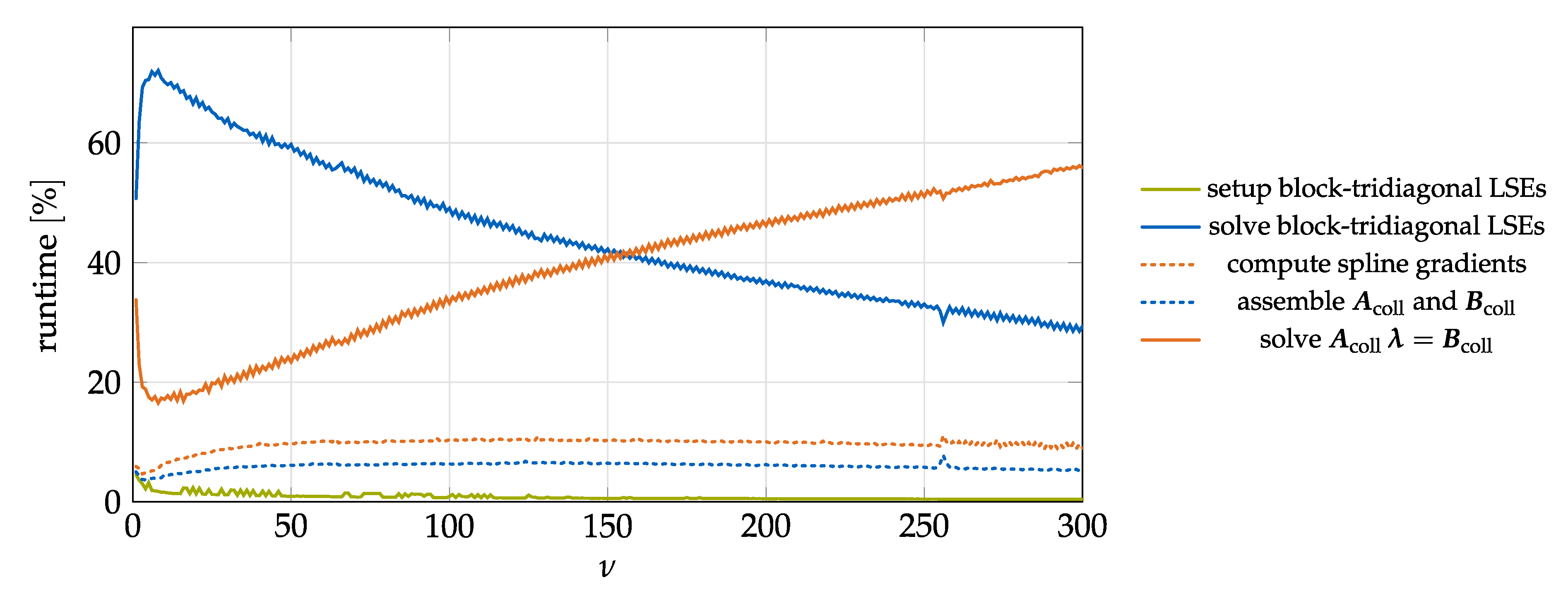
Comparing runtimes for the same might not be a meaningful basis for choosing a method. Instead, one is typically interested in getting the best approximation in the shortest time. For this purpose, the RMS of the residual is plotted over runtime in Figure 10 (right). As can be seen, quintic spline collocation significantly outperforms both other variants. Moreover, bad convergence of cubic spline collocation with virtual control points is also visible in this comparison. In addition to measuring total runtime, we also performed a detailed analysis on the relative cost of each code section of Algorithm 2 during quintic spline collocation. Figure 11 demonstrates that in the vicinity of , evaluating the block-tridiagonal systems to enforce BCs and continuity, and solving for actual collocation share approximately the same portion of total runtime. With increasing , solving for becomes more relevant since the corresponding system is dense while the block-tridiagonal LSE can be solved efficiently using the recursive scheme discussed in Section 2.3.
Lastly, we want to point out that the condition of gets worse for increasing count of collocation sites , see Figure 10 left. Thus, there might be an upper limit of for the proposed algorithm.
4. Discussion
As shown in the previous section, the presented algorithm performs well if the BCs are consistent and fully known. Even in the case of inconsistent BCs, we still obtain a reasonable approximation as long as we carefully pick the collocation sites. However, if we exceed the optimum, undesired oscillations may occur, which is an indicator for putting too much emphasis on satisfying the underlying ODE while simultaneously trying to compensate the “broken” BCs. In order to automatically determine an optimal partitioning of the spline, a higher level optimization may be applied, which will be the focus of further investigations.
Obviously, if the investigated BVP is well-posed, i.e., if it is not over-determined, other techniques should be preferred over our approach. However, for applications where the enforcement of certain BCs is more important than approximating the underlying dynamics, the proposed method seems to be a valid approach. Moreover, we want to emphasize that no variable recursion or iteration is involved. This makes execution time predictable, which is especially relevant for real-time applications such as in our use case.
Comparing different variants of our algorithm showed that collocation using a quintic spline is in general superior to using the somewhat simpler cubic splines. Note that although its derivation is more involved, the final implementation is of approximately the same complexity, since virtual control points have to be introduced in the cubic case. At this point, we also want to emphasize that, based on the results of our study, we do not recommend to use cubic spline collocation with virtual control points. Although the full set of BCs is satisfied, the additional knots seem to significantly downgrade convergence. However, other choices of and may lead to different results.
Within this contribution, we only considered second-order BVPs. An extension to ODEs of higher order seems to be straightforward, since only the collocation equations, see (58) and (59) have to be extended by the corresponding gradients while the overall dimension of and stays the same. Moreover, our approach may be applied to nonlinear systems as well, by using the common approach of linearization and embedding the scheme into a Newton iteration.
Lastly, we want to highlight that our focus lies on runtime efficiency. However, for embedded systems especially, memory consumption may also be a limiting factor. Although we expect our algorithm to have similar requirements when compared to other techniques, we have not looked into this issue so far.
Supplementary Materials
An archived version of the free and open-source C++ header-only library BROCCOLI in the version primo (v1.0.0) which includes the proposed algorithm is available online at https://www.mdpi.com/2218-6581/9/2/48/s1. For the most recent version of BROCCOLI visit https://gitlab.lrz.de/AM/broccoli.
Author Contributions
Conceptualization, P.S.; Data curation, P.S.; Formal analysis, P.S.; Funding acquisition, D.J.R.; Investigation, P.S.; Methodology, P.S.; Project administration, D.J.R.; Resources, P.S.; Software, P.S.; Supervision, D.J.R.; Validation, P.S.; Visualization, P.S.; Writing—original draft, P.S.; Writing—review & editing, P.S. and D.J.R. All authors have read and agreed to the published version of the manuscript.
Funding
This work was supported by the German Research Foundation (DFG), project number 407378162. Moreover, this work was supported by the DFG and the Technical University of Munich (TUM) in the framework of the Open Access Publishing Program.
Acknowledgments
We would like to express special thanks to Nora-Sophie Staufenberg and Felix Sygulla for the constructive discussions during development, implementation and analysis of the presented method.
Conflicts of Interest
The authors declare no conflict of interest. The funders had no role in the design of the study; in the collection, analyses, or interpretation of data; in the writing of the manuscript, or in the decision to publish the results.
Abbreviations
The following abbreviations are used in this manuscript:
| BVP | Boundary Value Problem |
| IVP | Initial Value Problem |
| PDE | Partial Differential Equation |
| ODE | Ordinary Differential Equation |
| DAE | Differential Algebraic Equation |
| BC | Boundary Condition |
| CoM | Center of Mass |
| ABD | Almost Block Diagonal |
| LSE | Linear System of Equations |
| PP | Piecewise Polynomial |
| RMS | Root Mean Square |
| SMT | Simultaneous Multi-Threading |
| DFG | German Research Foundation (Deutsche Forschungsgemeinschaft) |
| TUM | Technical University of Munich |
Appendix A. Considerations on Numerical Stability
Appendix A.1. Cubic Spline Interpolation
The Thomas algorithm is guaranteed to be numerically stable if is diagonally dominant, i.e., if
holds [30], whereas for and we use and , respectively. As is easily verified with (A1), this holds true for any choice of and (i.e., for distinct and ascending interpolation sites), thus the presented method is always stable.
Appendix A.2. Quintic Spline Interpolation
The presented scheme for solving block-tridiagonal systems is a special form of block-Gaussian elimination without pivoting and is guaranteed to be numerically stable if is block-diagonally dominant, i.e., if
holds for an arbitrary matrix norm [37]. Note that for and we set and , respectively. In order to verify (A2) for , , and as specified in (35) and (36), we assume a constant ratio to obtain
and further
which shows that does not depend on for a constant ratio . It can be easily verified through numerical evaluation of (A4) that a homogeneous partitioning of the spline, i.e., , results in the lowest value for . Using the spectral matrix norm and the special choice of given in (39) leads to
Unfortunately, condition (A2) is violated, even for the ideal case of a homogeneously partitioned spline. However, (A2) represents a sufficient but not necessary condition for numerical stability, thus we can still use as a measure for the pivotal growth [37] which should be minimized. In doing so, we can conclude that for best numerical stability one should use a “reasonable” ratio which is close to 1.
Note that the special choice of in (39) has been suggested in [18] to minimize and thus optimize numerical stability. This intention becomes clear when observing that
where denotes the maximum eigenvalue of a given matrix. Since both and , increase with growing , the optimum (39) is chosen. This finding can be easily verified through numerical investigation. Note that numerical stability only depends on , thus one could also choose the negative form .
Appendix B. Spline Gradients
In the following, explicit expressions for the spline gradients used in (51), (53), and (54) are given. Note that the gradients differ depending on the type of the underlying spline (cubic/quintic).
Appendix B.1. Cubic Spline Gradients
Moreover, by using the indices , , and to specify the elements of
we obtain
which can easily be derived from (17) and the definition of , , and . Note that for the computation of
can be skipped entirely since up to the second time derivative of the gradients of these terms are multiplied with zero and have no effect anyway. In order to solve (48), we have to further compute the corresponding right-hand sides which are given by
for , where we used (23), (24), and the definition of and .
Appendix B.2. Quintic Spline Gradients
Moreover, by using the indices , , and to specify the elements of
we obtain
which can easily be derived from (30) and the definition of , , and . Note that for the computation of
can be skipped entirely since up to the second time derivative of the gradients of these terms are multiplied with zero and have no effect anyway. In order to solve (48), we further have to compute the corresponding right-hand sides, which are given by
for , where we used (37), (38), and the definition of and .
Appendix C. Software Design in BROCCOLI
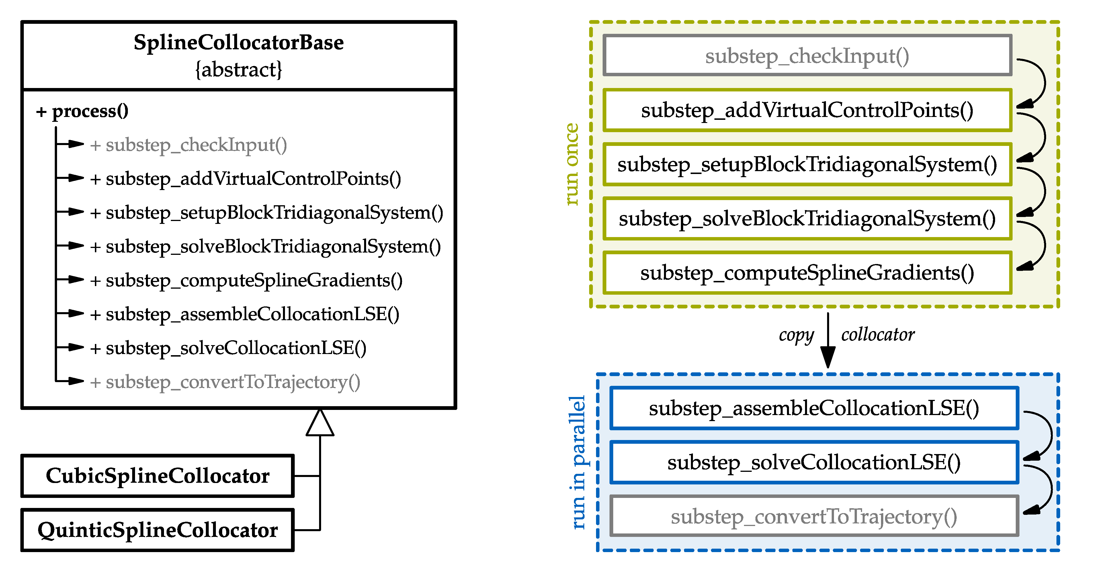
The basic structure of the source code related to the classes CubicSplineCollocator and QuinticSplineCollocator is illustrated in Figure A1 (left). Both classes are derived from the abstract base class SplineCollocatorBase, which declares the interface for data in-/output and the main processing operators. In order to trigger Algorithm 2 for a given input dataset, a simple call of process() is sufficient. For a more fine-grained control, process() is split up into publicly available subroutines (names starting with “substep_”). Note that providing public access to the subroutines not only allows detailed runtime measurements by the user, but also enables an efficient parallel solution for decoupled, multi-dimensional BVPs, see Figure A1 right. For this, we exploit that large parts of Algorithm 2 only depend on the spline segmentation, i.e., the collocation sites, (green box). In contrast, the remaining subroutines require explicit information about the investigated BVP (blue box). If all dimensions of the BVP, e.g., the x- and y-component of LOLA’s CoM motion, share the same spline segmentation, subroutines covered by the green box in Figure A1 have to be called only once. Subsequently, the used instance of CubicSplineCollocator or QuinticSplineCollocator (holding intermediate results) is copied such that the remaining subroutines, covered by the blue box in Figure A1, can be run in parallel. Note that this includes solving (substep_solveCollocationLSE()), which is the bottleneck for large-scale systems. We plan to use this feature in our target application to efficiently generate the CoM motion of LOLA (the x- and y-component represent a decoupled, two-dimensional BVP).
Figure A1.
Design of the classes CubicSplineCollocator and QuinticSplineCollocator in BROCCOLI. Left: class inheritance and segmentation of process() into subroutines. Right: proposed strategy for efficient parallelization in the case of a decoupled, multi-dimensional BVP. Note that the first and last subroutine (grayed out) are optional and perform a validity check of the given input parameters and convert the final result into a corresponding broccoli::curve::Trajectory data structure for convenient evaluation of the generated polynomial spline, respectively.

References
- Lee, J.F.; Lee, R.; Cangellaris, A. Time-Domain Finite-Element Methods. IEEE Trans. Antennas Propag. 1997, 45, 430–442. [Google Scholar]
- Ahlberg, J.H.; Nilson, E.N.; Walsh, J.L. The Theory of Splines and Their Applications; Mathematics in Science and Engineering; Academic Press: New York, NY, USA, 1967. [Google Scholar]
- De Boor, C.; Swartz, B. Collocation at Gaussian Points. SIAM J. Numer. Anal. 1973, 10, 582–606. [Google Scholar] [CrossRef]
- Ahlberg, J.; Ito, T. A Collocation Method for Two-Point Boundary Value Problems. Math. Comput. 1975, 29, 761–776. [Google Scholar] [CrossRef]
- Christara, C.C.; Ng, K.S. Optimal Quadratic and Cubic Spline Collocation on Nonuniform Partitions. Computing 2005, 76, 227–257. [Google Scholar] [CrossRef]
- Bialecki, B.; Fairweather, G. Orthogonal spline collocation methods for partial differential equations. J. Comput. Appl. Math. 2001, 128, 55–82. [Google Scholar] [CrossRef] [Green Version]
- Houstis, E.N.; Christara, C.C.; Rice, J.R. Quadratic-Spline Collocation Methods for Two-Point Boundary Value Problems. Int. J. Numer. Methods Eng. 1988, 26, 935–952. [Google Scholar] [CrossRef] [Green Version]
- Irodotou-Ellina, M.; Houstis, E.N. An O(h6) Quintic Spline Collocation Method for Fourth Order Two-Point Boundary Value Problems. BIT Numer. Math. 1988, 28, 288–301. [Google Scholar] [CrossRef]
- Ascher, U. Solving Boundary-Value Problems with a Spline-Collocation Code. J. Comput. Phys. 1980, 34, 401–413. [Google Scholar] [CrossRef]
- Zhang, H.; Han, X.; Yang, X. Quintic B-spline collocation method for fourth order partial integro-differential equations with a weakly singular kernel. Appl. Math. Comput. 2013, 219, 6565–6575. [Google Scholar] [CrossRef]
- Akram, G.; Tariq, H. Quintic spline collocation method for fractional boundary value problems. J. Assoc. Arab Univ. Basic Appl. Sci. 2017, 23, 57–65. [Google Scholar] [CrossRef] [Green Version]
- Ascher, U.; Spiteri, R. Collocation Software for Boundary Value Differential-Algebraic Equations. SIAM J. Sci. Comput. 1995, 15. [Google Scholar] [CrossRef]
- Seiwald, P.; Sygulla, F.; Staufenberg, N.S.; Rixen, D. Quintic Spline Collocation for Real-Time Biped Walking-Pattern Generation with variable Torso Height. In Proceedings of the IEEE-RAS 19th International Conference on Humanoid Robots (Humanoids), Toronto, ON, Canada, 15–17 October 2019; pp. 56–63. [Google Scholar]
- Seiwald, P. Video: Smooth Real-Time Walking-Pattern Generation for Humanoid Robot LOLA. Available online: https://youtu.be/piQm_oTYXIc (accessed on 22 June 2020).
- Wright, S.J. Stable Parallel Algorithms for Two-Point Boundary Value Problems. SIAM J. Sci. Statistical Comput. 1992, 13, 742–764. [Google Scholar] [CrossRef]
- Magoulés, F.; Roux, F.X.; Houzeaux, G. Parallel Scientific Computing; Wiley & Sons: New York, NY, USA, 2015. [Google Scholar]
- Usmani, R.A. Smooth spline approximations for the solution of a boundary value problem with engineering applications. J. Comput. Appl. Math. 1980, 6, 93–98. [Google Scholar] [CrossRef] [Green Version]
- Mund, E.H.; Hallet, P.; Hennart, J.P. An algorithm for the interpolation of functions using quintic splines. J. Comput. Appl. Math. 1975, 1, 279–288. [Google Scholar] [CrossRef] [Green Version]
- Buschmann, T.; Lohmeier, S.; Bachmayer, M.; Ulbrich, H.; Pfeiffer, F. A Collocation Method for Real-Time Walking Pattern Generation. In Proceedings of the IEEE-RAS 7th International Conference on Humanoid Robots, Pittsburgh, PA, USA, 29 November–1 December 2007; pp. 1–6. [Google Scholar]
- Ascher, U.; Pruess, S.; Russell, R.D. On Spline Basis Selection for Solving Differential Equations. SIAM J. Numer. Anal. 1983, 20, 121–142. [Google Scholar] [CrossRef]
- De Boor, C. A Practical Guide to Splines; Springer: New York, NY, USA, 2001; ISBN 978-0387953663. [Google Scholar]
- De Boor, C.; Weiss, R. SOLVEBLOK: A Package for Solving Almost Block Diagonal Linear Systems. ACM Trans. Math. Software 1980, 6, 80–87. [Google Scholar] [CrossRef]
- Majaess, F.; Keast, P.; Fairweather, G. The Packages for solving almost block diagonal linear systems arising in spline collocation at Gaussian points with monomial basis functions. In Scientific Software Systems; Springer: Dordt, The Netherlands, 1988; pp. 47–58. [Google Scholar]
- De Boor, C. On calculating with B-splines. J. Approximation Theor. 1972, 6, 50–62. [Google Scholar] [CrossRef] [Green Version]
- Böhm, W. Efficient Evaluation of Splines. Computing 1984, 33, 171–177. [Google Scholar] [CrossRef]
- Lee, E.T.Y. A Simplified B-Spline Computation Routine. Computing 1982, 29, 365–371. [Google Scholar] [CrossRef]
- Lee, E.T.Y. Comments on Some B-Spline Algorithms. Computing 1986, 36, 229–238. [Google Scholar] [CrossRef]
- Horner, W.G.; Gilbert, D. A New Method of Solving Numerical Equations of All Orders, by Continuous Approximation; Philosophical Transactions of the Royal Society of London: London, UK, 1819; pp. 308–335. [Google Scholar]
- Higham, N.J. Accuracy and Stability of Numerical Algorithms, 2nd ed.; Society for Industrial and Applied Mathematics: Philadelphia, PA, USA, 2002. [Google Scholar]
- Quarteroni, A.; Sacco, R.; Saler, F. Numerical Mathematics, 2nd ed.; Springer: Berlin, Germany, 2007. [Google Scholar]
- Isaacson, E.; Keller, H.B. Analysis of Numerical Methods; Dover Publications, Inc.: New York, NY, USA, 1966. [Google Scholar]
- Meurant, G. A Review on the Inverse of Symmetric Tridiagonal and Block Tridiagonal Matrices. SIAM J. Matrix Anal. Appl. 1992, 13, 707–728. [Google Scholar] [CrossRef] [Green Version]
- Buschmann, T. Simulation and Control of Biped Walking Robots. Ph.D. Thesis, Technical University of Munich, Munich, Germany, November 2010. Available online: https://mediatum.ub.tum.de/997204 (accessed on 22 June 2020).
- Seiwald, P.; Sygulla, F. Broccoli: Beautiful Robot C++ Code Library. Available online: https://gitlab.lrz.de/AM/broccoli (accessed on 22 June 2020).
- Guennebaud, G.; Jacob, B. Eigen. Available online: http://eigen.tuxfamily.org (accessed on 22 June 2020).
- Christara, C.C.; Ng, K.S. Adaptive Techniques for Spline Collocation. Computing 2006, 76, 259–277. [Google Scholar] [CrossRef]
- Varah, J.M. On the Solution of Block-Tridiagonal Systems Arising from Certain Finite-Difference Equations. Math. Comput. 1972, 26, 859–868. [Google Scholar] [CrossRef]
Figure 1.
Humanoid robot LOLA developed at the Lehrstuhl für Angewandte Mechanik, Technical University of Munich (TUM). The proposed algorithm is used within the walking pattern generation framework of LOLA, see [13] for details. The robot is tall and weights about 60 . Left: photo and kinematic configuration of the system with 24 actuated degrees of freedom. Right: simplified model of multi-body dynamics with torso mass , foot mass and torso mass moment of inertia which (together with the ground reaction forces/torques) contribute to the ordinary differential equation (ODE) describing the center of mass (CoM) dynamics (blue).

Figure 2.
Visual interpretation of the over-determined boundary value problem (BVP): the start and end pose (left/right) represent the boundary conditions, while the intermediate motion (transparent) tries to approximate the inherent system dynamics of the simplified model.
Figure 2.
Visual interpretation of the over-determined boundary value problem (BVP): the start and end pose (left/right) represent the boundary conditions, while the intermediate motion (transparent) tries to approximate the inherent system dynamics of the simplified model.

Figure 3.
Segmentation and parametrization of the investigated spline . The spline consists of n interconnected segments, which share the interior knots with their neighbors. Each segment is described through the local interpolation parameter (blue).
Figure 3.
Segmentation and parametrization of the investigated spline . The spline consists of n interconnected segments, which share the interior knots with their neighbors. Each segment is described through the local interpolation parameter (blue).

Figure 4.
The computed spline (black) approximating the real solution (green). The approximation satisfies the underlying ODE at the specified collocation sites (blue), and fulfills the boundary conditions (BC) at and (orange), but do not necessarily coincide at the collocation points.
Figure 4.
The computed spline (black) approximating the real solution (green). The approximation satisfies the underlying ODE at the specified collocation sites (blue), and fulfills the boundary conditions (BC) at and (orange), but do not necessarily coincide at the collocation points.

Figure 5.
Left: mass-spring-damper system used for validation. Right: analytical solution for the underdamped case (, , ), the overdamped case (, , ) and the critically damped case (, , ). The solution is plotted for the initial conditions , .
Figure 5.
Left: mass-spring-damper system used for validation. Right: analytical solution for the underdamped case (, , ), the overdamped case (, , ) and the critically damped case (, , ). The solution is plotted for the initial conditions , .

Figure 6.
Consistent BCs: convergence of the approximation (blue and green) towards the analytic solution (black, dashed) for . The top row belongs to the underdamped case while the bottom row represents the overdamped case. From left to right: approximation with cubic spline without virtual control points (left), cubic spline with virtual control points (center) and quintic spline (right). The corresponding best approximation is drawn in bold blue.

Figure 7.
Root mean square (RMS) of error and residual as defined in (65) and (66). The left subscript differs between cubic C and quintic Q spline collocation. Moreover, for cubic spline collocation, we identify the variants without virtual control points (i.e., free first-order boundaries , ) and with virtual control points by the right subscript and , respectively. The left plot belongs to the case of consistent BCs while the right one was obtained using inconsistent BCs. Note that for inconsistent BCs an analytic solution does not exist, thus the error is not defined and we consider only the residual .

Figure 8.
Residual as defined in (66) for consistent (left) and inconsistent (right) BCs in the underdamped case. For best presentation, the count of collocation sites is chosen as such that the collocation sites (dots) are given by . For cubic spline collocation, the left subscript C and for the quintic counterpart Q is used. Moreover, the right subscripts and are used to differentiate between the variants without and with virtual control points, respectively. The virtual control points are highlighted with circles.

Figure 9.
Inconsistent BCs: approximation (blue, green, and orange) and reference system (black, dashed) for . The top row belongs to the underdamped case while the bottom row represents the overdamped case. From left to right: approximation with cubic spline (no virtual control points, left), cubic spline (with virtual control points, center) and quintic spline (right). The corresponding best approximation is drawn in bold blue. Diverging approximations for are colored orange.

Figure 10.
Left: (minimum) runtime T and condition C of for running 2 over count of collocation sites . Right: root mean square (RMS) of residual as defined in (66) over (minimum) runtime T. The left subscript C and Q belong to the cubic or quintic spline version of the algorithm, respectively. Moreover, the right subscript indicates if cubic spline collocation was performed without () or with () virtual control points. All measurements were performed using the underdamped parametrization and consistent BCs.

Figure 11.
Runtime (percentile) of relevant steps of 2 relative to total runtime for quintic spline collocation. Code sections with negligible execution time are not plotted and also not accounted for total runtime. The measurements were obtained by using an extended time horizon and the parametrization , , (underdamped) to allow a better representation of high counts of collocation sites of up to .

© 2020 by the authors. Licensee MDPI, Basel, Switzerland. This article is an open access article distributed under the terms and conditions of the Creative Commons Attribution (CC BY) license (http://creativecommons.org/licenses/by/4.0/).
Share and Cite
MDPI and ACS Style
Seiwald, P.; Rixen, D.J. Fast Approximation of Over-Determined Second-Order Linear Boundary Value Problems by Cubic and Quintic Spline Collocation. Robotics 2020, 9, 48. https://doi.org/10.3390/robotics9020048
AMA Style
Seiwald P, Rixen DJ. Fast Approximation of Over-Determined Second-Order Linear Boundary Value Problems by Cubic and Quintic Spline Collocation. Robotics. 2020; 9(2):48. https://doi.org/10.3390/robotics9020048
Chicago/Turabian StyleSeiwald, Philipp, and Daniel J. Rixen. 2020. "Fast Approximation of Over-Determined Second-Order Linear Boundary Value Problems by Cubic and Quintic Spline Collocation" Robotics 9, no. 2: 48. https://doi.org/10.3390/robotics9020048
Note that from the first issue of 2016, this journal uses article numbers instead of page numbers. See further details here.