Article

Multi-Robot Item Delivery and Foraging: Two Sides of a Coin

Institute for Infocomm Research, Agency for Science, Technology and Research (A*STAR), Singapore 138632, Singapore
*
Author to whom correspondence should be addressed.
Robotics 2015, 4(3), 365-397; https://doi.org/10.3390/robotics4030365
Submission received: 30 June 2015 / Revised: 14 September 2015 / Accepted: 15 September 2015 / Published: 23 September 2015

Abstract

:
Multi-robot foraging has been widely studied in the literature, and the general assumption is that the robots are simple, i.e., with limited processing and carrying capacity. We previously studied continuous foraging with slightly more capable robots, and in this article, we are interested in using similar robots for item delivery. Interestingly, item delivery and foraging are two sides of the same coin: foraging an item from a location is similar to satisfying a demand. We formally define the multi-robot item delivery problem and show that the continuous foraging problem is a special case of it. We contribute distributed multi-robot algorithms that solve the item delivery and foraging problems and describe how our shared world model is synchronized across the multi-robot team. We performed extensive experiments on simulated robots using a Java simulator, and we present our results to demonstrate that we outperform benchmark algorithms from multi-robot foraging.

1. Introduction

Multi-robot teams have been considered in a variety of domains, such as searching, patrolling and foraging. We are interested in item delivery, where the goal of the multi-robot team is to deliver items from a central location to demands in an environment. A motivating scenario for our problem is a cocktail party: the multi-robot team would deliver refreshments (e.g., drinks and snacks) to guests at the party. Since the guests are free to roam about the environment, demands for the refreshments can occur at any time and at any location.
Interestingly, item delivery and foraging are two sides of the same coin: foraging an item from a location can be viewed as removing a demand from a location; we have previously considered continuous foraging [1], and in this article, we explain how continuous foraging is in fact a special case of the general item delivery problem.
In this article, we formally define the multi-robot item delivery problem, where the goal is to maximize the number of satisfied demands after a fixed amount of time. The demands are generated probabilistically in the environment, similar to how resources replenish in the foraging domain. We present the Bernoulli, Poisson and stochastic logistic replenishment models. The first two models, Bernoulli and Poisson, assume that demands replenish independently of the number of existing demands, which correspond to some phenomenon, such as mail to be delivered in a neighborhood. The third model, the stochastic logistic model, adjusts the rate of replenishment based on the number of existing demands at a location. The stochastic logistic model is best-suited for populations of living things, such as fish in the sea, and is introduced for completeness in the foraging problem.
Existing approaches to multi-robot foraging, which we explain later in the Related Work Section, generally consider homogeneous low-computation robots that can only carry one item. We are interested in slightly more capable robots that are able to carry multiple items, as well as maintain a shared world model of the environment. Furthermore, approaches to solve the item delivery problem, such as using mixed-integer programming, are typically difficult to scale to large problems. In contrast, we present completely distributed algorithms that can run on robots in real time.
We contribute five distributed multi-robot foraging algorithms and discuss how these algorithms are adapted to solve the more general multi-robot item delivery problem. Further, we present a modification of one of our algorithms to best suit the item delivery problem. These algorithms assume the existence of a shared world model among the robots, and we present details on how the robots maintain the shared world model and coordinate in a distributed manner without negotiation.
We evaluate our algorithms in simulation, over a variety of parameters, and benchmark our algorithms against existing algorithms in sustainable foraging [2] and continuous area sweeping [3]. We demonstrate that our algorithms outperform the benchmarks over the range of parameters, thus illustrating the efficacy of our algorithms in both the continuous foraging, as well as the item delivery domains.
The layout of our article is as follows: Section 2 presents related work in multi-robot foraging and item delivery. Section 3 formally defines the multi-robot item delivery problem and how foraging is a special case of the problem, and Section 4 presents the demand generation models. Section 5 and Section 6 present the distributed algorithms and the shared world model, respectively. We describe our experiments and analyze the results in Section 7 and conclude in Section 8.

2. Related Work

Multi-robot task allocation (MRTA) is a broad class of problems that involve a team of robots working together to solve a common goal, and [4] gives a good survey of MRTA problems. Foraging has been considered as an MRTA problem; in particular, it is typically considered a single-task, single-robot, instantaneous assignment (ST-SR-IA) or single-task, single-robot, time-extended (ST-SR-TA) problem, where each sub-task of foraging an item can be performed by a single robot and each robot can perform one sub-task at a time. The instantaneous assignment variant of the multi-robot foraging problem implies that all of the items to be foraged are known upfront, while the time-extended variable implies that items to be foraged appear over time. Synergy graphs were recently introduced to form effective multi-robot teams in ad hoc scenarios, i.e., when the robots have not collaborated in the past [5,6]. Synergy graphs have been applied to many multi-robot problems, including foraging, such as role assignment [7], and configuring robust modules for multi-robot teams [8,9]. While synergy graphs are useful for ad hoc teams, we are interested in multi-robot teams that are completely controlled by a single user in this article, i.e., the robots’ algorithms are fully under the user’s control.
Typically, approaches to multi-robot foraging and multi-robot coordination consider decentralized algorithms, so that the algorithms are scalable across large multi-robot teams, e.g., [10,11,12]. In addition, foraging robots are typically assumed to have low computation and carrying capacity, which are inspired by ants and other insect societies. Hence, bio-inspired approaches, such as ant colony and particle swarm algorithms (e.g., [13,14]), are commonly applied to multi-robot foraging problems. Ant-based algorithms typically use artificial pheromones to guide the other robots’ motions and paths (e.g., [15,16,17]) or simulated pheromones using communication (e.g., [18]). Other non-pheromone approaches, such as bee-inspired algorithms, have also been considered, e.g., [19,20]. We are interested in multi-robot problems where each robot is more capable computationally and can carry multiple items. In addition, we are interested in assigning which tasks each robot should perform and not in the optimization of the path the robot will take to complete the task.
Other approaches to multi-robot coordination aim to reduce the effect of physical interference between robots, which can reduce the efficiency of large teams [21,22]. Spatial partitioning schemes that reduce opportunities for interference [23,24,25] and adaptive methods that select appropriate conflict-resolving behaviors [26,27,28] have been applied to multi-robot foraging and area cleaning problems.
Another common approach to solving multi-robot problems is using a market-based approach [29,30,31, where tasks are auctioned off to the robots, who form bids based on their current state and how well they can perform the task. In the absence of a centralized auctioneer, market-based approaches can be conducted in a decentralized manner [32]. Market-based approaches have been applied to multi-robot foraging and delivery problems [33,34,35,36].
Sustainable foraging is a recent advancement, where the focus is on foraging locations effectively and preventing the locations from collapsing due to over-foraging [2]. Task partitioning is a related multi-robot problem, where the task is decomposed into sub-tasks that each robot can perform. Autonomous task partitioning has been applied to robot foraging [37], and task partitioning in ad hoc scenarios has also been considered [38]. Other techniques for solving multi-robot foraging include an adaptive response threshold model [39]. We compared against [2] in this article; the goal is to compare their overall foraging rate with a multi-robot team, and we do not directly consider over-foraging in this work.
In this article, we consider item delivery as a more general version of foraging. Robotic item delivery has been considered on real robots, such as CMU’s CoBot [40,41,42]. Multi-robot item delivery has similarities to the vehicle routing problem (VRP) and the dial-a-ride problem (DARP) [43], and the CoBot research has also considered item delivery with transfers [40]. However, typical solutions to VRP and DARP consider mixed-integer programs, which are difficult to scale due to the computational complexity of solving such problems. We are interested in distributed algorithms that find satisficing, albeit non-optimal solutions and that run in real time.
A related research area to multi-robot item delivery and foraging is in patrolling. Continuous area sweeping [3,44] has been considered, where a multi-robot team partitions a space and each robot independently patrols an area. We compared against [3] in our work, although we adapt their algorithm to have the robots work together in a common area, since that is more closely related to our approach. In addition, research in multi-robot patrol typically considers patrolling strategies against an adversary (e.g., [45,46]), but we do not consider adversaries in our work, since we mainly focus on item delivery and foraging.

3. Problem Definition and Approach

In this section, we formally define the multi-robot item delivery problem and discuss how the problem is a general version of the multi-robot foraging problem. Next, we give an overview of how we solve the multi-robot item delivery problem. We first begin this section with a motivating scenario to aid in the explanation of the formal problem definition.

3.1. Motivating Scenario

Suppose that there is a large event, e.g., a conference, and there is a period for the human guests to mingle and socially interact, e.g., a cocktail party. The guests will be spread out among the party area and will occasionally want to receive refreshments (drinks and/or food). To serve these refreshments, a multi-robot team is deployed to move around the environment carrying the refreshments.
Each robot has a fixed capacity and can carry a certain number of items at any time. When the robot has finished serving its refreshments (i.e., it is no longer carrying any items), it returns to a “home” location (e.g., the kitchen) to replenish its items.
Further, there are different types of items (e.g., juice, cheese and cake). Guests may request any type of item at any point in time, and the goal is to maximize the number of guest “demands” served.

3.2. Multi-Robot Item Delivery Problem Definition

Let L be the set of all locations (e.g., the cocktail party area) and D : L × L R + be the distance function of the locations.
Let I = I 1 , , I k be the types of items. In our motivating scenario, I 1 , I 2 , I 3 would represent juice, cheese and cake, respectively.
Let R = r 1 , , r n be the set of serving robots. Each robot r i has a maximum traveling speed s i , an observational range o i , a capacity c i and payload y i . c i and y i respectively indicate the maximum number of items r i can carry and the number of items r i is currently carrying. We assume that every item takes up one “slot” in the robot’s capacity, regardless of its type. We denote t ( r i , l α , l β ) = D ( l α , l β ) s i to be the number of time steps r i takes to travel from location l α to l β .
Let d = ( t , l , I ) be a demand, where t is the time the demand is created, l L is the location of the demand and I I is the type of item requested. Let D be the set of all demands and D t D be the demands up till time t. Further, we denote D ( s ) D to be the demands that have been satisfied and D ( u ) to be the unsatisfied demands, where D ( s ) D ( u ) = D . Similarly, we denote D t ( s ) and D t ( u ) as the satisfied and unsatisfied demands up till time t.
In our motivating scenario, a guest requesting juice would be represented as d g = ( t g , l g , I 1 ) , where t g is the current time, l g is the guest’s location and I 1 represents juice. If the guest requests more than one item, e.g., multiple glasses of juice, or juice and cake, then multiple demands with identical times and locations are created.
While the demands are created by the guests, the robots may not be fully aware of them (e.g., if a guest requests a juice, but no robot is nearby to observe the request). As such, we define the robot’s model of the demands.
Let D ^ t , i be robot r i ’s model of the current demands up till time t. The robot r i ’s model is updated with a true demand whenever the robot travels within o i of a demand d = ( t , l , I ) , i.e., D ( l , l i ) o i , where l i is the current location of r i . The robots can communicate to synchronize their models of the demands, within a communication range C, i.e., two robots can communicate if and only if they are within distance C of each other.
For notational convenience, we denote D t ( u ) , l j to be the unsatisfied demands at location l j at time t, i.e., D t ( u ) , l j = d D t ( u ) s.t. d = ( t , l j , I ) . Similarly, we denote D ^ t , i ( u ) , l j to be robot r i ’s model of D t ( u ) , l j .
The goal is to maximize the number of satisfied demands D ( s ) , at the end of the event (time T).

3.3. Comparison to Multi-Robot Foraging Problem

We recently considered continuous foraging and information gathering in a multi-agent team [1], where the goal was to maximize the rate of items foraged by the multi-robot team.
The multi-robot item delivery problem (IDP) defined in the previous subsection is a general case of the multi-robot foraging problem (FP), as we describe next.
In the FP, resources are periodically generated at a set of locations (e.g., fruits growing in orchards), and the multi-robot team has to travel to these locations to forage the resources and return them to a “home” location. At first glance, foraging and item delivery appear to be opposites: foraging collects resources from a location, while item delivery brings items to a location. However, IDP and FP are actually two sides of the same coin: delivering items to a location can be viewed as “foraging” demands from a location. With that in mind, we now discuss how the definitions in the previous subsection on the IDP apply to the FP.
Items are generated/replenished at a fixed set of locations in the FP, compared to anywhere in a fixed space for the IDP. However, the definition of L applies to both problems, except that L may be smaller in size for the FP, compared to spanning the entire space for IDP.
In the FP, there is only one type of item/resource to be foraged, so I = I 1 .
The definition of demands D is identical, except that D now represents items to be foraged. Similarly, the definition of the robot’s model D ^ t , i is applicable, and the robot can update its model when it is near a foraging location. The key difference is that the robot may also update its model using some replenishment model of the locations, which we describe in the next section.
The goal of the FP is to maximize the rate of resources foraged, since the resources are assumed to be continuously replenished over time, i.e., D ( s ) T , which is a scaled version of the goal of the IDP.
Table 1 below summarizes how the multi-robot foraging problem is a special case of the multi-robot item delivery problem.
Table 1. Comparison of the multi-robot item delivery and foraging problems. Symbols that are not shown are identical across both problems (e.g., R is the set of robots).
SymbolItem Delivery ProblemForaging Problem
L Set of locations, spanning the entire spaceDiscrete set of locations
I Types of items to be deliveredA single type of resource
D Set of demandsSet of resources
D ^ t , i Robot r i ’s model of demandsRobot r i ’s model of resources

3.4. Overview of Approach

In order to solve the multi-robot item delivery problem, we will first detail our solution for the multi-robot foraging problem [1] and discuss how the foraging solution is extended to the item delivery problem.
Our approach for solving the multi-robot foraging problem (FP) and item delivery problem (ITP) is:
  • For the FP, resources at the locations replenish following a known model. We detail the different models (Bernoulli, Poisson and stochastic logistic) in Section 4. For the ITP, we focus solely on the Poisson replenishment model;
  • The robots’ model of demands, D ^ t , i , is updated using the replenishment models, as well as observations made as the robots travel in the environment;
  • In the FP, the robots do not share their models D ^ t , i , and only share their current destinations. In the ITP, the robots share their models, and we discuss the shared world model in Section 6;
  • We contribute the distributed algorithms for the FP and discuss how the algorithms are also applicable to the ITP (Section 5.1).

4. Demand Generation Models

In this section, we discuss how the robots’ model the demands that are being created over time. We first consider resource replenishment models in the multi-robot foraging problem and discuss how resource replenishment models are applied to the multi-robot item delivery problem.

4.1. Resource Replenishment for Multi-Robot Foraging

We first consider the multi-robot foraging problem, where there is a discrete set of locations L , and resources are replenished only at these locations. Each location is independent, i.e., resources at a location l 1 L do not affect resources at another location l 2 L ( l 1 l 2 ).
The dynamics of resource replenishment is an important factor that affects the foraging rate. To study the effect of resource replenishment, we consider three resource models, namely the Bernoulli model, the Poisson model and the stochastic logistic model. For the Bernoulli model, the probability of resources being generated at each time is uniform and independent. For the Poisson model, the number of resources generated at each time follows a Poisson distribution. For the stochastic logistic model, the resource growth rate varies with the number of existing resources.

4.1.1. Bernoulli Replenishment

The first resource replenishment model we contribute is the Bernoulli model. In the Bernoulli model, resources at every location probabilistically replenish every time step.
Specifically, for every location l j L , we associate a probability p j [ 0 , 1 ] , such that at time step t, a demand:
d = ( t , l j , I 1 ) with probability p j
is created. Note that in the multi-robot foraging problem, only one type of item/resource is available ( I = I 1 ), so all demands will be of type I 1 .
The Bernoulli replenishment model was chosen for a number of reasons:
  • The Bernoulli distribution is intuitive and easily understood;
  • Resource replenishment is independent of the number of resources already present at the location;
  • Even if p j is known, the number of resources/demands created is probabilistic.
The Bernoulli replenishment model provides a baseline for our analysis, due to the reasons listed above. Further, the Bernoulli distribution is also applicable to the multi-robot item delivery problem, as each person in a cocktail party can be modeled with a probability p j indicating whether the person will request a drink.
However, there are some drawbacks to the Bernoulli model:
  • There is no upper limit to the number of demands generated at a location;
  • At most one resource is replenished per time step.
In the Bernoulli model, items are replenished probabilistically every time step with probability p j . Since item replenishment is independent of the number of existing resources at the location, there is no upper limit to the number of resources at a location. In fact, if no foraging occurs, then as t , the number of resources also approaches infinity. In particular, if a robot r i does not visit a location l j for a long period of time (and assuming no other robots visit that location either), then with high probability, r i will be able to completely fill its capacity c i when it visits l j . We will address this drawback in the stochastic logistic model that we present later.
Further, every time step, at most one resource is replenished. As such, a foraging robot can make certain assumptions in its algorithms: suppose that a robot r i is currently at a location l j and has foraged all of the resources at that location, i.e., there are demands d = ( t , l , I ) , such that l = l j . If the robot takes k time steps to return home and equivalently takes k time steps to travel from home to l j , then a round-trip from l j to the home location and back to l j will yield a maximum of 2 k resources at l j . As such, if robot r i ’s capacity c i > 2 k , then the robot will definitely be able to satisfy all of the demands at l j after the round trip. We address the drawback of replenishing at most one resource per time step, with the Poisson replenishment model that we present next.

4.1.2. Poisson Replenishment

The Poisson replenishment model, as its name suggests, uses the Poisson distribution. In particular, for every location l j L , we associate a mean value λ j . The Poisson replenishment model is similar to the Bernoulli replenishment model, except that more than one resource may be replenished every time step.
Specifically, at every time step t, a list of demands:
D j = ( ( t , l j , I 1 ) , ( t , l j , I 1 ) , ) where | D j | = α j , and α j Pois ( λ j )
is created.
The Poisson replenishment model has a number of features, some of which are identical to the Bernoulli model:
  • The Poisson distribution corresponds to a number of real-life scenarios, e.g., the number of people waiting at a bus stop;
  • Resource replenishment is independent of the number of resources/demands already present at the location;
  • Even if λ j is known, the number of demands created is probabilistic;
  • More than one resource may be replenished every time step.
As such, the Poisson replenishment model serves as a slightly more complex model for analysis, compared to the Bernoulli model. The key benefits of the Poisson model are that more than one resource may be replenished every time step, and the Poisson distribution models some real-life scenarios well.
However, the Poisson replenishment model shares one key drawback with the Bernoulli model, namely that there is no upper limit to the number of demands at a location. To address this, we contribute the stochastic logistic replenishment model next.

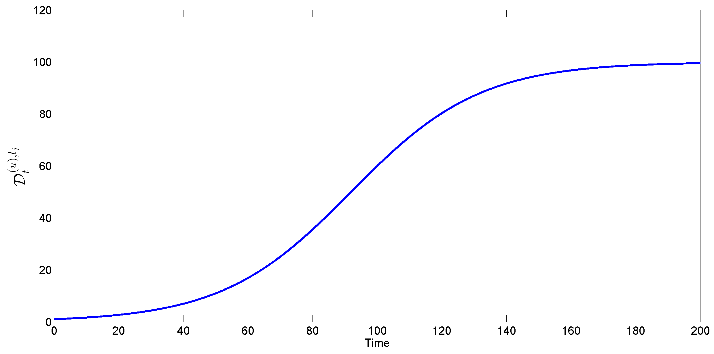
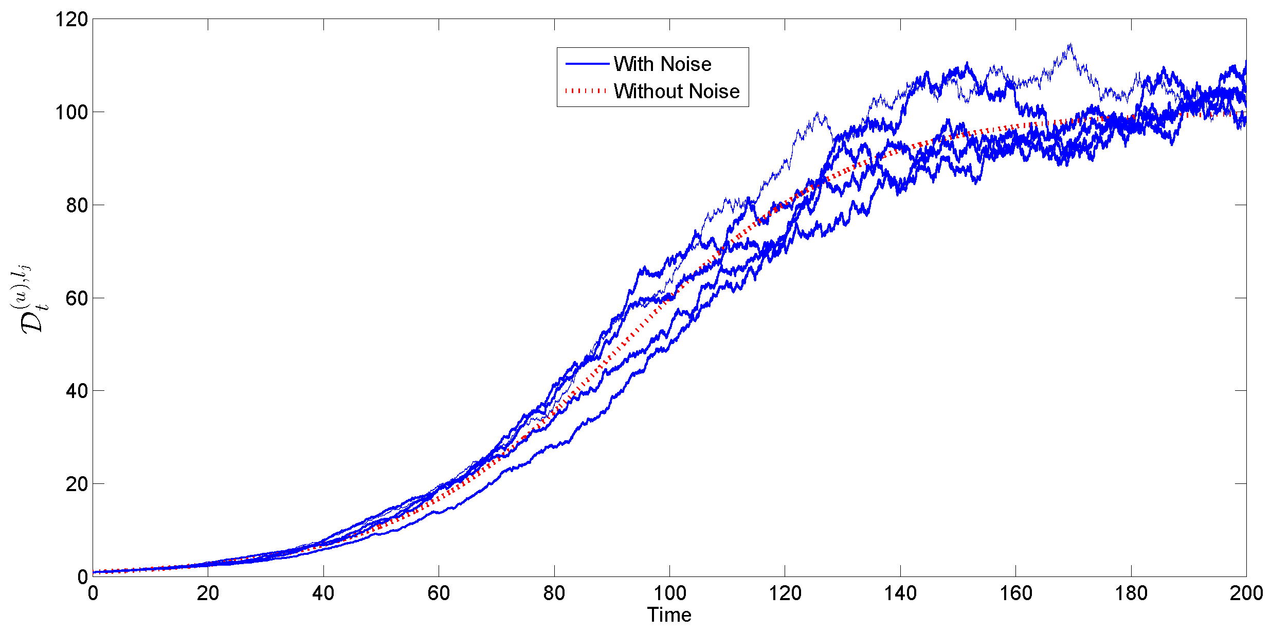
4.1.3. Stochastic Logistic Replenishment

The standard logistic resource model, widely used in multi-robot systems (see e.g., [2,47]), can be described by:
d D t ( u ) , l j d t = λ D t ( u ) , l j 1 D t ( u ) , l j K
where λ is the unconstrained growth rate and K is the maximum carrying capacity of the environment. In other words, D t ( u ) , l j follows the standard logistic growth model with self-limiting growth. Because Equation (3) is deterministic, the entire resource evolution can be conveniently computed in advance, assuming that the parameters λ and K in this model are known a priori. Choosing λ = 0 . 04 , K = 100 and the minimum population bound D 0 ( u ) , l j = 1 , the resource evolution based on this model is simulated in Figure 1.
Figure 1. Resource evolution of the logistic model in Equation (3).
Robotics 04 00365 g001
However, in reality, there is often uncertainty in the resource model due to the fact that resource replenishment is usually not an isolated process, but rather, is affected by external/environmental inputs, too, which may be stochastic in nature. To take into account such environmental stochasticities, as well as density-dependent resource replenishment, we adopt the stochastic logistic model [48]:
d D t ( u ) , l j d t = λ D t ( u ) , l j 1 D t ( u ) , l j K + σ e D t ( u ) , l j d W e ( t )
where σ e is the intensity of the growth rate fluctuation, d W e ( t ) is delta-autocorrelated white noise, i.e., mean zero and randomly changing sign within any short time interval, and “∘” denotes the “Stratonovich calculus”. The explanation of Stratonovich calculus will be given later.
The process with increments d W e ( t ) representing the noise in the above stochastic logistic model is the Brownian motion. For any 0 < t 1 < t 2 < t 3 and h > 0 , W e ( t ) has the following properties:
  • Independent increments: W e ( t 3 ) W e ( t 2 ) is independent of W e ( t 2 ) W e ( t 1 ) ;
  • Stationary increments: ( W e ( t 2 + h ) W e ( t 1 + h ) ) ( W e ( t 2 ) W e ( t 1 ) ) ;
  • Gaussian increments: ( W e ( t 2 ) W e ( t 1 ) ) N ( 0 , t 2 t 1 ) .
This means that W e ( t + h ) W e ( t ) is independent of the history of W e ( s ) , s < t . Although Brownian motion has continuous paths, the above properties imply that it is nowhere differentiable, and hence, d W e ( t ) d t does not exist.
In order to use the model Equation (4) to compute D t ( u ) , l j , the resource at time t, we need to express the differential equation into a different form. First, we take integrals on both sides of Equation (4) to obtain:
D t ( u ) , l j = D 0 ( u ) , l j + 0 t ( λ D s ( u ) , l j 1 D s ( u ) , l j K ) d s + 0 t σ e D s ( u ) , l j d W e ( s )
To deal with the last term of Equation (5), we first consider the following Riemann–Stieltjes integral:
0 t σ e D s ( u ) , l j d W e ( s ) = lim n j = 1 n σ e D τ j ( u ) , l j ( W e ( t j + 1 ) W e ( t j ) )
If W e ( t ) is a smooth function, the above limit converges to a unique value regardless of whether τ j is chosen in the interval [ t j , t j + 1 ] . However, since W e ( t ) is not smooth in the above stochastic logistic model, the limit will depend on the value of τ j . Thus, different choices lead to different stochastic calculi: τ j = t j leads to “Ito calculus”, denoted by 0 t σ e D s ( u ) , l j · d W e ( s ) , and τ j = t j + t j + 1 2 leads to “Stratonovich calculus”, denoted by 0 t σ e D s ( u ) , l j d W e ( s ) . Thus, we have the following relationship between “Stratonovich calculus” and “Ito calculus”:
0 t σ e D s ( u ) , l j d W e ( s ) = 0 t 1 2 σ e 2 D s ( u ) , l j d s + 0 t σ e D s ( u ) , l j · d W e ( s )
Substituting Equation (7) into Equation (5), we obtain:
D t ( u ) , l j = D 0 ( u ) , l j + 0 t λ D s ( u ) , l j ( 1 D s ( u ) , l j K ) + 1 2 σ e 2 D s ( u ) , l j d s + 0 t σ e D s ( u ) , l j · d W e ( s )
where the “Ito calculus” integral term can be expressed as:
0 t σ e D s ( u ) , l j · d W e ( s ) = lim n q = 1 n σ e v j , s q ( W e ( s q + 1 ) W e ( s q ) )
From Equation (8), we employ Euler’s method to obtain D ¯ t ( u ) , l j , a discretized approximation of the solution D t ( u ) , l j between t and t + Δ t , as follows:
D ¯ t + Δ t ( u ) , l j = D ¯ t ( u ) , l j + λ D ¯ t ( u ) , l j ( 1 D ¯ t ( u ) , l j K ) + 1 2 σ e 2 D ¯ t ( u ) , l j Δ t + σ e D ¯ t ( u ) , l j ( W e ( t + Δ t ) W e ( t ) )
Thus, from Equation (10), we are able to compute an estimate of the resource at the next time step. Note that the distribution of W e ( t + Δ t ) W e ( t ) can be simulated by generating a standard Gaussian distribution N ( 0 , 1 ) multiplied by Δ t .
As an example, let the parameters be selected as σ e = 0 . 02 , λ = 0 . 04 , K = 100 and D 0 ( u ) , l j = 1 . Using Monte Carlo simulation with N = 100 scenarios, we generated several iterations of the approximated resource evolution D t ( u ) , l j , as shown in Figure 2. The red dotted curve shows the resource evolution without noise.
From the figure, there exist obviously different resources at some time points for the different iteration process. This implies that the resource becomes difficult to predict accurately with the stochastic environmental noise.
Figure 2. Replenishment of resources at a location that follows the stochastic logistic model [1].
Robotics 04 00365 g002

4.2. Applying Resource Replenishment Models to Item Delivery

The three resource replenishment models we contribute above were designed for the multi-robot foraging problem, but are also applicable to the multi-robot item delivery problem. Specifically, since the models assume that demands are generated at locations independently, a uniform distribution of locations can be created in the space (i.e., every fixed interval spanning L ). After doing so, the replenishment models can be used at each discrete location.
Among the three replenishment models, we believe that the Poisson model suits the multi-robot item delivery problem best:
  • Having no upper limit suits the multi-robot item delivery problem, since guests may typically request an unlimited number of refreshments;
  • The Poisson distribution is suitable for modeling how demands may be created over time.
However, the assumption that replenishment is independent of location may not be entirely valid: in a cocktail party, people tend to congregate in groups, so a demand generated at a location l j has a high correlation with a nearby location l k . In this article, we will not address such dependencies, and we leave creating a better demand generation model to future work.

5. Distributed Algorithms for Item Delivery

In this section, we first present distributed algorithms that solve the multi-robot foraging problem. Next, we discuss how these algorithms apply to the multi-robot item delivery problem.

5.1. Multi-Robot Foraging Algorithms

We now describe five distributed foraging algorithms, three (greedy rate, adaptive sleep and adaptive sleep with target change) of which were previously introduced in [1]. The other algorithms are listed as baselines and comparisons to the three from [1].

5.1.1. Random

The baseline algorithm for an agent is to randomly select a location to visit. When the agent arrives at its desired location, it randomly selects the next location to visit. In particular, the agent has a p v probability of visiting another location if y i < c i and always heads home if its payload is full, i.e., y i = c i :
Random ( r i ) = rand ( l 1 , , l m ) if y i = 0 rand ( l 1 , , l m ) if y i < c i with probability p v l 0 otherwise
where l 0 is the home location.
One key characteristic of the random algorithm in the multi-robot foraging problem with the Bernoulli model of resources is that the probability of a robot r i completely filling up its capacity increases as the number of locations | L | increases:
Theorem 1 If the resource replenishes following the Bernoulli model of replenishment (Section 4.1.1), then as | L | , P ( D t ( s ) , l j > c i y i ) 1 .
Proof. Sketch: as | L | increases, the average time between visits of any location l j increases. Since D t ( u ) , l j (the number of unsatisfied demands at location l j ) follows the Bernoulli replenishment model, there is no upper limit of the number of resources available, and hence, P ( D t ( u ) , l j > c i y i ) increases.
In our experiments, we investigate the relationship of the maximum capacity c i when all agents a i employ the Random algorithm.

5.1.2. Best Static Loop

The second algorithm finds the best static loop for a robot r i , i.e., r i considers a cycle Γ i = ( l 0 , l i 1 , , l i R , l 0 ) , such that:
l i α l i β 1 α , β R , α β
V Γ i = max ( c i , l i α Γ i E ( | D t Γ i ( u ) , l i α | ) ) , where
t Γ i = l i α , l i α + 1 Γ i t ( r i , l i α , l i α + 1 )
In particular, since we are interested in continuous foraging (and the resources replenish themselves over time), the robot seeks to maximize the rate of foraging:
Γ i * = argmax Γ i V Γ i t Γ i
Equation (12) considers E ( | D t Γ i ( u ) , l i α | ) ) , the expected number of resources at a location after t Γ i time steps, where t Γ i is the number of time steps to complete the loop. Since the number of resources at every location is initialized to zero when t = 0 and, on expectation, the robot should completely forage all available resources at locations in its loop, E ( | D t Γ i ( u ) , l i α | ) ) provides an estimate of how many resources will be replenished every loop r i makes.
Hence, the goal of the best static loop algorithm is to forage c i resources every loop, while minimizing the total time of traveling the loop. The primary benefit of the best static loop algorithm is that the agent does not need to replan at any time, and on expectation, it completely fills up its capacity. However, the drawback is that since the robot does not replan, if a location has fewer resources than expected, the agent will return to the home location l 0 with some capacity remaining (assuming all other locations have the expected number of resources). Another related drawback is that unvisited locations will accumulate resources that are never foraged by the robot. Further, Γ i * is computationally expensive to find, since all possible loops have to be considered.
Due to the drawbacks listed above, we will not evaluate the performance of best static loop in our experiments later.

5.1.3. Greedy Rate

The random algorithm above has the benefit that it probabilistically visits all locations, and given enough time, a location that replenishes resources following the Bernoulli or Poisson models will have more resources than the robot’s capacity. However, the random algorithm does not make use of the robot r i ’s model of resource D ^ t , i ( u ) to select which location to visit.
The best static loop algorithm has the benefit of maximizing the foraging rate, i.e., the rate of moving resources from the locations to the home location, given a static loop. The algorithm has the drawback of being computationally expensive, as well as being “stuck” on a pre-defined loop.
The greedy rate algorithm [1] that we contribute aims to capture the benefits of random and best static loop, while minimizing the drawbacks. Algorithm 1 shows the pseudocode of the greedy rate algorithm. The key idea of the greedy rate algorithm is that the robot only selects its next destination (similar to random), but it selects the destination by greedily optimizing the expected foraging rate (similar to best static loop). Upon reaching its destination, the greedy rate algorithm replans and selects the next destination for the robot, which allows the robot to use updated information from its observations, as well as information from the other robots in the team.
Lines 2–4 of Algorithm 1 are the base case: if r i is no longer able to forage any more resources, i.e., its payload y i equals its capacity, then r i heads to the home location l 0 to drop off all of its resources.
Lines 6–7 compute the current foraging rate of r i if r i heads home. It does so by dividing its current payload y i by the time taken to travel from its current location l α to the home location l 0 . This foraging rate serves as a baseline for r i to decide if visiting a new location l β is worthwhile.
Line 10 iterates through the robots that are also heading to l β and sums up their remaining capacity as e β . The purpose of doing so is to discount the expected number of resources at l β by e β , since those resources will be foraged by other robots. Hence, Line 11 computes the number of resources that are expected to be available to be foraged by r i when it visits l β at time step t + t ( r i , l α , l β ) .
Line 12 computes the expected foraging rate of r i if it visits l β and heads back to l 0 , and Lines 13–16 greedily select the best location l β .
Robotics 04 00365 i001
Overall, the greedy rate algorithm seeks to improve a robot r i ’s marginal foraging rate, by greedily considering the next best location to visit. It computes the expected foraging rate by using the robot’s estimate D ^ t + t ( r i , l α , l β ) , i ( u ) . Hence, the algorithm performs better if the robot’s model is more accurate, e.g., by receiving more information from its teammates. The greedy rate algorithm coordinates with its teammates through “ear-marking” (Line 10), where robots do not consider resources that will be foraged by their teammates that are also en-route to the same location. We chose ear-marking for coordination, because it requires limited communication bandwidth and computation (useful for low-cost foraging robots that typically have limited processing power).
We investigate the performance of the greedy rate algorithm and how it performs compared to the random algorithm, over a variety of robot team sizes and capacities, in our Experimental Section. The greedy rate algorithm is an improvement over the continuous sweeping algorithm [3], which we also compare against in the experiments. Next, we present our algorithms for multi-robot foraging when resources replenish following the stochastic logistic model.

5.1.4. Adaptive Sleep

We first contributed the adaptive sleep algorithm in [1]. The adaptive sleep algorithm is inspired from an algorithm in sustainable foraging [2], and we discuss the similarities and differences between the two algorithms later.
Algorithm 2 shows the pseudocode of our adaptive sleep algorithm. The overall idea of our adaptive sleep algorithm is that it is designed for the stochastic logistic replenishment model, and each foraging robot picks a unique foraging location by communicating its decisions initially. Once a robot r i has selected its foraging location l α , r i sleeps (stays at the home location l 0 ) until l α has K α 2 resources according to r i ’s model, where K α is the maximum number of resources at l α . In particular, r i takes into account the travel time t ( r i , l 0 , l α ) to l α in its computation.
Robotics 04 00365 i002
The robot r i waits until l α has K α 2 resources, because in the logistic distribution, the change in resources is highest at K α 2 . As such, by foraging at that amount, the location will replenish its resources at the fastest rate. However, since the capacity of r i may be greater than one, r i sleeps until there are K α 2 + c i resources, where c i is r i ’s capacity. When a robot is sleeping, it can shut off its motors and most processing, but continues actively listening and processing messages from its teammates, then it will “wake up” earlier as a result of the messages.
The robots select their assigned location by two steps iteratively. In the first step, each robot r i randomly selects a location l α . The robots then broadcast their choices to nearby teammates. If two robots r i and r j select the same location, then the robot with the higher id, e.g., r j , repeats the first step again. The assumption is that the number of locations | L | is greater or equal to the number of robots n. If the | L | < n , then an additional step occurs prior to the location assignment, where n | L | robots stay permanently “asleep”.
A key difference between our adaptive sleep algorithm and the sustainable foraging algorithm [2] is that robots running our adaptive sleep algorithm sleep at the home location until there are K α 2 resources in their model. As such, if additional information is received (from another robot on the team), informing that there are more resources than expected (since the resources replenish stochastically), then the robot will awaken early to forage it. Furthermore, if there are less resources than expected, the robot will sleep for a longer time.
In contrast, the sustainable foraging algorithm uses a proportional controller to determine how long to sleep. A robot adjusts its sleeping time based on the observations of the number of resources when it forages the location. As such, the robot is unable to make use of any information gathered by its teammates. Furthermore, the sustainable foraging algorithm does not handle stochasticity in the replenishment, so the proportional gain may fluctuate and not converge effectively based on the observations.
A benefit of the sustainable foraging algorithm is that it prevents locations from being over-foraged and causing a population collapse, where there are insufficient resources to replenish the population (e.g., if there is only one fish left in a pond, the number of fish cannot replenish). We do not directly model population collapses, but we ensure that the foraging robots always leave a minimum number of resources at the location (e.g., if there are x resources, but a minimum of y resources are required to prevent over-collapse, then the robot only forages x y resources).

5.1.5. Adaptive Sleep with Target Change

The adaptive sleep with target change algorithm [1], as its name suggests, is an extension of the adaptive sleep algorithm. In the adaptive sleep algorithm, each robot r i is assigned a unique location l α . However, if | L | > n , i.e., there are more locations than robots, then some locations will never be foraged.
In particular, these locations will eventually reach their maximum population size and stay there. To take advantage of these unassigned locations, the adaptive sleep with target change algorithm makes use of the “sleep” time of the robots. In particular, if a robot r i anticipates that it will sleep at the home location for k time steps (based on its model of its assigned location l α ) and there is another location l β that is close enough, i.e., a round-trip time of less than k time steps, then r i will visit l β , as well.
These extra visits are selected randomly over the possible locations within k time steps, and the key idea is to forage extra resources (compared to the adaptive sleep algorithm). However, since the robots do not coordinate over these “target change” visits, it is possible that two robots visit the same location l β (or visit at a small time interval), so it brings l β ’s resources below the ideal K β 2 .
We analyze the performance of the adaptive sleep and adaptive sleep with target change algorithms later in the Experimental Section, but in general, we feel that as long as n | L | , the probability that two robots will visit the same location is small. In addition, if two robots visit the same location within a short time frame, there is also a high probability that no robots visit that location for some time, so the resources will replenish to a high amount before another robot visits it.

5.2. Adapting the Foraging Algorithms for Item Delivery

The algorithms that we contributed in the previous section were designed for the multi-robot foraging problem. However, they are also applicable to the multi-robot item delivery problem.
In particular, the foraging algorithms assume that there is a discrete set of locations L where the robots select their destinations. In the multi-robot item delivery problem, demands can be created anywhere in the location space. As such, to apply the foraging algorithms to the item delivery problem, “foraging locations” can be added in a grid-like fashion through the location space. For example, if the location is a 100 m × 100 m space, then locations can be created every 10 m, so that there are 100 discrete locations.
After creating such pseudo foraging locations, the multi-robot foraging locations can be run with minor modifications, i.e., when a robot arrives at a location, it may have to travel a small distance to serve the actual demand. Furthermore, demands within a certain radius have to be consolidated into a pseudo foraging location for the models to be updated.
In addition, we modified the greedy rate algorithm slightly to form the greedy rate while ignoring capacity (GRIC) algorithm, as shown in Algorithm 3.
Robotics 04 00365 i003
The main difference between Algorithms 1 and 3 is in Line 11. The GRIC algorithm does not take the maximum capacity of the robot into account when computing the potential rate. We made this change so that the robots would visit locations further from the home location over time. Otherwise, the robots would tend to only visit locations close to home, since they would be able to fully fill their capacity (or so they assume from the model), while minimizing the distance traveled. By visiting the far-away locations from time to time, the robot is able to increase its delivery rate, since these locations will have a higher number of accumulated demands.
We will analyze the performance of the multi-robot foraging algorithms in such scenarios for item delivery later in the Experimental Section.

6. Maintaining a Model of the World

In this section, we describe how the multi-robot team maintains a model of the world, i.e., the locations and details of demands for item delivery, as well as the locations, payloads and current destination of the robots.
The algorithms we described in the previous section are completely distributed, and similarly, the robots in the multi-robot team maintain individual world models. However, through communication, the robots synchronize their information, so that they actually have a shared world model.
We first describe how the demands are modeled and then discuss how the robots communicate to synchronize their world model and how it behaves when there are errors in communication and/or latency in messages.

6.1. Modeling Demands at Locations

In Section 4, we described how the demands are modeled per time step. In particular, we discussed three resource replenishment models: Bernoulli, Poisson and stochastic logistic.
In each robot’s world model, it maintains a model of the number of demands in each location. We previously discussed how the locations are finite in number in the multi-robot foraging problem and how the approach is extended for the multi-robot item delivery problem. As such, the robot’s world model maintains a discrete number of locations and models the number of demands at each location.
Recall at D ^ t , i ( u ) , l j is robot r i ’s model of D t ( u ) , l j , the number of unsatisfied demands at location l j at time t. At the start of the run, i.e., t = 0 , the robot assumes that D ^ 0 , i ( u ) , l j = D 0 ( u ) , l j = 0 for the Bernoulli and Poisson replenishment models and D ^ 0 , i ( u ) , l j = D 0 ( u ) , l j = K j 2 for the stochastic logistic replenishment model, where K j is the maximum population of location l j .
Each replenishment model has associated parameters, and the robots are not aware of the true parameters of the models:
  • Bernoulli replenishment: p j is not known, and the robots use a preset value p ^ for all locations;
  • Poisson replenishment: λ j is not known, and the robots use a preset value λ ^ for all locations;
  • Stochastic logistic replenishment: The unconstrained population growth rate r j and maximum population K j is known, but the intensity of growth rate fluctuation σ e is not known. The robots assume that σ ^ e = 0 , i.e., there is no noise in the growth rate.
Hence, given the initial estimate D ^ 0 , i ( u ) , l j , and the estimated model parameters (e.g., p ^ for the Bernoulli replenishment model), the robot r i can predict the number of resources at l j for any future time t > 0 . During execution, the robot uses these estimates D ^ t , i ( u ) , l j to make decisions as to which locations to visit, e.g., Line 11 of Algorithm 1 and Line 4 of Algorithm 2.
When a robot makes an observation, i.e., when the distance between the robot and a location l j is less than or equal to o i , the observational range of the robot, the robot is able to observe the number of demands at l j . Suppose that robot r i observes location l j at time t. When that occurs, the robot r i updates its model, such that D ^ t , i ( u ) , l j = O j , where O j is the number of observed demands at l j . Note that O j may not be equal to D t ( u ) , l j if there is noise in observations, e.g., the robots are not able to perceive the number of demands exactly.

6.2. Synchronizing the Shared World Model

In the previous subsection, we discussed how each robot maintains its own models of the demands at the locations. In this subsection, we discuss how the robots communicate and synchronize their world models.
We base our shared world model architecture from the CMurfs (Carnegie Mellon United Robots for Soccer) RoboCup world model, which was described in detail in [49,50]. The key idea of the shared world model is that the robots individually maintain a copy of the world model, but communicate their individual states periodically. Upon receiving packets from a teammate r j , the robot r i ’s world model is updated with regards to r j ’s information.
In particular, for the multi-robot item delivery problem, each robot r i ’s world model keeps track of:
  • The global position of every robot in the multi-robot team;
  • l j L , D ^ t , i l j , a model of the number of demands (satisfied and unsatisfied) at location l j at time t;
  • For each robot r i , which demands have been assigned to r i ;
  • The current destination of every robot r i .
For the description below, we will use the perspective of a single robot r i on the team and how its world model is updated and synchronized with information from its teammates.
r i tracks its global position through its localization system and maintains demand models D ^ t , i l j for each location l j , as described in the previous subsection. When r i makes new observations of the number of demands at locations, it updates its demand models D ^ t , i l j .
Every time step, the robot r i broadcasts information to teammates that are in communication range C. In particular, r i broadcasts:
  • r i ’s global position;
  • r i ’s observations of demands at locations;
  • r i ’s assigned demands;
  • r i ’s current destination.
Note that the four components of r i ’s broadcast message match the four components of the world model by design. Hence, if all of the robots broadcast these messages, a union of their information forms the complete world model of the multi-robot team.
Hence, if there is no limit to the communication range and no errors in transmission, then the world models of the robots will be completely synchronized at all times. However, in practice, it is rarely the case that communication is perfect. Robots may go in and out of communication range, and broadcast packets may not be received in a timely fashion.
In our shared world model paradigm, we use UDP to send the broadcast packets, because we prefer information to arrive on time, or not at all, compared to receiving old information via TCP. Timely information is more useful, because the robots’ information typically does not change every time step, so losing some packets does not have large effects on the shared world model. Further, because any packet that is received will be timely, even if robot r i ’s model is outdated with regards to r j ’s information, it will be fully up-to-date the moment communication between r i and r j is restored, i.e., a packet from r j is received by r i .
To go one step further and to handle the limited communication range C, robots may also transmit extra information in their broadcast packet, namely information received from teammate robots; in this way, a robot r i may receive information from r k , even if r i and r k are not within communication range, by using another robot r j to pass on its latest information from r k . However, doing so involves a caveat that third-party information must be time-stamped, so that the receiving robot can discard old information, e.g., if two robots r j and r m send information about r k , r i should only use the latest version of the information. However, we do not consider this case in this article and leave it for future work.
Thus, by communication via broadcast packets, the robots in the multi-robot team are able to maintain a synchronized world model and plan effectively to solve the multi-robot item delivery problem.

7. Experiments and Results

In this section, we describe our comprehensive experiments to evaluate the efficacy of our distributed multi-robot algorithms and shared world model. We first describe experiments in the multi-robot foraging problem and next present results in the multi-robot item delivery problem.

7.1. Multi-Robot Foraging Experiments

As discussed in Section 4, we considered three resource replenishment models: Bernoulli, Poisson and stochastic logistic. We evaluated the greedy rate (GR) algorithm in the Bernoulli and Poisson replenishment models, against the benchmark of random (R) algorithm and continuous area sweeping (CAS) [3]. Similarly, we evaluated the adaptive sleep (AS) and adaptive sleep with target change (ASTC) algorithms in the stochastic logistic replenishment model, against the random (R) and sustainable foraging (SF) [2] algorithms.

7.1.1. Experimental Setup

We created a 2D simulator in Java, which we first used in [1]. In the simulation, a discrete number of locations are created following the replenishment models, and the robots start from a home location to forage the resources.
For each of the replenishment models, we used the following parameters:
  • Space of the world: N × N ;
  • Home location: center of the world;
  • Number of locations: 20, uniformly distributed in the world;
  • Number of robots: 1–10;
  • Capacity of each robot: 1–20;
  • Maximum speed of each robot: N 5 ;
  • Length of simulation: 1000 time steps;
  • Full communication between robots to share the world model, i.e., perfect communicate with no limits on range and no errors in communication.
One key difference between our experiments in this article, compared to our previous work in [1], is that we consider the robots having a shared world model in this article, whereas in [1], we only considered that the robots shared their destinations within a small communication range and did not share additional information; instead, they relied on an information-gathering agent to discover and share information among the multi-robot team. In this article, all robots share their information with the entire team, and hence, the information-gathering agent is not required.
Furthermore, the size of the world, N × N , is arbitrary, since the speed of the robot is set to N 5 .
The parameters for the robots’ model of the demands were set depending on the replenishment model:
  • For the Bernoulli replenishment model, p ^ = 0 . 3 ;
  • For the Poisson replenishment model, λ ^ = 0 . 5 ;
  • For the stochastic logistic replenishment model, σ ^ e = 0 .
When we created the locations, we sampled the true model parameters from normal distributions:
  • Bernoulli model: p j N ( 0 . 3 , 0 . 15 2 ) ;
  • Poisson model: λ j N ( 0 . 5 , 0 . 4 2 ) ;
  • Stochastic logistic model: σ e 0 . 04 , 0 . 08 , 0 . 12 , 0 . 16 , 0 . 20 .
We chose these values so that the locations have a spread of true parameter values and so that the resource generation was at a rate such that with 20 robots and 10 capacity each, the random algorithm was able to forage almost all resources.
For each set of parameters, we ran 20 trials in simulation.

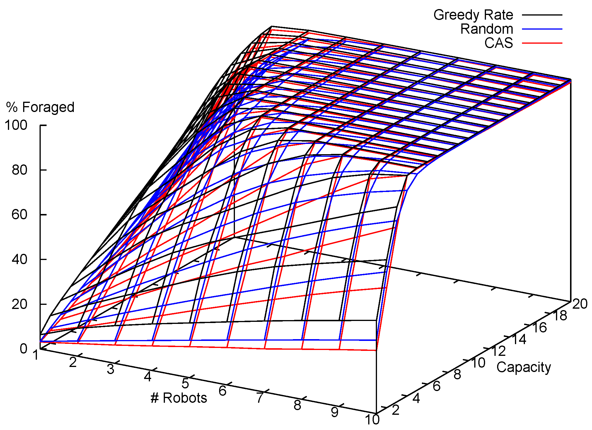
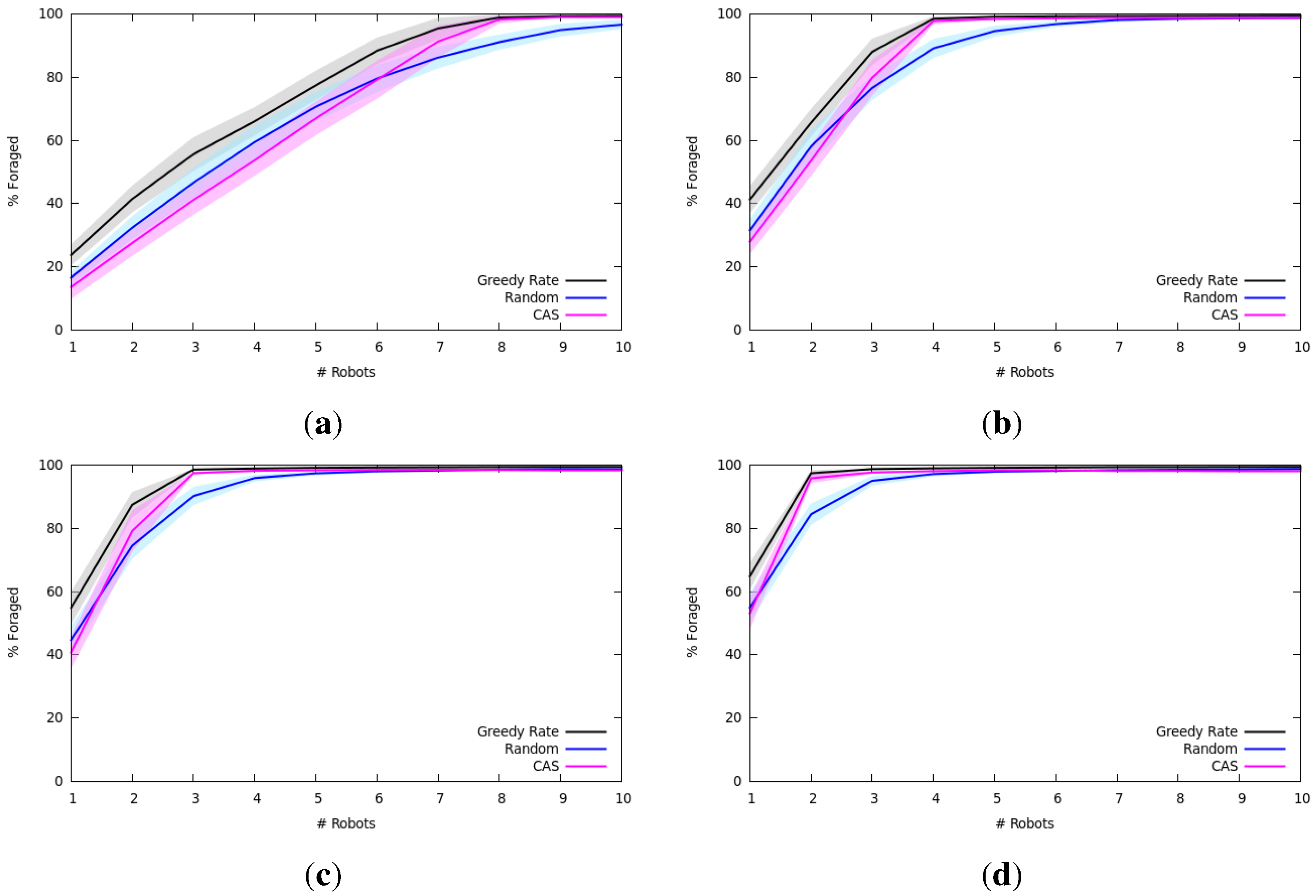
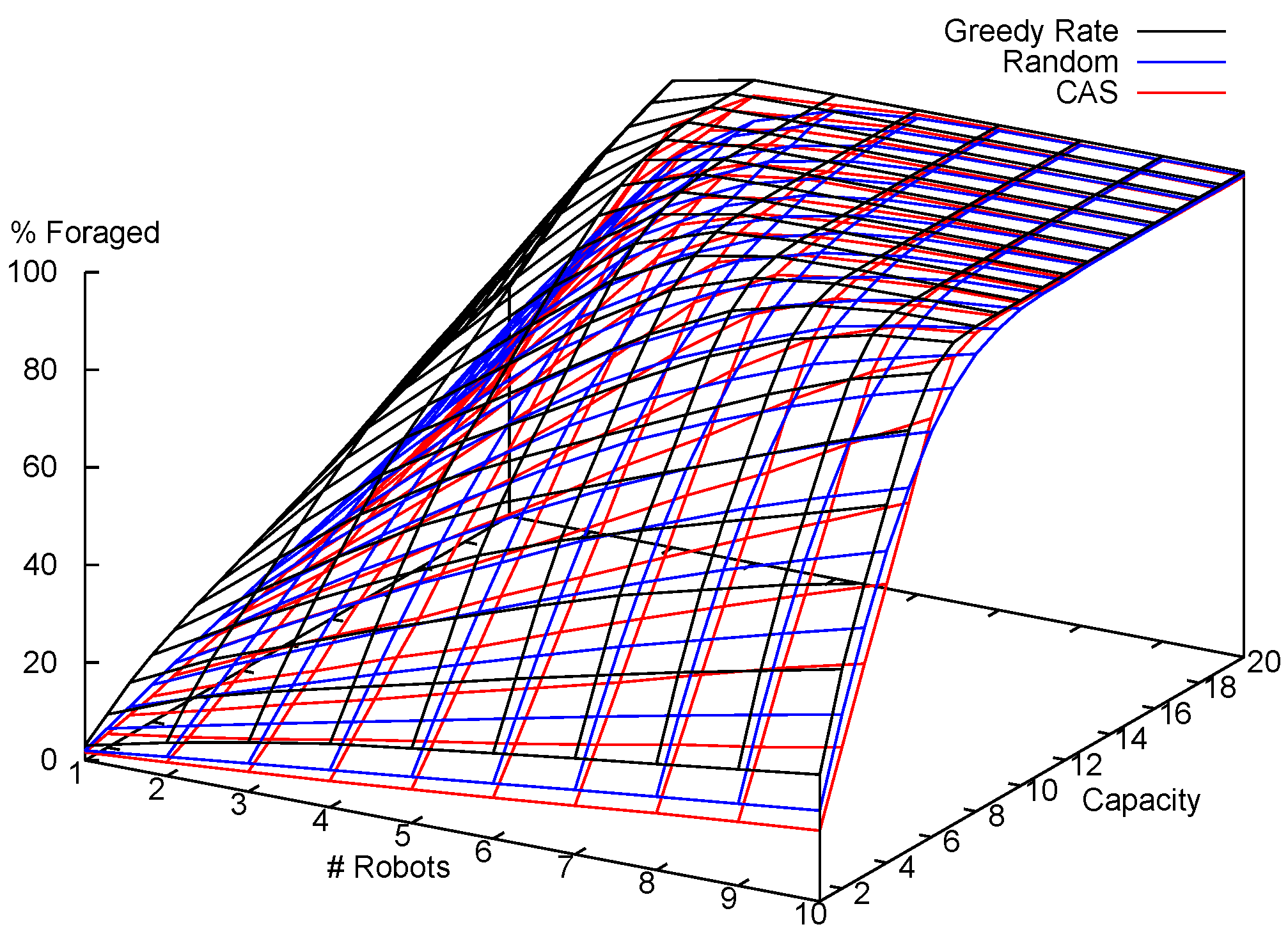
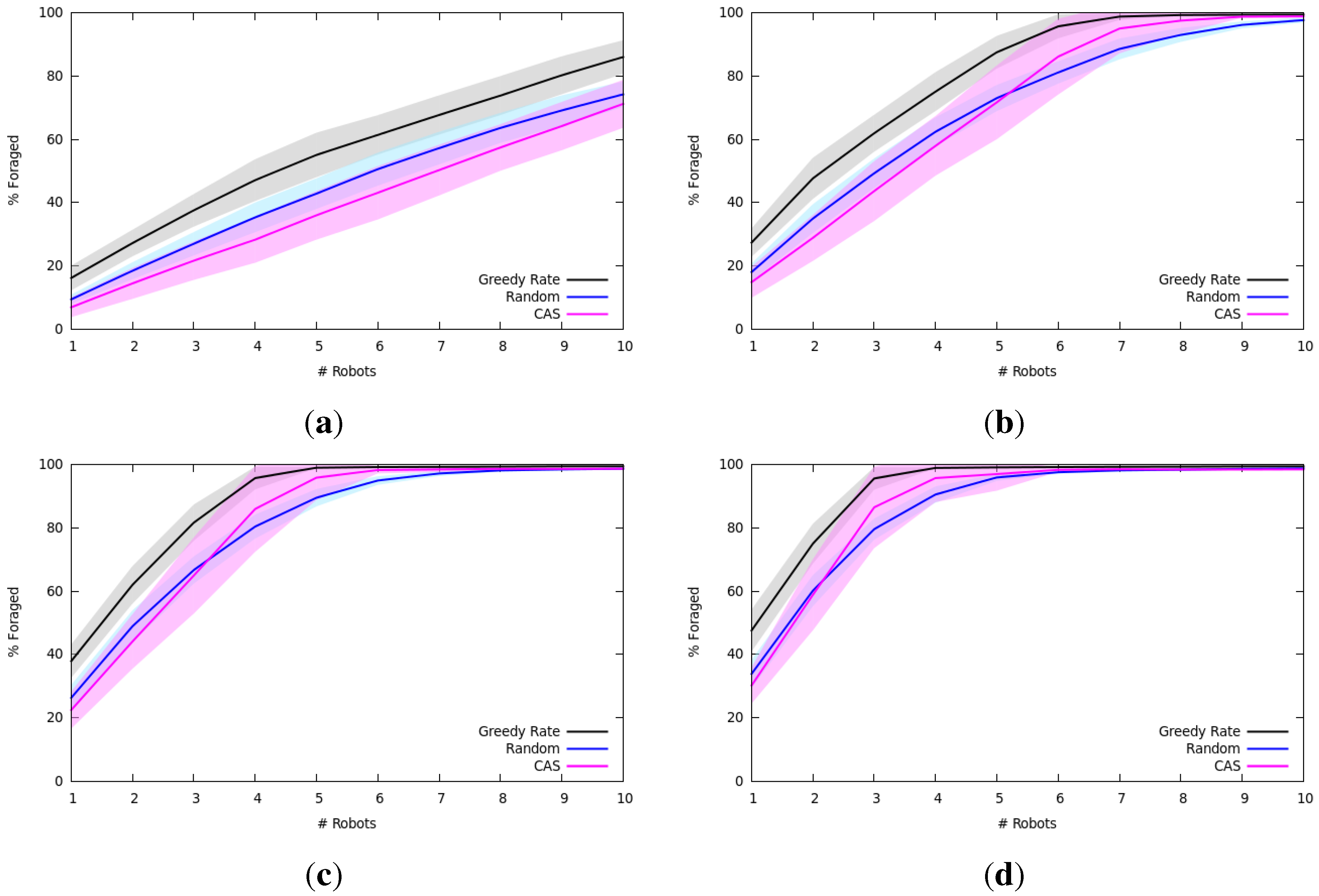
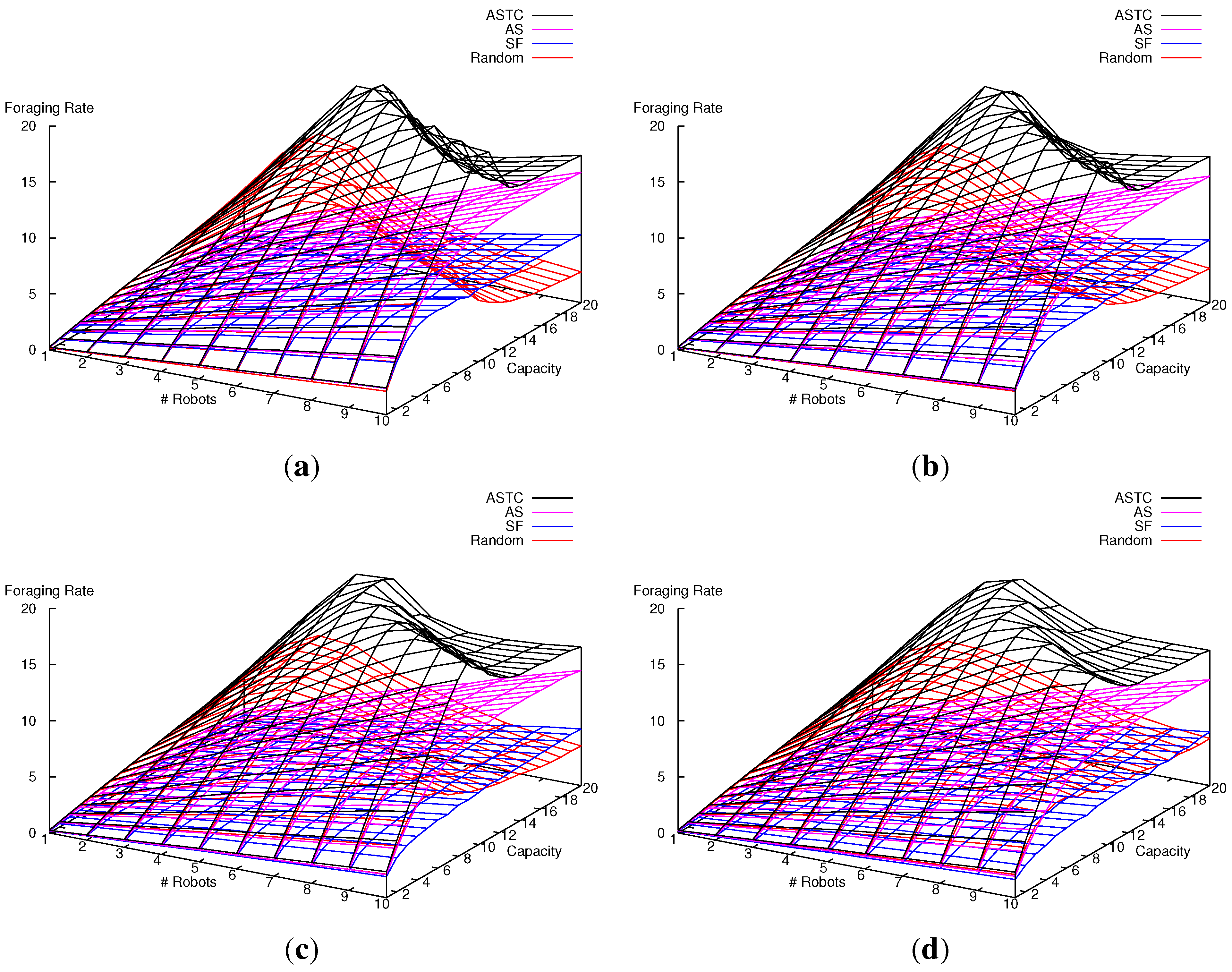
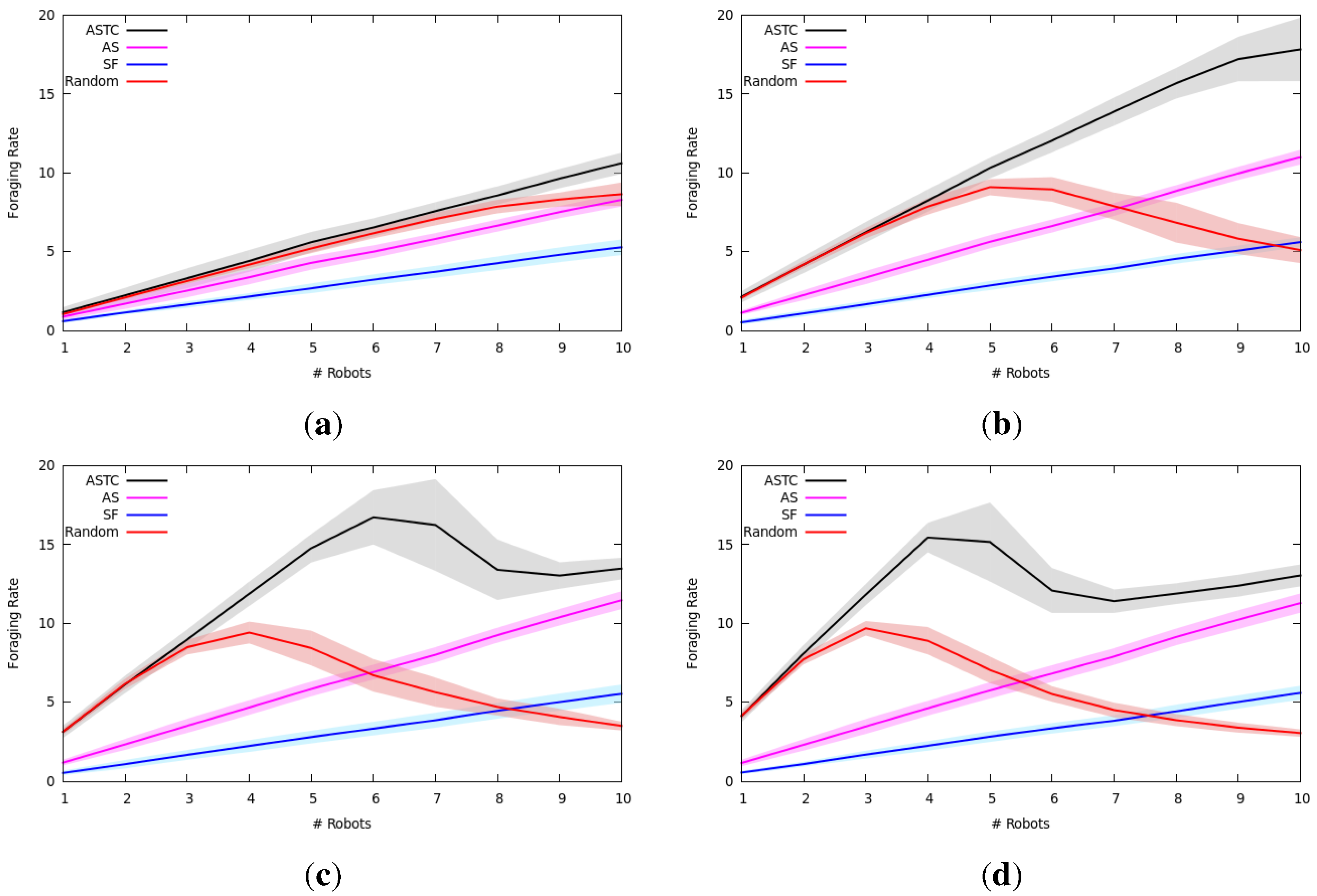
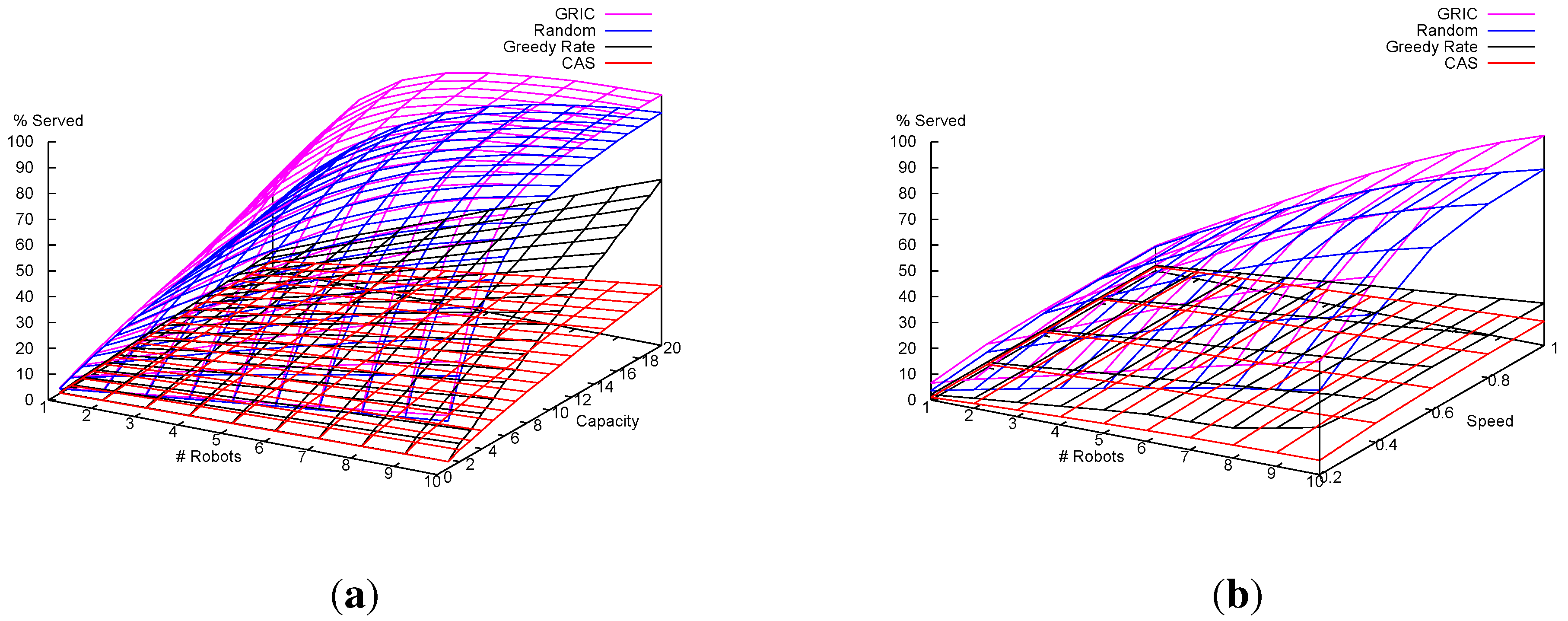
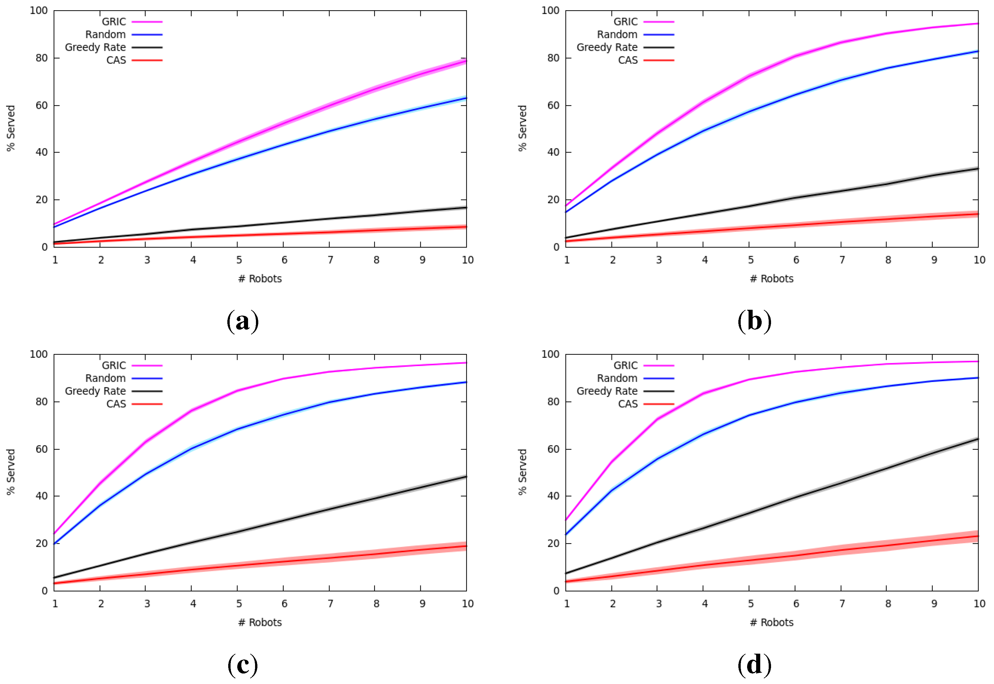
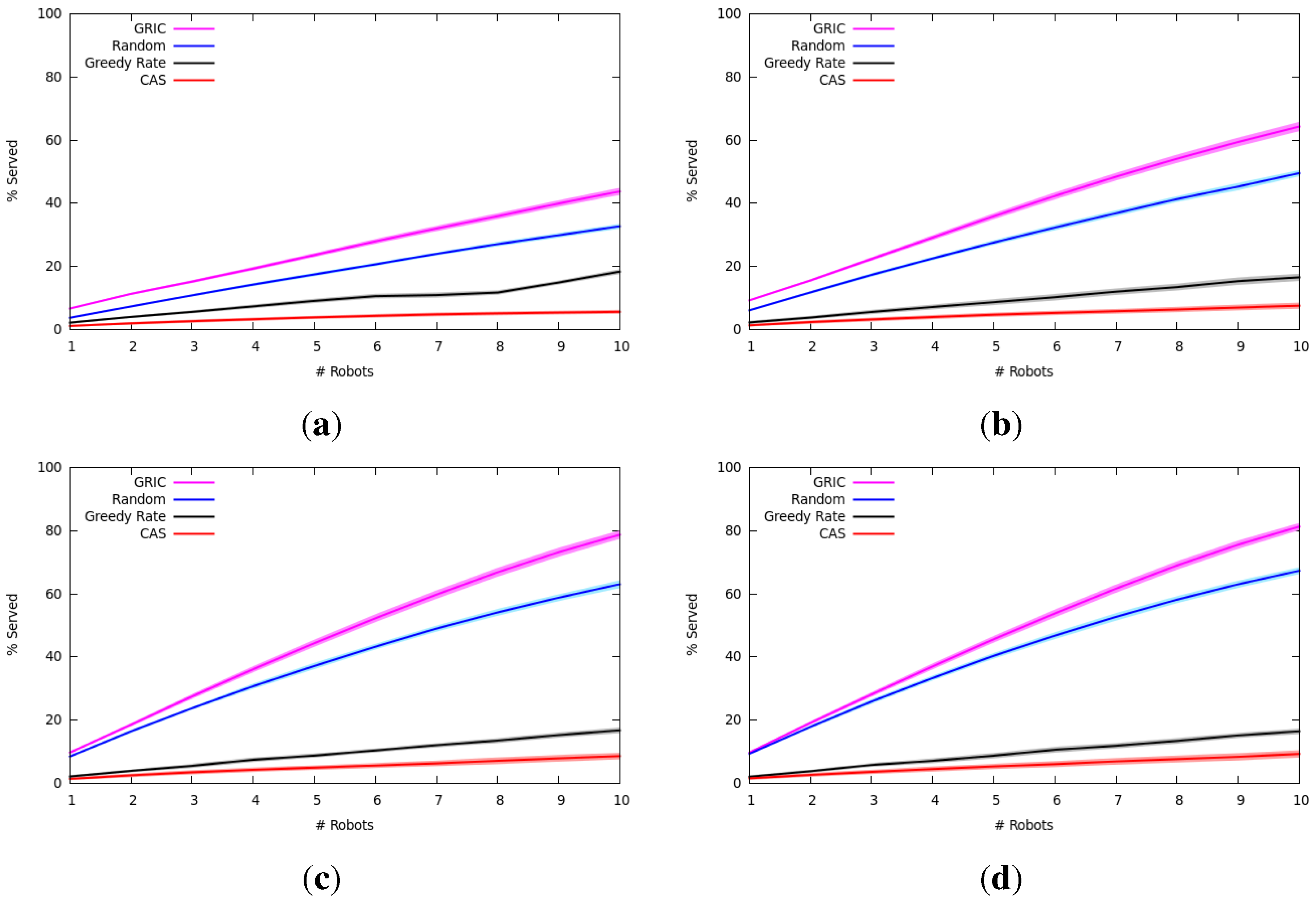
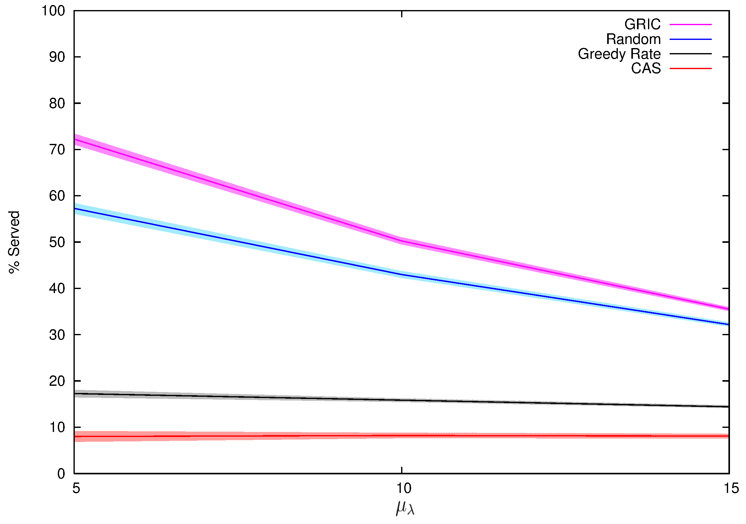
7.1.2. Results and Analysis

Figure 3 shows the results of the experiments with the Bernoulli replenishment models, and Figure 4 shows 2D slices of Figure 3, where the shaded regions indicate the standard deviations of the results. We performed two-tailed Student’s t-tests for the graphs in Figure 4 and found that greedy rate outperformed CAS with p = ( 4 × 10 37 , 3 × 10 18 , 1 × 10 14 , 3 × 10 15 ) for capacities = ( 5 , 10 , 15 , 20 ) , respectively. Similarly, greedy rate outperformed random with p = ( 1 × 10 72 , 6 × 10 35 , 2 × 10 25 , 8 × 10 22 ) , respectively.
Figure 5 and Figure 6 show the results of the experiments with the Poisson replenishment model in 3D and 2D, respectively. We also performed two-tailed Student’s t-tests for the graphs in Figure 6 and found that greedy rate outperformed CAS with p = ( 4 × 10 66 , 7 × 10 28 , 1 × 10 17 , 3 × 10 14 ) for capacities = ( 5 , 10 , 15 , 20 ) , respectively. Similarly, greedy rate outperformed random with p = ( 3 × 10 95 , 4 × 10 67 , 4 × 10 39 , 1 × 10 29 ) , respectively.
Figure 3. Foraging rate (as a % of total resources generated) using the Bernoulli replenishment model.
Robotics 04 00365 g003
Figure 4. Foraging rate (as a % of total resources generated) using the Bernoulli replenishment model, i.e., 2D slices of Figure 3. The shaded regions indicate the standard deviations of the results. (a) Capacity = 5 ; (b) capacity = 10 ; (c) capacity = 15 ; (d) capacity = 20 .
Robotics 04 00365 g004
Figure 5. Foraging rate (as a % of total resources generated) using the Poisson replenishment model.
Robotics 04 00365 g005
Figure 6. Foraging rate (as a % of total resources generated) using the Poisson replenishment model, i.e., 2D slices of Figure 5. The shaded regions indicate the standard deviations of the results. (a) Capacity = 5 ; (b) capacity = 10 ; (c) capacity = 15 ; (d) capacity = 20 .
Robotics 04 00365 g006
Thus, across the number of robots and capacities of the robots, our greedy rate algorithm outperforms the CAS and random algorithms. As the number of robots approaches 10 and the capacity approaches 20, all of the algorithms approach 100%, which is why we stopped the experiments at those values.
It is interesting to note that the random algorithm performs better than CAS when the capacity of the robots is low (<10), and the opposite is true when the capacity is greater than 10. One possible reason is that the items at the locations replenish quickly enough that the random algorithm tends to find locations with sufficient resources replenished at random, while the CAS algorithm overestimates the resources available, so multiple robots visit the same locations.
Figure 7a–d show the results of the experiments with the stochastic logistic replenishment model, where we varied the process noise σ e . Figure 8 shows 2D slices of Figure 7b, with different capacities. We performed two-tailed Student’s t-tests for the graphs in Figure 4 and found that our ASTC outperformed SF with p = ( 7 × 10 65 , 2 × 10 73 , 5 × 10 89 , 9 × 10 101 ) with capacity = ( 5 , 10 , 15 , 20 ) , respectively. Similarly, ASTC outperformed random with p = ( 7 × 10 19 , 4 × 10 27 , 5 × 10 44 , 2 × 10 57 ) , respectively.
Figure 7. Foraging rate using the stochastic logistic replenishment model, with varying amounts of process noise. (a) σ e = 0 . 08 ; (b) σ e = 0 . 12 ; (c) σ e = 0 . 16 ; (d) σ e = 0 . 20 .
Robotics 04 00365 g007
Thus, our algorithm, ASTC, outperforms the SF and random algorithms across all of the variables (number of robots, capacity of robots and process noise).
Our AS algorithm outperforms SF, but does more poorly than random in certain situations. When the number of robots is low, randomly selecting a location to forage generally performs well, since the locations have time to replenish the resources before another robots visits the location again.
Looking across the different values of process noise σ e , it is interesting to note that our ASTC algorithm is not significantly affected by σ e , while the other algorithms generally do worse as σ e increases.

7.2. Multi-Robot Item Delivery Experiments

In this subsection, we discuss the experiments pertaining to the multi-robot item delivery problem. We used the same 2D Java simulator as the previous subsection, and we highlight the differences in the setup next.
Figure 8. Foraging rate using the stochastic logistic replenishment model, where σ e = 0 . 12 , i.e., 2D slices of Figure 7b. The shaded regions indicate the standard deviations of the results. (a) Capacity = 5 ; (b) capacity = 10 ; (c) capacity = 15 ; (d) capacity = 20 .
Robotics 04 00365 g008

7.2.1. Experimental Setup

We defined a location spread N s and placed locations in a grid in the N × N world, i.e., if N = 1 and N s = 0 . 1 , then we placed locations at ( 0 , 0 ) , ( 0 . 1 , 0 ) , , ( 0 . 9 , 1 ) , ( 1 , 1 ) . The purpose of placing locations in a grid fashion was to simulate that demands could occur at any location in the world, instead of a small number of discrete locations.
We considered N s N 20 , N 10 , so there were 400–1000 locations in our experiments, which is over an order of magnitude larger than the foraging experiments in the previous subsection.
In addition, we only considered the Poisson demand generation model, since we believe that the Poisson distribution is most closely related to real-life phenomenon in the item delivery domain.
The Poisson parameters λ j for each location l j were sampled from a normal distribution, such that λ j N ( μ λ , σ λ 2 ) , where μ λ 0 . 05 , 0 . 10 , 0 . 15 and σ λ 0 . 04 , 0 . 08 , 0 . 12 . Furthermore, we set a hard minimum, so that λ j 0 . 01 . The parameters for λ j were selected so that there is a big spread of values, and the minimum ensures that each location has some probability of generating demands.
Furthermore, we varied the speed of the robots, such that s i 1 5 N , 2 5 N , 3 5 N , 4 5 N , N . For each simulation experiment, all of the robots had the same maximum speed s i , i.e., i , j 1 , , n , s i = s j .

7.2.2. Results and Analysis

Figure 9a,b show the results of the experiments with the Poisson demand generation model. Our GRIC algorithm consistently serves the highest number of demands, regardless of number of robots, robot capacity or robot speed. Figure 10 and Figure 11 show 2D segments of Figure 9a,b respectively (where the shaded regions around the lines show the standard deviations of the results) and demonstrate that GRIC outperforms GR, random and CAS.
Figure 9. Demand serving rate using a Poisson demand generation model.
Robotics 04 00365 g009
Figure 10. Demand serving rate using a Poisson demand generation model, i.e., 2D slices of Figure 9a. The shaded regions indicate the standard deviations of the results. (a) Capacity = 5 ; (b) capacity = 10 ; (c) capacity = 15 ; (d) capacity = 20 .
Robotics 04 00365 g010
Figure 11. Demand serving rate using a Poisson demand generation model, i.e., 2D slices of Figure 9b. The shaded regions indicate the standard deviations of the results. (a) Speed = 0 . 2 ; (b) speed = 0 . 4 ; (c) speed = 0 . 6 ; (d) speed = 0 . 8 .
Robotics 04 00365 g011
Surprisingly, the random algorithm outperforms both the CAS and greedy rate algorithms by a large margin despite not taking advantage of information in the shared world model. The main reason for this phenomenon is that the random algorithm visits locations randomly, so probabilistically, a long time elapses between two visits to the same location. As a result, the number of unserved demands at the locations are likely to be high (and greater than the robot’s capacity), and hence, the random algorithm maximizes the robot’s capacity. In contrast, CAS and greedy rate use the expected number of demands at the location, and if the actual number of demands is below expectation, then the algorithms perform poorly.
Figure 12 shows the effect of increasing the mean μ λ of the normal distribution from which the Poisson parameters λ j of the demand generation model are drawn, where the shaded regions show the standard deviations of the results. As μ λ rises, more demands are generated in the world. Greedy rate and CAS manage to keep pace with the rise in generated demands by serving more demands, hence roughly the same percentage gets served. However, the percentage of demands served by the GRIC and random algorithms falls.
Figure 12. Effect of demand generation rate on the percentage of demands served, where the shaded regions show the standard deviations of the results.
Robotics 04 00365 g012
One possible reason is that the team of robots is already operating near its maximum capacity when serving demands under the GRIC and random algorithms. Hence, when the rate of demand generation rises, the GRIC and random algorithms cannot match the rise with a proportionate increase in the number of demands served. Conversely, the comparatively poor performance of greedy rate and CAS when the rate of demand generation is low may explain the presence of excess capacity available to serve more demands when the rate of demand generation is increased.

8. Conclusions

We formally introduced and defined the multi-robot item delivery problem and described how the multi-robot foraging problem is a special case of the item delivery problem. In the item delivery problem, demands are generated probabilistically over time, and the goal is to maximize the number of items delivered. Similarly, in the multi-robot foraging problem, resources replenish probabilistically over time, and the goal is to maximize the rate of resources foraged.
We presented three models of resource replenishment for the multi-robot foraging problem: Bernoulli, Poisson and the stochastic logistic replenishment model. We described how the Poisson replenishment model is best suited for the multi-robot item delivery problem and how the model is applied to the item delivery problem.
We contributed multi-robot foraging algorithms that run in a distributed manner in the multi-robot team and detailed how these algorithms also apply to the multi-robot item delivery problem. We also contributed a distributed multi-robot algorithm that is well suited for the item delivery problem. The robots share a common world model, which is also maintained in a distributed fashion and allows the team to assign tasks without negotiation, in a manner that is robust to communication delays and errors.
We evaluated our algorithms in comprehensive simulations and benchmarked against existing algorithms from the multi-robot foraging literature. We demonstrated that our algorithms outperformed the benchmark over a variety of parameters: e.g., the number of robots in the team and the capacities of the robots.
As future work, we are implementing the distributed algorithms on actual robot platforms, with the goal of deploying the robots during an actual cocktail party. Furthermore, we are considering the case where the demand generation model type (i.e., Bernoulli, Poisson or stochastic logistic) is initially unknown and the robots have to adapt their algorithms based on the observations and guesses on the true model type.

Acknowledgments

This work was supported by the Agency for Science, Technology and Research (A*STAR) Computational Resource Centre through the use of its high performance computing facilities.

Author Contributions

S.L. formally defined the problem and developed the multi-robot algorithms and shared world model. R.Y. and K.P.T. developed the stochastic logistic model. S.L., K.P.T. and M.L. designed the experiments and analyzed the results.

Conflicts of Interest

The authors declare no conflict of interest.

References

  1. Liemhetcharat, S.; Yan, R.; Tee, K.P. Continuous foraging and information gathering in a multi-agent team. In Proceedings of the International Conference on Autonomous Agents and Multiagent Systems, Istanbul, Turkey, 4–8 May 2015; pp. 1325–1333.
  2. Song, Z.; Vaughan, R. Sustainable robot foraging: Adaptive fine-grained multi-robot task Allocation for Maximum Sustainable Yield of Biological Resources. In Proceedings of the IEEE/RSJ International Conference on Intelligent Robots and Systems, Tokyo, Japan, 3–7 November 2013; pp. 3309–3316.
  3. Ahmadi, M.; Stone, P. Continuous area sweeping: A task definition and initial approach. In Proceedings of the International Conference on Advanced Robotics, Seattle, WA, USA, 18–20 July 2005; pp. 316–323.
  4. Gerkey, B.P.; Mataric, M.J. A formal analysis and taxonomy of task allocation in multi-robot systems. J. Robot. Res. 2004, 23, 939–954. [Google Scholar] [CrossRef]
  5. Liemhetcharat, S.; Veloso, M. Modeling and learning synergy for team formation with heterogeneous agents. In Proceedings of the International Conference on Autonomous Agents and Multiagent Systems, Valencia, Spain, 4–8 June 2012; pp. 365–375.
  6. Liemhetcharat, S.; Veloso, M. Weighted synergy graphs for effective team formation with heterogeneous Ad Hoc Agents. J. Artif. Intell. 2014, 208, 41–65. [Google Scholar] [CrossRef]
  7. Liemhetcharat, S.; Veloso, M. Weighted synergy graphs for role assignment in Ad Hoc Heterogeneous Robot Teams. In Proceedings of the IEEE/RSJ International Conference on Intelligent Robots and Systems, Vilamoura, Portugal, 7–12 October 2012; pp. 5247–5254.
  8. Liemhetcharat, S.; Veloso, M. Synergy graphs for configuring robot team members. In Proceedings of the International Conference on Autonomous Agents and Multiagent Systems, Saint Paul, MN, USA, 6–10 May 2013; pp. 111–118.
  9. Liemhetcharat, S.; Veloso, M. Forming an effective multi-robot team robust to failures. In Proceedings of the IEEE/RSJ International Conference on Intelligent Robots and Systems, Tokyo, Japan, 3–7 November 2013.
  10. Lerman, K.; Jones, C.; Galstyan, A.; Mataric, M.J. Analysis of dynamic task allocation in multi-robot systems. J. Robot. Res. 2006, 25, 225–241. [Google Scholar] [CrossRef]
  11. Shell, D.A.; Mataric, M.J. Onforaging strategies for large-scale multi-robot systems. In Proceedings of the IEEE/RSJ International Conference on Intelligent Robots and Systems, Beijing, China, 9–15 October 2006; pp. 2717–2723.
  12. Modi, P.; Shen, W.; Tambe, M.; Yokoo, M. An asynchronous complete method for distributed constraint optimization. In Proceedings of the International Conference on Autonomous Agents and Multiagent Systems, Melbourne, Australia, 14–18 July 2003.
  13. Couceiro, M.; Rocha, R.; Figueiredo, C.; Luz, J.; Ferreira, N. Multi-robot foraging based on Darwin’s survival of the fittest. In Proceedings of the IEEE/RSJ International Conference on Intelligent Robots and Systems, Vilamoura, Portugal, 7–12 October 2012; pp. 801–806.
  14. Dorigo, M.; Birattari, M. Ant colony optimization. In Encyclopedia of Machine Learning; Springer Science and Business Media: Berlin, Germany, 2011; pp. 37–40. [Google Scholar]
  15. Panait, L.; Luke, S. A pheromone-based utility model for collaborative foraging. In Proceedings of the International Conference on Autonomous Agents and Multiagent Systems, New York, NY, USA, 23 July 2004; pp. 36–43.
  16. Liu, W.; Winfield, A.; Sa, J.; Chen, J.; Dou, L. Towards energy optimization: Emergent task allocation in a swarm of foraging robots. Adapt. Behav. 2007, 15, 289–305. [Google Scholar] [CrossRef]
  17. Song, Z.; Sadat, S.; Vaughan, R. MO-LOST: Adaptive ant trail untangling in multi-objective multi-colony robot foraging. In Proceedings of the International Conference on Autonomous Agents and Multiagent Systems, Valencia, Spain, 4–8 June 2012; pp. 1199–1200.
  18. Hoff, N.; Sagoff, A.; Wood, R.; Nagpal, R. Two foraging algorithms for robot swarms using only local communication. In Proceedings of the International Conference on Robotics and Biomimetics, Tianjin, China, 14–18 December 2010; pp. 123–130.
  19. Lemmens, N.; Jong, S.; Tuyls, K.; Nowe, A. Bee behaviour in multi-agent systems. In Adaptive Agents and Multi-Agent Systems III; Springer Berlin Heidelberg: Berlin, Germany, 2008; pp. 145–156. [Google Scholar]
  20. Alers, S.; Bloembergen, D.; Hennes, D.; de Jong, S.; Kaisers, M.; Lemmens, N.; Tuyls, K.; Weiss, G. Bee-inspired foraging in an embodied swarm. In Proceedings of the International Conference on Autonomous Agents and Multiagent Systems, Taipei, Taiwan, 2–6 May 2011; pp. 1311–1312.
  21. Rosenfeld, A.; Kaminka, G.A.; Kraus, S. A study of scalability properties in robotic teams. In Coordination of Large-Scale Multiagent Systems; Springer: New York, NY, USA, 2006; pp. 27–51. [Google Scholar]
  22. Lerman, K.; Galstyan, A. Mathematical model of foraging in a group of robots: Effect of interference. Auton. Robot. 2002, 13, 127–141. [Google Scholar] [CrossRef]
  23. Schneider-Fontan, M.; Mataric, M.J. Territorial multi-robot task division. IEEE Trans. Robot. Autom. 1998, 14, 815–822. [Google Scholar] [CrossRef]
  24. Jager, M.; Nebel, B. Dynamic decentralized area partitioning for cooperating cleaning robots. In Proceedings of the IEEE International Conference on Robotics and Automation, ICRA’02, Washington, WA, USA, 11–15 May 2002; pp. 3577–3582.
  25. Sander, P.V.; Peleshchuk, D.; Grosz, B.J. A scalable, distributed algorithm for efficient task allocation. In Proceedings of the First International Joint Conference on Autonomous Agents and Multiagent Systems, Bologna, Italy, 15–19 July 2002; pp. 1191–1198.
  26. Rosenfeld, A.; Kaminka, G.A.; Kraus, S. Adaptive robot coordination using interference metrics. In Proceedings of the ECAI, Valencia, Spain, 22–27 August 2004; pp. 910–916.
  27. Kaminka, G.; Erusalimchik, D.; Kraus, S. Adaptive multi-robot coordination: A game-theoretic perspective. In Proceedings of the 2010 IEEE International Conference on Robotics and Automation (ICRA), Anchorage, AK, USA, 3–7 May 2010; pp. 328–334.
  28. Rosenfeld, A.; Kaminka, G.A.; Kraus, S.; Shehory, O. A study of mechanisms for improving robotic group performance. Artif. Intell. 2008, 172, 633–655. [Google Scholar] [CrossRef]
  29. Dias, M.B.; Stentz, A. Multi-robot exploration controlled by a market economy. In Proceedings of the IEEE/RSJ International Conference on Intelligent Robots and Systems, Washington, WA, USA, 11–15 May 2002; pp. 2714–2720.
  30. Dias, M.B. TraderBots: A New Paradigm for Robust and Efficient Multirobot Coordination in Dynamic Environments. Ph.D. Thesis, The Robotics Institute, Carnegie Mellon University, Pittsburgh, PA, USA, 2004. [Google Scholar]
  31. Gerkey, B.P.; Matari, M.J. Sold!: Auction methods for multirobot coordination. IEEE Trans. Robot. Autom. 2002, 18, 758–768. [Google Scholar] [CrossRef]
  32. Choi, H.L.; Brunet, L.; How, J.P. Consensus-based decentralized auctions for robust task allocation. IEEE Trans. Robot. 2009, 25, 912–926. [Google Scholar] [CrossRef]
  33. Vig, L.; Adams, J. Market-based multi-robot coalition formation. In Proceedings of the International Symposium on Distributed Autonomous Robotics Systems, Minneapolis, MN, USA, 12–14 July 2006; pp. 227–236.
  34. Akbarimajd, A.; Simzan, G. Application of artificial capital market in task allocation in multi-robot foraging. Int. J. Comput. Intell. Syst. 2013, 7, 401–417. [Google Scholar] [CrossRef]
  35. Akbarimajd, A.; Jond, H. Multi-Robot Foraging based on Contract Net Protocol. J. Adv. Comput. Res. 2014, 5, 61–67. [Google Scholar]
  36. Heap, B.; Pagnucco, M. Repeated auctions for reallocation of tasks with pickup and delivery upon robot failure. In PRIMA 2013: Principles and Practice of Multi-Agent Systems; Springer: New York, NY, USA, 2013; pp. 461–469. [Google Scholar]
  37. Pini, G.; Brutschy, A.; Pinciroli, C.; Dorigo, M.; Birattari, M. Autonomous task partitioning in robot foraging: An approach based on cost estimation. Adapt. Behav. 2013, 21, 118–136. [Google Scholar] [CrossRef]
  38. Ozgul, E.; Liemhetcharat, S.; Low, K. Multi-Agent Ad Hoc Team partitioning by observing and modeling single-agent performance. In Proceedings of the Asia-Pacific Signal and Information Processing Association Conference, Siem Reap, Cambodia, 9–12 December 2014.
  39. Castello, E.; Yamamoto, T.; Nakamura, Y.; Ishiguro, H. Foraging optimization in swarm robotic systems based on an adaptive response threshold model. Adv. Robot. 2014, 28, 1343–1356. [Google Scholar] [CrossRef]
  40. Coltin, B.; Veloso, M. Scheduling for transfers in pickup and delivery problems with very large neighborhood search. In Proceedings of the International Conference on Artificial Intelligence, Las Vegas, NV, USA, 21–24 July 2014; pp. 2250–2256.
  41. Veloso, M.; Biswas, J.; Coltin, B.; Rosenthal, S.; Kollar, T.; Mericli, C.; Samadi, M.; Brandao, S.; Ventura, R. CoBots: Collaborative Robots Servicing Multi-Floor Buildings. In Proceedings of the IEEE/RSJ International Conference on Intelligent Robots and Systems, Vilamoura, Portugal, 7–12 October 2012; pp. 5446–5447.
  42. Veloso, M.; Biswas, J.; Coltin, B.; Rosenthal, S.; Brandao, S.; Mericli, T.; Ventura, R. Symbiotic-autonomous service robots for user-requested tasks in a multi-floor building. In Proceedings of the IROS Workshop on Cognitive Assitive Systems, Algarve, Portugal, 7 October 2012.
  43. Cordeau, J.; Laporte, G. The dial-a-ride problem: Models and algorithms. Ann. Op. Res. 2007, 153, 29–46. [Google Scholar] [CrossRef]
  44. Ahmadi, M.; Stone, P. A multi-robot system for continuous area sweeping tasks. In Proceedings of the IEEE International Conference on Robotics and Automation, Orlando, FL, USA, 15–19 May 2006; pp. 1724–1729.
  45. Agmon, N.; Kaminka, G.; Kraus, S. Multi-robot adversarial patrolling: Facing a full-knowledge opponent. J. Artif. Intell. Res. 2011, 412, 5771–5788. [Google Scholar]
  46. Elmaliach, Y.; Agmon, N.; Kaminka, G. Multi-robot area patrol under frequency constraints. Ann. Math. Artif. Intell. 2009, 57, 292–320. [Google Scholar] [CrossRef]
  47. Yoshida, E.; Arai, T.; Ota, J.; Miki, T. Effect of grouping in local communication system of multiple mobile robots. In Proceedings of the IEEE/RSJ International Conference on Intelligent Robots and Systems, Munich, Germany, 12–16 September 1994; pp. 808–815.
  48. Hakoyama, H.; Iwasa, Y. Extinction risk of a density-dependent population estimated from a time series of population size. J. Theor. Biol. 2000, 204, 337–359. [Google Scholar] [CrossRef] [PubMed]
  49. Coltin, B.; Liemhetcharat, S.; Meriçli, Ç.; Tay, J.; Veloso, M. Multi-humanoid world modeling in standard platform robot soccer. In Proceedings of the IEEE-RAS International Conference on Humanoid Robots, Nashville, TN, USA, 6–8 December 2010.
  50. Liemhetcharat, S.; Coltin, B.; Veloso, M. Vision-based cognition of a humanoid robot in standard platform robot soccer. In Proceedings of the International Workshop on Humanoid Soccer Robots, Nashville, TN, USA, 7 December 2010; pp. 47–52.

