
RoboNav: An Affordable Yet Highly Accurate Navigation System for Autonomous Agricultural Robots


Department of Mechanics, Mathematics, and Management, Polytechnic of Bari, Via Orabona 4, 70126 Bari, Italy
*
Author to whom correspondence should be addressed.
Robotics 2022, 11(5), 99; https://doi.org/10.3390/robotics11050099
Submission received: 28 July 2022
/
Revised: 13 September 2022
/
Accepted: 17 September 2022
/
Published: 21 September 2022
(This article belongs to the Section Agricultural and Field Robotics)
Abstract
:The paper presents RoboNav, a cost-effective and accurate decimeter-grade navigation system that can be used for deployment in the field of autonomous agricultural robots. The novelty of the system is the reliance on a dual GPS configuration based on two u-blox modules that work in conjunction with three low-cost inertial sensors within a Gaussian Sum Filter able to combine multiple Extended Kalman filters dealing with IMU bias and GPS signal loss. The system provides estimation of both position and heading with high precision and robustness, at a significantly lower cost than existing equivalent navigation systems. RoboNav is validated in a commercial vineyard by performing experimental tests using an all-terrain tracked robot commanded to follow a series of GPS waypoints, trying to minimize the crosstrack error and showing average errors on the order of 0.2 m and 0.2 for the measurement of position and yaw angle, respectively.
1. Introduction
Recently, the situation of the COVID-19 pandemic has raised some concerns about food security and supply chains, specifically associated with labor issues, especially with worker availability and productivity and their impact on food safety. Robotics is emerging as a smart solution to improve productivity, reduce overall production costs and human efforts for repetitive or dangerous tasks, as well as reduce environmental impacts [1,2]. Agricultural robots have been used to automate slow or hazardous tasks [3], such as harvesting and picking [4], weed control with cutting tools or pesticides, autonomous mowing, seeding, spraying, and plant monitoring [5]. Important features of autonomous agricultural robots are navigation capability [6], obstacle detection, and mapping [7,8]. Heading estimation is also a critical issue, especially during steering maneuvers in narrow paths, due to gyroscope inaccuracies that lead to typical heading drift [9] and poor steering angle prediction [10]. Previous research on autonomous navigation has proposed the integration of different sensor modalities, including an Inertial Measurement Unit (IMU) and GPS [11,12], IMU and wheel encoders [13,14], and LiDAR-only applications [15,16]. Combination of an IMU and camera within an Extended Kalman Filter to estimate the Euler angles with good accuracy was discussed in [17,18]. While all of these navigation approaches can correctly operate in indoor environments, almost none of them have been extensively tested in outdoor applications due to the non-structured nature of the environment. The yaw angle can be typically obtained by integrating the angular velocity provided by a three-axis accelerometer. Further improvements can be achieved by combining the output of a magnetometer [19]. However, embedded magnetometers [20] are largely affected by magnetic disturbances, and their calibration is very challenging, especially for heavy vehicles moving at relatively low speeds, such as those expected for agricultural vehicles (around 3 km/h). Therefore, none of these solutions offers a reliable method of high accuracy for position and attitude estimation, as is needed in large grapevines or fruit plantations, where the rows are narrow and space is limited for maneuvers without the use of expensive sensors [21,22,23].The accuracy of consumer-grade IMUs is still limited because the estimated position and heading often have large cumulative errors over time, while they cannot self-determine the vehicle’s initial state. Complex sensor calibration procedures are also required to improve the estimation of the heading angle [24] by reducing sensor drift [25]. The use of real-time kinematic (RTK) GPS is another method to improve the accuracy of the GPS navigation system based on differential calculations that can determine the position of a vehicle with centimeter-level accuracy. With such high accuracy, a multi-receiver system can be used to determine the heading angle of a vehicle, as shown in [26], where the idea of multiple GPS antennas is proposed along with simulations while changing the baseline length for an Unmanned Aerial Vehicle (UAV) considering the pseudorange and carrier phase measurement. This research demonstrates how higher accuracy is obtained only when the antennas are placed at large distances (>1 m), making this approach not well suited to small drones. In [27,28], a model relying on multiple GPS receivers to determine the rotation angle is shown, providing simulated results. In [29], a solution based on a high-precision and expensive INS system and two GPS antennas resulted in a precision of 0.2 for the heading angle with a baseline of 92 cm. However, ambiguities in the single-frequency GPS baseline were resolved in approximately 90% of the cases. Since professional and commercial navigation systems currently available on the market are still very expensive, as a result, most farmers opt out of solutions based on robotics units because of the large investments needed for the startup.
This research aims to provide a cost-effective yet highly accurate navigation system to support autonomous driving in agricultural settings. One known limitation of existing low- or medium-end GNSS solutions is the lack of or poor accuracy in the vehicle orientation estimation, which is critical information for an autonomous robot, especially when negotiating narrow passages such as vineyard rows. Being able to turn even in narrow headlands involves a challenging scenario for all medium-size robots that must move between adjacent rows with unpredictable terrain conditions [30]. This issue has been partially addressed by using computer vision and depth cameras [31,32], even if the repeatability and the accuracy are still not suitable for intense or professional use. Moreover, as soon as the robot approaches the end of the row, the front-facing camera usually used to detect the rows will perceive less of the traversed field, while the vegetation in the headlands that varies for every field can easily confuse a vegetation-based detection algorithm based on computer vision [33]. The proposed system tackles the heading angle estimation by using three redundant low-cost inertial sensors and two GPS modules mounted on a fixed baseline. The main novelties are related to the dual GPS module configuration, in contrast to the standard dual antenna configuration, and the use of a Gaussian Sum Filter (GSF) that combines states from multiple Extended Kalman Filters (EKF) to estimate the heading of the vehicle. An important aspect of RoboNav refers to the low investment required. The final overall cost of the proposed solution is around 1300 EUR, which can be further lowered by achieving economies of scale, whereas professional and commercial systems providing comparable accuracy have prices starting from 10,000 up to 25,000 EUR and do not offer user customization.
While Section 2 and Section 3 detail the RoboNav components, field validation of the system using an all-terrain tracked robot operating in a commercial vineyard is described in Section 4, where experimental results with different configurations are presented in order to provide a quantitative assessment of the system performance. Finally, Section 5 draws the relevant conclusions and lessons learnt.
2. Materials and Methods
2.1. Dual GPS with RTK
For all vehicles and robotic platforms used for outdoor applications, it is critical to calculate the absolute heading in order to navigate safely towards the intended path. A large variety of techniques based on encoders [34], inertial measurement units, and magnetometers in conjunction with other kinds of devices, such as laser sensors [35] and dual-antenna GPS [36,37], have been used for heading estimation. However, even when using GPS in RTK, inaccurate measurements caused by low gyroscope accuracy, magnetic interference on magnetometers, and slipping effects lead to poor heading estimations. The aim of this study is to provide an absolute heading estimation based on the use of two independent GPS units in RTK mode, spaced 100 cm on a fixed baseline. In particular, two electronic boards based on a ZED-F9P multi-band GNSS receiver have been designed. This board has been used since it provides concurrent reception of GPS, GLONASS, Galileo and BeiDou, multi-band RTK with fast convergence times, and centimeter-level accuracy when combined with a fixed base station. Since the F9P is equipped with two different RS232 interfaces, a physical serial communication can be established between both modules in order to redirect the RTCM3 corrections from a module to the other one to avoid delays. As shown in Figure 1, in order to optimize the data communication between the modules without overloading the hardware capacity, only the necessary wiring has been used: both UART1 ports from each module, pin 42 and 43, have been directly wired to the UART interfaces of the STM32 microcontroller board. A base station installed in the field and calibrated to provide a position accuracy of ±0.1 m is used to send the RTCM3 corrections over a radio link working at 433 Mhz to the GPS (1), which is configured as a moving base that in turn sends the RTCM3 corrections over the RS232 connection directly to the second GPS (2), used as a moving rover. All the F9P receivers have been updated to run the latest firmware v3.1 since it includes a new feature of fusing different satellite systems (Glonass and Beidou) with GPS for RTK operations. One important advantage is that the sampling rate can be increased from 1 Hz up to 10 Hz. In this way, both the GPS sensors are in RTK fixed mode, providing the best accuracy. Since the system must work in RTK fixed mode, both the GPS modules placed on the baseline have been equipped with a ceramic antenna designed for dual-band operation with working frequencies L1 = 1575.42 MHz and L2 = 1227.60 MHz, while the return loss is less than −10 dB for both bands. It is worth noticing that the antennas have been assembled to overlap with the GPS module.
The possibility to use two GPS modules in RTK mode provides an absolute estimate of vehicle heading by measuring the relative position of the two antennas [38]. When using an inertial navigation system (INS) with global navigation satellite systems (GNSS) assistance, an Extended Kalman Filter (EKF) supports heading tracking. During nonstationary periods of linear acceleration, the filter calculates the difference between the locally integrated inertial solution and the GNSS global position to estimate heading. However, this method provides acceptable results only when the vehicle is constantly moving; otherwise, during stationary periods, since the heading accuracy is achieved by integrating gyroscope measurements, the drift error will increase over time. Moreover, as soon as the system is powered on, the EKF does not have a valid heading estimation, and so an extended period of dynamic motion is required to converge on a heading solution. The purpose of this research study is to install two GPS modules on a fixed baseline to solve these problems by providing an absolute heading measurement that is not susceptible to magnetic disturbances and does not drift over time.
Figure 2 shows a typical configuration for the dual GPS system, where it is possible to see that GPS1, the moving base, and GPS2, the moving rover, are both placed at distance b = 100 cm, and P is the middle point on the baseline, which is consistent with the geometric center of the vehicle’s frame. The heading , considered as clockwise starting from North, can be obtained by using the Haversine relation [39], where
with A and B that are two quantities that can be calculated as
where , , and , are the latitude and longitude measured from GPS1 and GPS2, respectively. The heading obtained as in Equation (1) allows a faster filter convergence after system startup by also improving the filter performance during this convergence period and by providing heading tracking during stationary and quasi-stationary periods, as opposed to what happens when using one or more inertial sensors combined with only a single GPS module.
2.2. IMU
In order to be able to accurately track the vehicle position without having to use one or more high-quality and expensive sensors, three different 6-axis low-cost inertial sensors have been used, featuring complementary performance: the first one is a wide-range 6-axis motion tracking device with an extended Full Scale Range (FSR) of ±4000 dps for gyroscope and ±30 g for accelerometer, with also a 4 kB first-in-first-out (FIFO) buffer that enables the application’s processor to read the data in bursts; the other two sensors have lower performance since the second one provides only a 2 kB FIFO buffer and a FSR of ±2000 dps for gyroscope and ±16 g for accelerometer, while the third one has the same characteristics but only supports a 1 kB FIFO buffer. The use of three inertial measurement sensors having different features allows the system to address the systematic errors that typically affect a single IMU by providing a solution based on the error observed during previous moments in time.
The use of the FIFO buffer allows the storage of multiple sensor samples in a data structure by reducing host–sensor communication and by avoiding data loss; however, on the other hand, clock drifts and communication delays can be amplified since the process of reading a large amount of data requires as much time as the size of the used buffer. Moreover, the integration of sampled data of a FIFO buffer without taking into account the relative drift can lead to an error in the orientation estimation. For this reason, two inertial sensors with the same features but with different FIFO buffers have been selected. The wiring was carried out using only the necessary connections, so only the power supply and I2C bus channels have been used, as shown in Figure 3. No magnetometers have been adopted as they do not provide a reliable measurement source.
2.3. The Rover Hardware Architecture
Figure 4 shows the vehicle used to validate the developed autonomous navigation system on the agricultural field. The platform is based on rubber tracks with a passive suspension system adopted to minimize vibrations on the frame and on the three inertial sensors as a consequence. It is equipped with two 350 W 24 V DC brushed motors with a gearbox defined by a ratio = 30 and two quadrature optical encoders with 1024 pulses. The vehicle provides an upper flat surface, which has been used to place an aluminum frame to support the horizontal bar used as a baseline for the GPS modules, with a total height from the ground of 120 cm. The main system runs on a dedicated controller board that has been developed for this research study by using EAGLE CAD, which is a scriptable electronic design automation (EDA) software program. The controller is based on a STM32F769xx microcontroller with a 216 MHz CPU that incorporates high-speed embedded memories with Flash memory with up to 2 Mbytes, 512 Kbytes of SRAM (including 128 Kbytes of Data TCM RAM for critical real-time data), 16 Kbytes of instruction TCM RAM (for critical real-time routines), 4 Kbytes of backup SRAM available in the lowest-power modes, 12-bit ADCs, and twelve general-purpose 16-bit timers, including two PWM timers for motor control; it also features up to four I2C buses in addition to four UARTS interfaces. The first I2C bus is used to communicate with the three IMU sensors, while UART1 is connected to the master GPS and UART2 is optional for computer communication. A connector is used to acquire the RC PWM pulses coming from a FlySky FS-i6 radio transmitter and to send the correct PWM pulses to the DC motors. In order to save resources and to speed up the execution of the instructions and support the sensor filtering process, a C++ low-level programming approach [40] based on navigation libraries [41] has been selected over an ROS architecture, which is only used to retrieve sensor information; for this reason, STM32CubeIDE, which is an advanced C/C++ development platform with code generation and compilation features for STM32 microcontrollers and microprocessors, has been used to flash the board. As reported in Figure 5, the control board integrates the three inertial measurement sensors and accepts three RC pulses as input from the remote receiver that sends a pulse for the forward/backward motion (1) and another pulse for the steering (2), in addition to an extra pulse to trigger actions (3); moreover, the board generates two PWM commands for the left (4) and the right (5) motors used for the vehicle locomotion. UART1 and UART2, configured to communicate at 460,800 bps, are used to acquire the position data from the GPS modules. Pulses (1) and (2) are then mixed together by a software routine in order to produce linear and angular velocity compatible with skid-steering driving mode. The skid-steering controller used to turn the robot requires the motors to spin in the same direction but with different velocities in order to follow curved trajectories; if the curvature radius is too narrow, then the controller forces the motors to rotate at different directions to allow the vehicle to turn on the spot. This solution is preferred over the pure skid-steering mode (e.g., one side motor is stopped) since the power consumption significantly increases, especially on agricultural terrain.
2.4. Bill of Materials
RoboNav relies on three ZED-F9P GNSS modules from u-blox coupled with two ceramic antennas and an external antenna for the base station, all provided by Kyocera, in addition to three inertial sensors (ICM) from Invensense, a STM32F769xx made by STMicroelectronics, and an RC receiver from Futaba. Table 1 reports a list of the main components used for the system, with a total price of 696 EUR, which must be added to the cost for the wiring, connectors, and prototyping, which is around 600 EUR.
The proposed navigation system is platform-agnostic—that is, it can be easily integrated on a different, already existing robot or tractor. The vehicle used in this research was completely custom-built, with a cost of around 12,000 EUR.
3. The Navigation System
Real-time kinematic (RTK) performance can degrade in rough environments with continued signal loss, causing the pose estimation to fail in most cases. Therefore, several research studies have focused on mixing the output of the global positioning system (GPS) and inertial navigation system (INS) due to their complementary characteristics, enabling such integrated systems to also provide accurate and continuous navigation information (e.g., position and velocity) even when the GPS signal is disturbed [42]. However, the pose estimation may not be as accurate as desired since the state estimates from an Extended Kalman Filter are subjected to perturbations when the covariance matrix of measurement noise or the covariance matrix of process noise do not match the real vehicle position or the hardware is not able to run the execution of the filter at the appropriate frequency to update the state of the system. To overcome these issues, RoboNav resorts to a Gaussian Sum Filter that combines multiple Extended Kalman Filters. Specifically, three EKF instances are considered that use a different sensor combination, i.e., IMU1+Dual GPS, IMU2+Dual GPS, and IMU3+Dual GPS. By checking and evaluating the internal consistency of each EKF instance, the EKF selector picks the EKF and sensor combination with the best data consistency. This enables faults such as sudden changes in IMU bias or GPS signal loss to be detected and isolated. The code used to read the GPS measurements provides a STATUS flag that reports the content of the UBX-NAV-STATUS message thanks to the u-blox libraries. This message can be 0, 1, 2 depending on the quality of the current GPS signal: no signal, RTK float, RTK fixed. Each filter used to estimate the current position of the vehicle relies on the analysis of ten states, as follows:
where the first four components are related to the quaternion that defines the rotation from the body frame to the navigation inertial frame, while and are the velocity and the position expressed following the North East Down (NED) coordinate system. The rotation matrix from body to navigation frame can be obtained by considering the quaternion from Equation (4):
Starting from the angle measurements coming from each inertial sensor, defined as
it is possible to derive the truth delta angles, as the following equation shows:
where is the delta angle bias value, which is a critical aspect to consider when using inertial sensors for navigation. The heading based on the dual GPS system is calculated as reported in Equation (1) and its observation model is fairly straightforward since it is based on absolute readings. It is important to highlight that, contrary to what happens with GPS receivers, the bias for a gyroscope or for an accelerometer is the offset of the sensor output signal from the real angular velocity or acceleration value; a constant bias error causes an error in position, which grows with time. In order to compensate for this issue, the system tries to obtain an estimation of the bias by measuring the long-term average values coming from the gyroscope and the accelerometer included in each sensor at each startup. During navigation, large gyroscope bias offsets are normally detected when the change in the value of delta angle bias is greater than 3/s; in this case, the vehicle stops and tries to estimate the bias again. The truth delta velocities are calculated following the relation
where are the values measured by each inertial sensor and are the delta angles’ bias states. By using the mathematics of quaternions, it is possible to define the rotation between two consecutive quaternions from time t to considering the truth delta angle as expressed by Equation (7) using the classic angle approximation:
It is then possible to calculate the new quaternion in starting from by using the quaternion product rule:
The next truth velocity vector in is obtained by the velocity vector in t and by rotating it from body to earth frame, as described in Equation (5), as follows:
where g is the contribution of gravity along the vertical axis. Finally, the result from Equation (11) allows the calculation of the next position states:
Figure 6 shows a block diagram with a combination of three EKF instances and the GSF for the heading estimation and the weight for each EKF result in order to pick the most accurate output each time. It should be noted that the Kalman filter runs at a higher frequency with respect to the robot navigation system (100 Hz versus 10 Hz), allowing the filter switching to be accommodated via buffer averaging.
3.1. Path following with Crosstrack
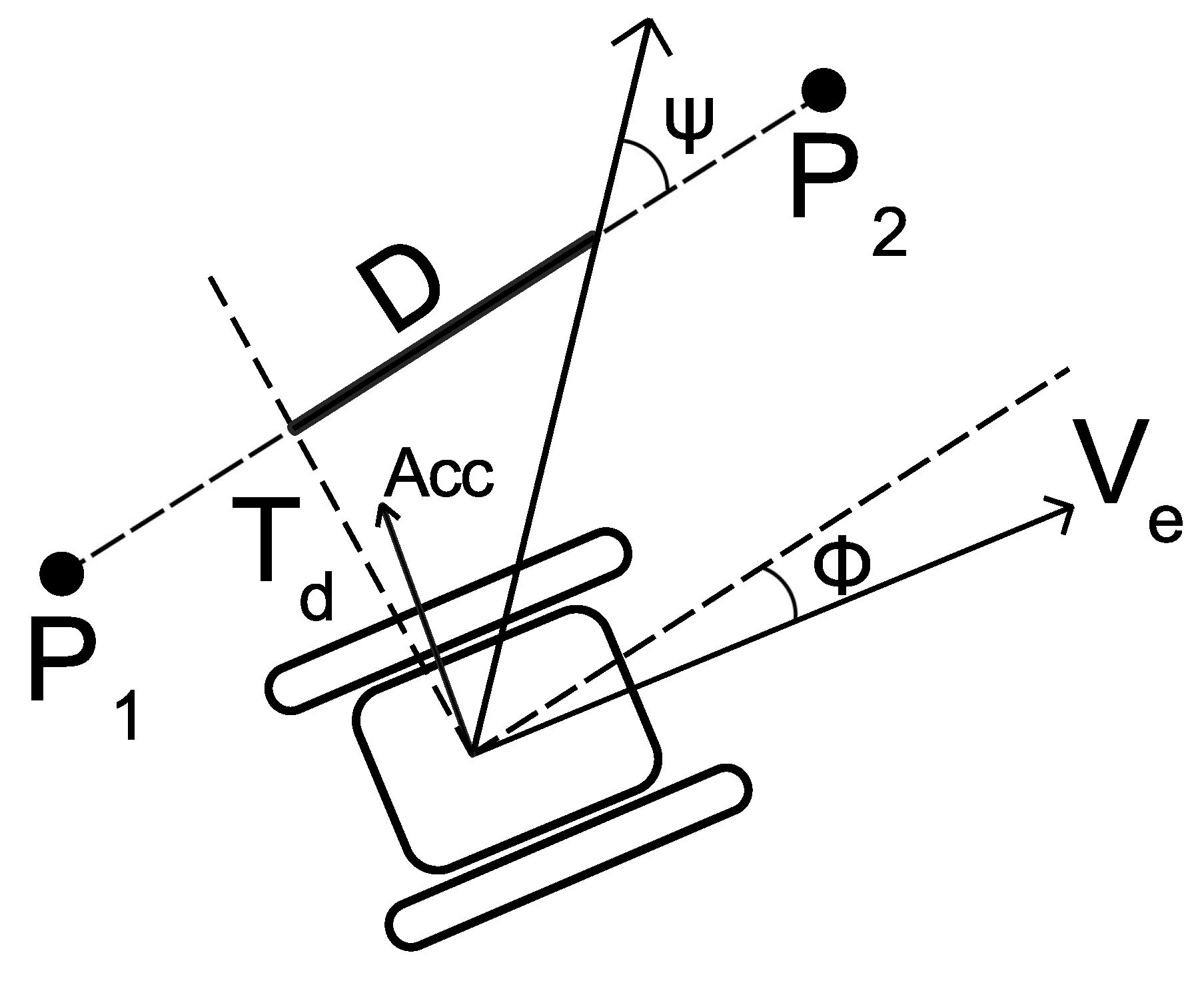
The path following strategy relies on a reference point that is placed on the desired trajectory and on the generation of a lateral acceleration based on the reference point, which is then converted into corresponding PWM commands of the drive motors thanks to the use of a PID controller. PWM values from 900 µs to 1450 µs cause the motors to spin counterclockwise, while values from 1550 µs to 1900 µs command the motor to spin clockwise. Figure 7 shows a typical trajectory, where P1 and P2 are the successive waypoints to follow, is the longitudinal velocity of the vehicle, is the along-track distance, which is defined as the horizontal distance between the vehicle’s current position and a reference point on the desired trajectory; D is the distance between and a generic point on the trajectory as a momentary goal, while and are the correction angles relative to the trajectory from towards . The lateral acceleration for the trajectory correction [43], which is a type of banking turn for the vehicle, can be described as:
where the parameter K is an integer value used to adjust the algorithm and avoid overshooting during the trajectory tracking.
The direction of the lateral acceleration depends on the position of the generic reference point on the path compared to the longitudinal velocity vector of the vehicle . For instance, if the reference point is to the left of the velocity vector and < 20, then the controller will generate the PWM signals to command the left motor (i.e., µs) to decrease its forward velocity, while increasing the velocity on the right motor (i.e., µs) in order to allow the vehicle to change its orientation, pointing towards the reference point. Furthermore, if > 20, then the vehicle is supposed to be too far from the reference point and therefore the controller changes the spinning direction of one motor (i.e., µs) as compared to the second motor (i.e., µs) to perform a turn-on-the-spot rotation. The PID parameters for the controller were empirically determined as , , and allow a smooth convergence to the desired path by minimizing the distance along the track . For more details, the interested reader is referred to [44]
4. Experimental Results
4.1. Path following Validation
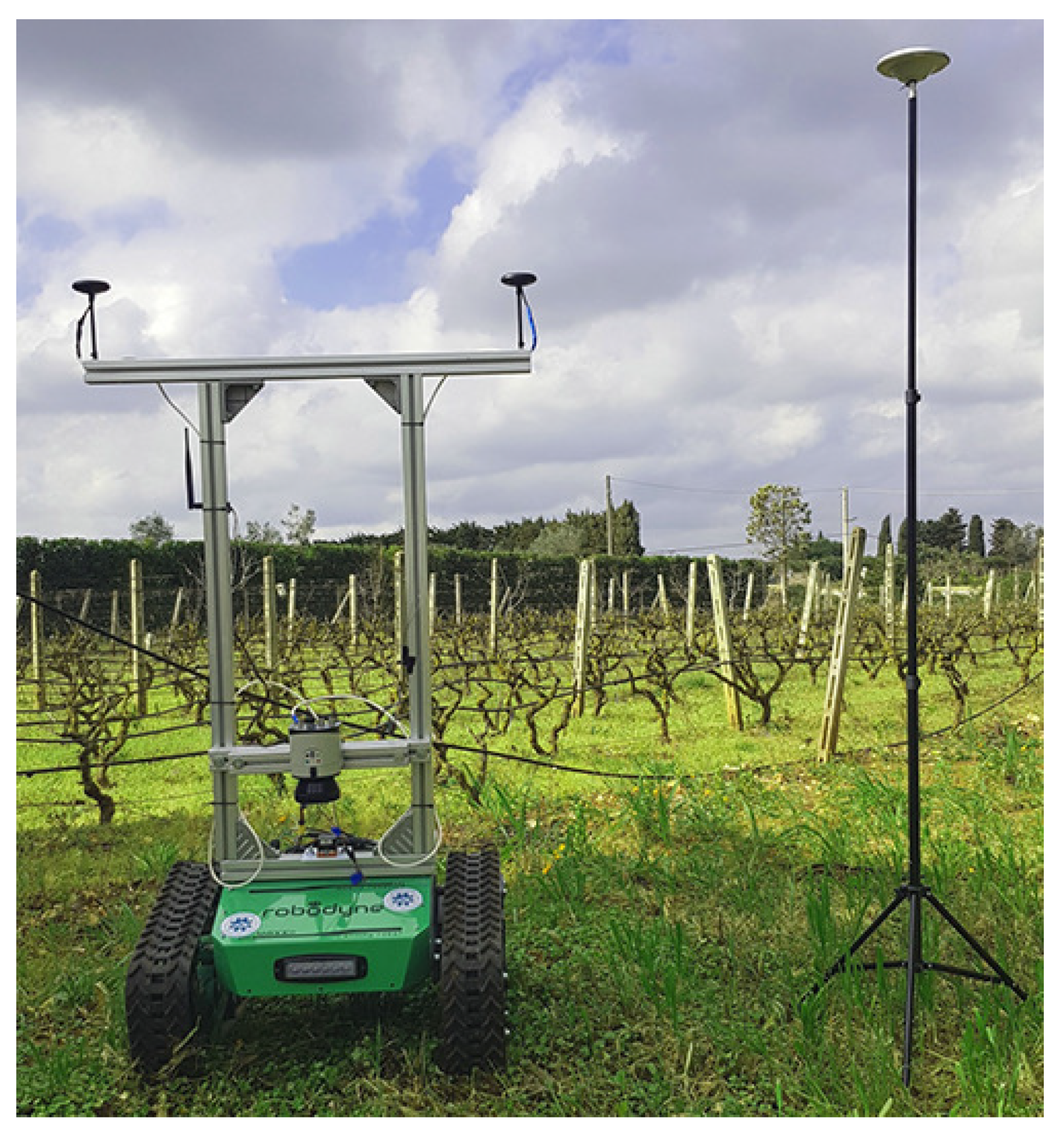
Several experimental tests have been performed on a farmland located in San Cassiano, South of Italy, in order to validate RoboNav. Before beginning the experiments, with a clear sky, the GPS base station was placed and installed in the field to run the static calibration procedure needed to achieve an accuracy of ±0.1 m for the RTK mode running at 10 Hz. Figure 8 shows the setup used for the tests.
Afterwards, a set of GPS waypoints was generated by using Google Earth in order to drive the vehicle along the vineyard, which includes a total of twelve rows. However, from the preliminary calibration stage, it was found that the GPS waypoints selected via Google Earth were affected by bias errors [45]. Therefore, a different strategy has been adopted in order to define the desired path: the vehicle has been driven along the the vineyard by a remote operator while collecting a certain number of waypoints as estimated by the GPS. Figure 9 shows the desired path loaded on a mission planner software program, as obtained by interpolation of the pre-learned collected waypoints. One of the most important aspects to consider is how the vehicle performs at the end of the row, where a very tight steering maneuver is required in a limited operating space with only a terrain patch of 1.5 × 1.5 m available. Then, the vehicle has been placed at the beginning of the first row and commanded to follow autonomously the pre-planned path ten times, by running each loop at different times of the day with different weather conditions, both with clear sky and cloudy, and by driving on different kinds of terrain surfaces, i.e., at the beginning of the row, the terrain is flat and compact, while in the middle, it is ploughed. Various tests have been also performed with the use of a single GPS receiver. Unfortunately, the heading provided by the single GPS sensor did not allow the vehicle to drive safely along the rows, leading to continuous stops due to obstacle detection warnings. A dedicated test for the direct comparison of the dual and single GPS configuration is presented later in Section 4.4.
Figure 10 highlights the discrepancy between the reference path, in black, and the path autonomously followed by the robot, in red, using RoboNav during test 8. It is worth noticing that the sampling rate used for collecting the data is 20 Hz for each test. To make all the graphs more readable, a 3-D coordinate transformation function has been applied to convert latitude, longitude coordinates to x,y coordinates in a local Cartesian coordinate system. It can be observed how the followed path almost overlaps the reference path during straight trajectories, while they deviate slightly during the turning maneuver and also for few meters after the steering, before returning to the correct track for the straight trajectory, as it is possible to observe in Figure 11. In this specific test, the deviation error from the reference path registered while driving along the first row is cm for the x axis, whereas the deviation error on the headland is cm, while the maximum deviation error is reported when the vehicle tries to enter the next row shortly after the steering maneuver with cm. For each test, the error deviation between the reference path and the followed path has been measured both for straight and steering maneuvers by using a tape measure and props to mark the position of the vehicle. Table 2 reports the errors , along the x,y axis and for the heading estimation measured for each loop and shows how the maximum error is always registered during the steering maneuver, while all the errors for the straight path have been measured immediately after the steering operation, and this is due to the fact that the control algorithm tries to reach the desired position by facing also the classic slipping effects caused by the different velocities applied on each track. The average error along the x axis is cm, while on the y axis, it is cm. The average error in the heading estimation is , showing how the use of two GPS modules with multiple EKF instances is able to provide a steady heading prediction. It is worth noticing that test 8 is affected by large errors since it has been performed with an overcast sky with a reduced number of satellites.
4.2. Performance with Limited Number of Visible Satellites
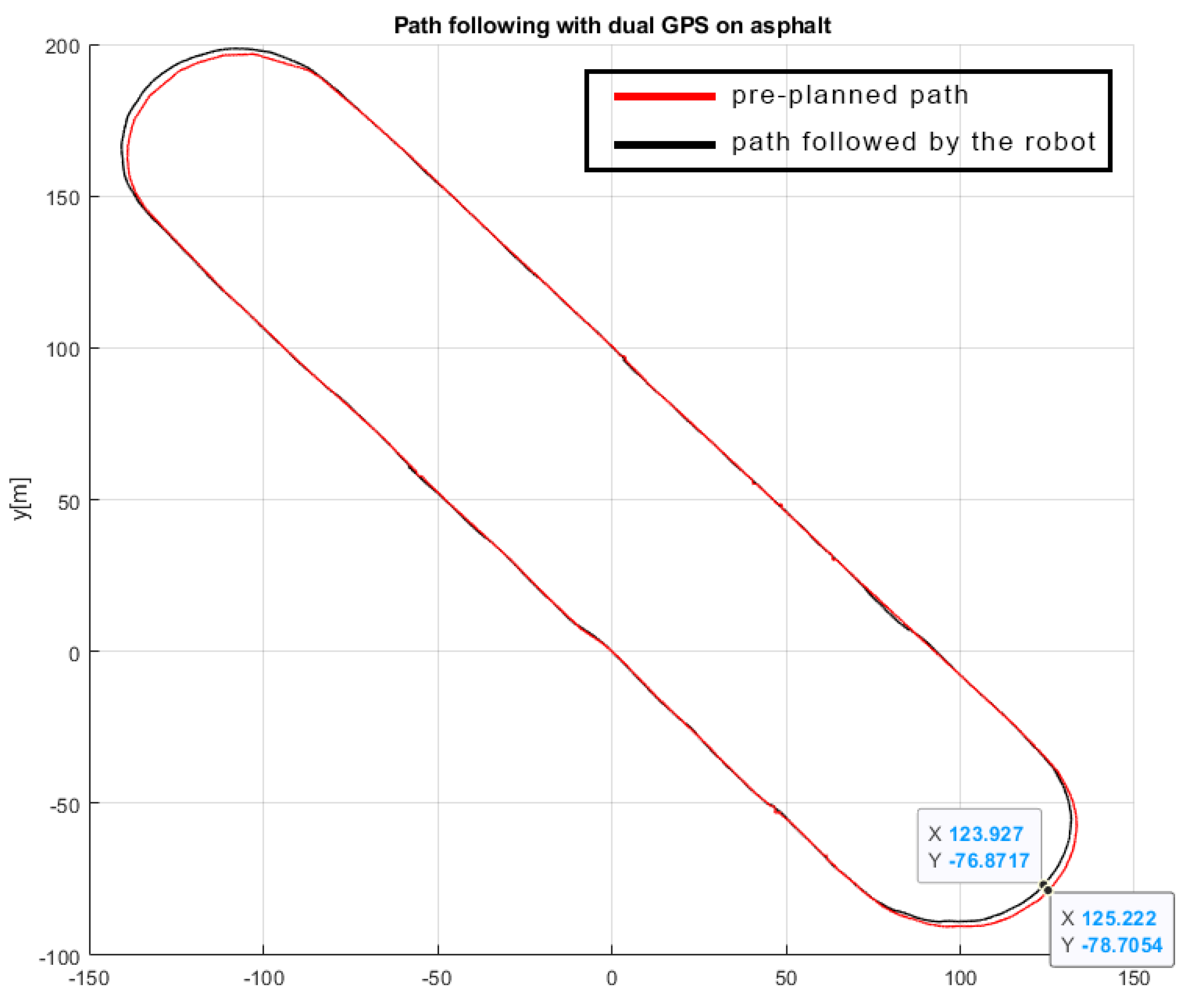
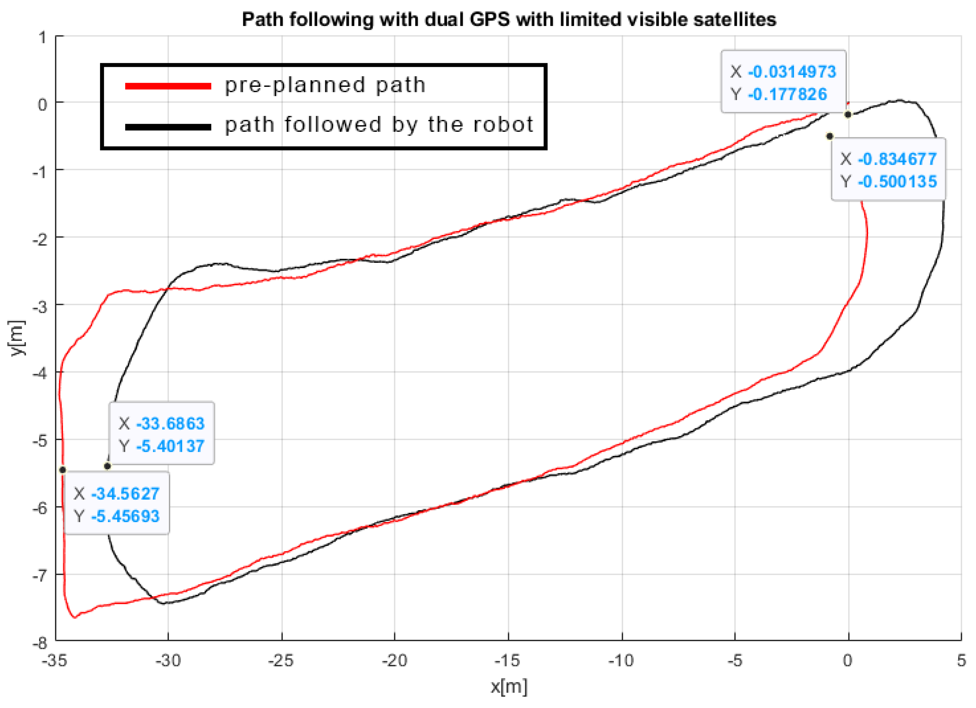
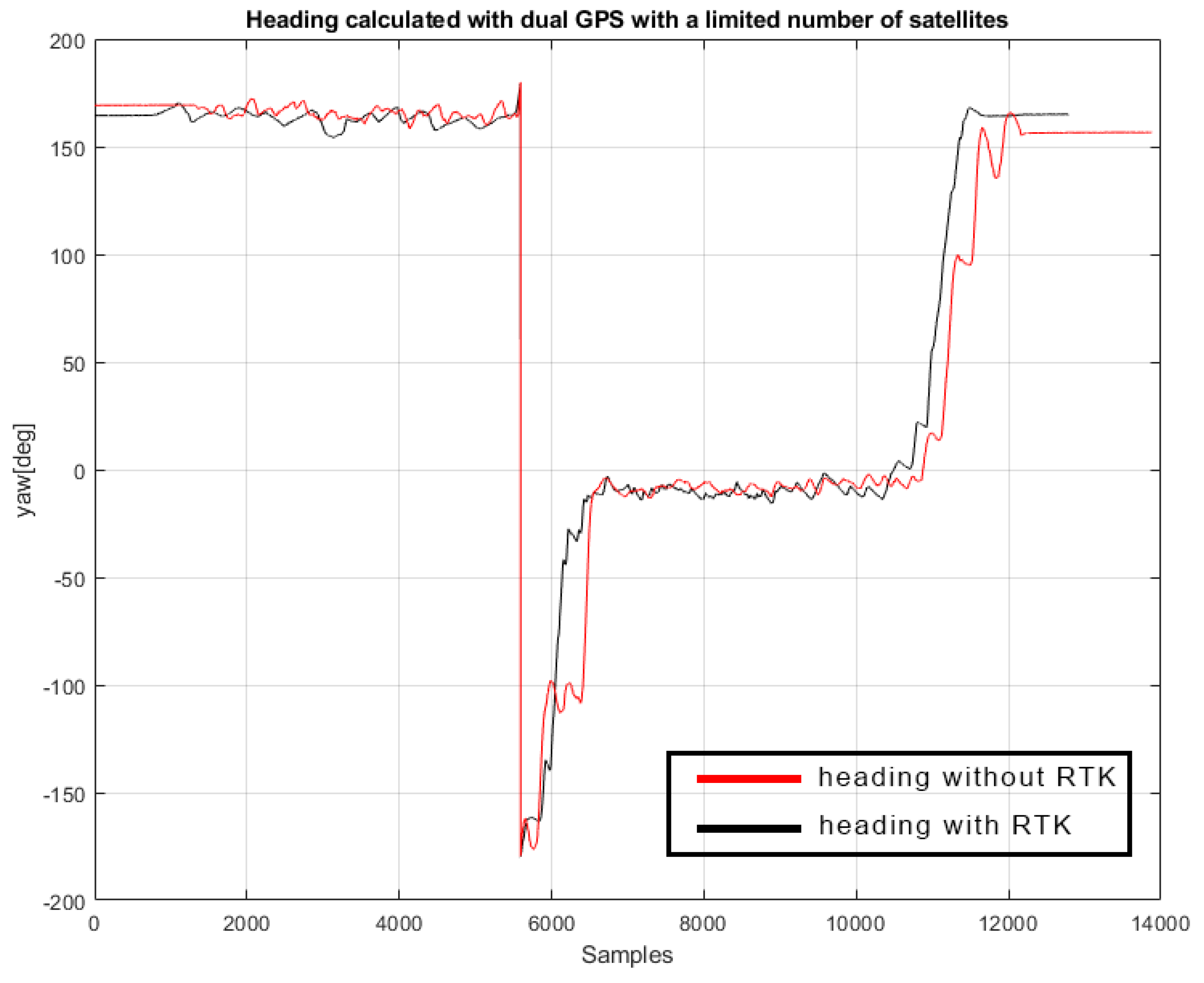
Additional tests have been carried out to evaluate the performance of the path following algorithm based on the number of satellites visible in the sky. Figure 12 highlights the performance of the tracking algorithm when the vehicle is commanded to autonomously follow a closed-loop path on an asphalt runway with a reduced number of visible satellites, with the GPS status ranging from single precision to RTK float mode. It is interesting to note how the straight trajectories perfectly overlap, while a maximum deviation error m is registered on the curved trajectory. Figure 13 shows the results of another test that has been carried out in a steep slope vineyard by commanding the vehicle to move down the first row and to climb to the starting position by moving along the next row. In this case, the maximum deviation error m registered when the vehicle switches between the rows is partly due to the reduced number of visible satellites but also to the efforts made by the tracking controller to keep the vehicle on its track, since it is forced to execute a steering maneuver while facing a slope of more than 10, as reported in Figure 14. It is relevant to observe that the navigation system is able to generate a consistent heading even when the RTK mode is not steady, by providing heading errors that range from 0.1 to 0.3, as highlighted in Figure 15, by relying on the position of the two GPS modules, as described in Section 2.1. One of the key aspects of the use of two GPS modules is that it is always possible to calculate the vehicle heading, even if the GPS receivers are not in RTK mode, as long as their positioning error is less than cm, which is the distance between GPS1 and GPS2, as reported in Figure 2.
4.3. Tracking Controller Evaluation
It is critical to be able to accurately estimate the vehicle yaw in order to increase the performance of the tracking controller. Figure 16 reports the performance for the yaw tracking by comparing the desired orientation, in black, versus the actual heading of the vehicle, in red, respectively; as can be seen, the vehicle drives forward along the first straight path pointing almost to the North; in fact, the registered yaw is around , while it points towards the South during the second straight motion after the steering, with a registered value of around . It is worth highlighting that the yaw tracking is consistent along all the loop. The correct orientation reported by the system has been double-checked with an external digital compass oriented according with the orientation of the vehicle—in particular, a TRAX2 AHRS digital compass able to provide superior heading and orientation under a wide range of demanding conditions has been used as ground truth to validate the performance of the system.
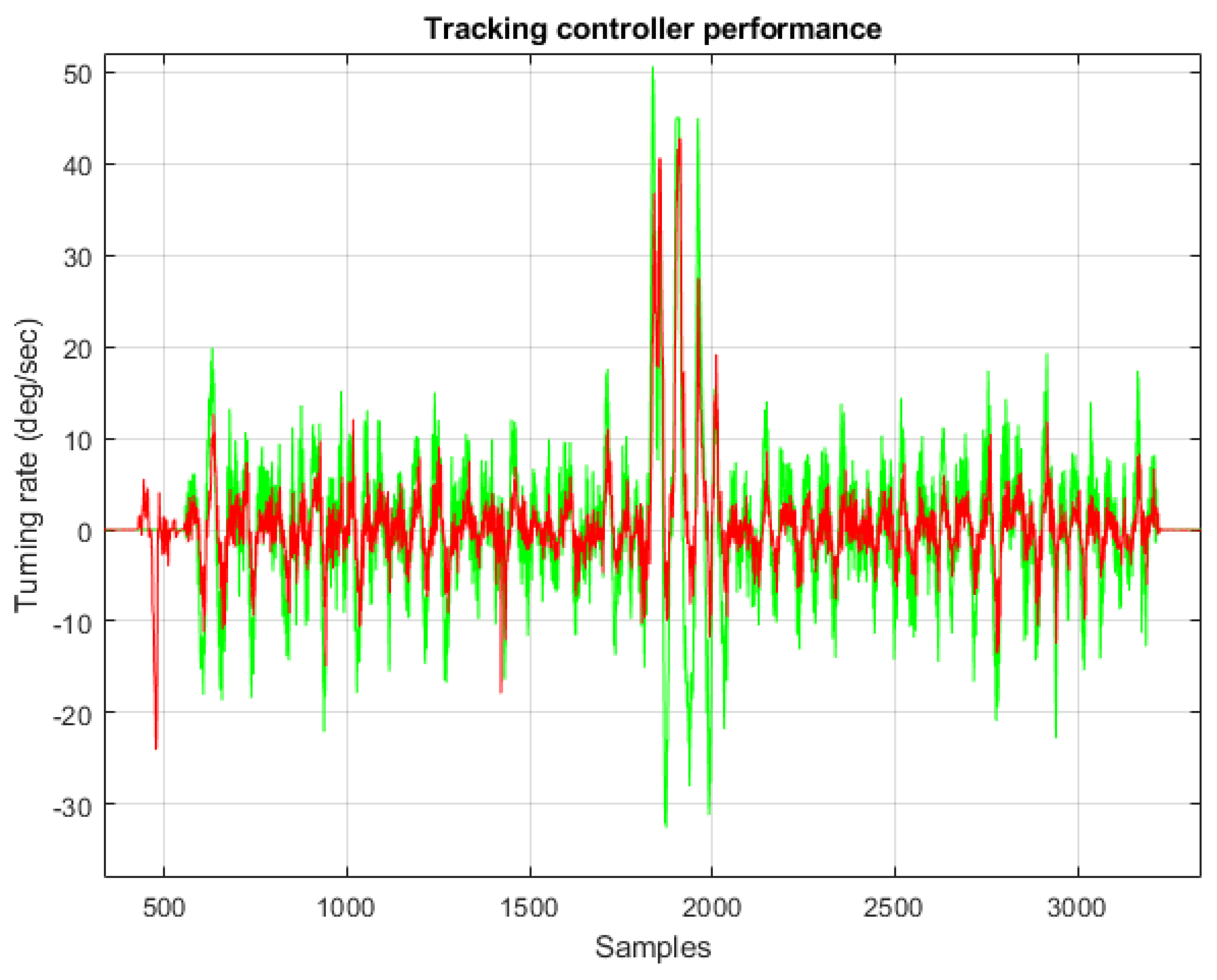
Figure 17 depicts the overall performance of the tracking controller, where the red line is the desired speed m/s set by the controller, the blue line is the integral controller correction trying to adjust the generated speed command, while the green line is the actual speed for the vehicle that ranges from 0.30 m/s to 0.32 m/s. It is important to note that all the tests were performed with a forward velocity of 0.3 m/s, which equals 50% of the maximum velocity of the vehicle (0.6 m/s). It is chosen as a conservative speed in consideration of the full autonomy of the navigation system. Higher velocities would have entailed higher risks for the robot and the environment. Nevertheless, this velocity is found to be a good trade-off between safety and efficiency, as the farmer robot is able to survey a vineyard of 1 hectare (50 rows of 100 m length) in around 25 min. Moreover, by looking at Figure 18, it should be noted that the generated output for the turning rate, which is the red line, is able to correctly follow the desired angular velocity marked by the green color; moreover, it is interesting to see how the controller produces small corrections even along the straights in order to follow the desired path and to minimize the along-track distance , as described in Section 3.1, whereas it introduces a desired turning rate of up to 40/s to face the turning maneuver.
The small corrections are also related to compensation effects strictly caused by slipping effects on soft agricultural terrain, as it is also possible to verify during the first 600 samples, where some spikes in the actual turning rate have been registered before the controller started the corrections. Finally, Figure 19 shows the motor controller output provided by the motor control board to command both the left and right motor in blue and red color, respectively. In this case, it is particularly interesting to note how only the left track is subjected to an increase in the turning speed, since the vehicle steers on the right when it reaches the end of the first row, while the right track only tries to compensate for the skidding effects since the maneuver is very tight.
4.4. Dual GPS vs. Single GPS Navigation
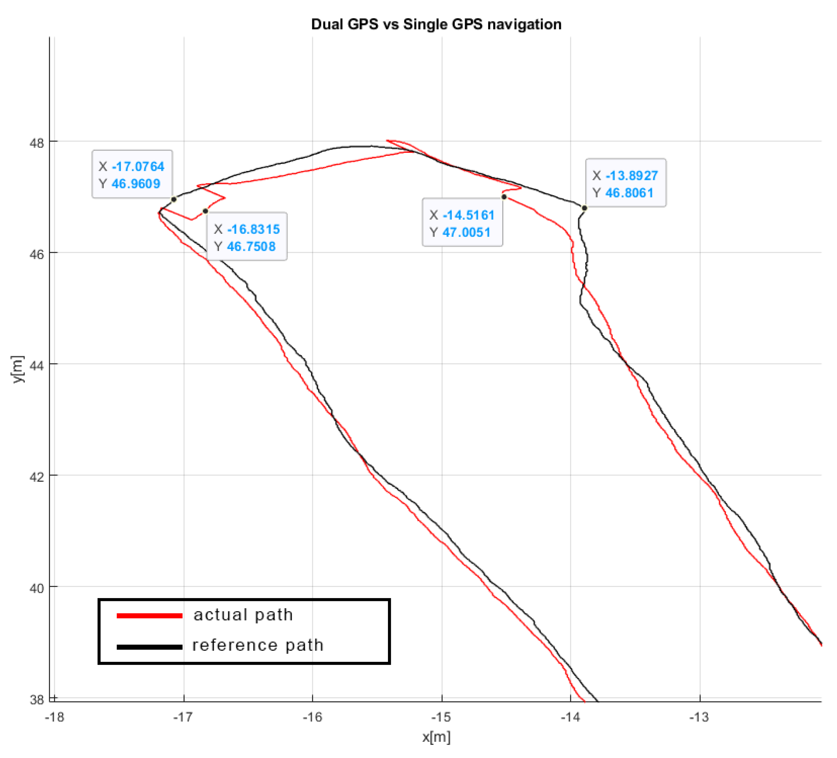
Various tests have been also performed with the use of a single GPS receiver placed in the center of the fixed baseline in order to compare the localization and the heading estimation capabilities without using two GPS receivers. The first test was performed by commanding the vehicle to follow the path previously generated to run the tests in Section 4.1 and described in Figure 9. Unfortunately, while the localization was still acceptable mostly for the straight trajectories, the heading provided by the single GPS sensor did not allow the vehicle to drive safely along the row, especially during the steering on the headland at the end of the first row, leading to continuous stops due to obstacle detection warnings. Figure 20 includes an enlarged view of the turning maneuver that highlights how the vehicle failed the heading estimation twice and was forced to stop to avoid collisions with the vine plants. The maximum error m registered in this test would have been greater with the vehicle free to move around the field. As shown in Figure 21, an additional test has been performed in a obstacle-free zone by commanding the vehicle to follow a closed loop with both the straight trajectories that overlap for a short section. As reported in Figure 22, following the black line, the vehicle begins to move pointing towards North-East, and then it turns almost on the spot and moves back to the starting position pointing to South-East. Even in this test, the system failed to correctly estimate the heading by losing the consistency of all the EKF instances and by forcing the vehicle to change its direction with an unpredictable behavior. These tests demonstrate how the heading estimation is reliable only when using the dual GPS configuration. For safety purposes, a routine has been included in the navigation software in order to stop the vehicle if the signal from both the GPS modules is lost.
5. Conclusions
A cost-effective and high-precision autonomous navigation system for agriculture applications has been presented, along with a series of experimental tests in real settings. A dual GPS configuration based on two u-blox modules in conjunction with three low-cost inertial sensors has been used to run a Gaussian Sum Filter capable of combining multiple Extended Kalman Filters. The system was able to provide estimation of both position and heading with high precision and robustness, by dealing with IMU bias and GPS signal loss, minimizing the crosstrack error and showing average errors on the order of 0.2 m and 0.2 for the measurement of position and yaw angle, respectively. The total cost of the proposed solution is around 1300 EUR, which is significantly lower when compared to commercial solutions based on professional dual-antenna GPS. The tracking controller used for the path following algorithm performed as expected, and the vehicle was correctly able to traverse one or more vineyard rows autonomously. In addition, the controller has also been tested in narrow spaces where tight steering operations are requested to allow the vehicle to adjust its position to move out of the previous row and enter the next one. Future work will rely on the integration of a 3D laser sensor and RGB-D cameras for mapping and obstacle avoidance, to improve the controller’s performance, particularly also when the GPS signal is weak or when only a GPS module can be used. Alternative control strategies for path tracking will be also investigated to further improve the system’s performance.
Author Contributions
All authors contributed equally to the writing of this manuscript. All authors have read and agreed to the published version of the manuscript.
Funding
The financial support of the projects Agricultural in TeroperabiLity and Analysis System (ATLAS), H2020 (Grant No. 857125), and multimodalsensing for individual plANT phenOtyping in agriculture robotics (ANTONIO), ICTAGRI-FOOD COFUND (Grant No. 41946) is gratefully acknowledged.
Institutional Review Board Statement
Not applicable.
Informed Consent Statement
Not applicable.
Data Availability Statement
Data supporting the findings of this study are available from the corresponding author on request.
Conflicts of Interest
The authors declare no conflict of interest.
Abbreviations
The following abbreviations are used in this manuscript:
| LiDAR | Light Detection and Ranging |
| IMU | Inertial Measurement Unit |
| RTK | Real-time kinematic positioning |
| GSF | Gaussian Sum Filter |
| GPS | Global Positioning System |
References
- Shamshiri, R.; Weltzien, C.; Hameed, I.; Yule, I.; Grift, T.; Balasundram, S.; Pitonakova, L.; Ahmad, D.; Chowdhary, G. Research and development in agricultural robotics: A perspective of digital farming. Int. J. Agric. Biol. Eng. 2018, 11, 1–14. [Google Scholar] [CrossRef]
- Galati, R.; Mantriota, G.; Reina, G. Mobile Robotics for Sustainable Development: Two Case Studies. In Proceedings of the International Workshop IFToMM for Sustainable Development Goals, Online, 25–26 November 2022; pp. 372–382. [Google Scholar]
- Galati, R.; Mantriota, G.; Reina, G. Design and Development of a Tracked Robot to Increase Bulk Density of Flax Fibers. J. Mech. Robot. 2021, 13, 050903. [Google Scholar] [CrossRef]
- Raja, V.; Bhaskaran, B.; Nagaraj, K.; Sampathkumar, J.; Senthilkumar, S. Agricultural harvesting using integrated robot system. Indones. J. Electr. Eng. Comput. Sci. 2022, 25, 152. [Google Scholar] [CrossRef]
- Halstead, M.; McCool, C.; Denman, S.; Perez, T.; Fookes, C. Fruit Quantity and Ripeness Estimation Using a Robotic Vision System. IEEE Robot. Autom. Lett. 2018, 3, 2995–3002. [Google Scholar] [CrossRef]
- Galati, R.; Reina, G.; Messina, A.; Gentile, A. Survey and navigation in agricultural environments using robotic technologies. In Proceedings of the 2017 14th IEEE International Conference on Advanced Video and Signal Based Surveillance (AVSS), Lecce, Italy, 29 August–1 September 2017; pp. 1–6. [Google Scholar] [CrossRef]
- Vougioukas, S. Agricultural Robotics. Annu. Rev. Control. Robot. Auton. Syst. 2019, 2, 365–392. [Google Scholar] [CrossRef]
- Oliveira, L.F.; Silva, M.; Moreira, A. Agricultural Robotics: A State of the Art Survey. In Proceedings of the 23rd International Conference Series on Climbing and Walking Robots and the Support Technologies for Mobile Machines, Moscow, Russia, 24–26 August 2020; pp. 279–286. [Google Scholar] [CrossRef]
- Rahman, M.M.; Ishii, K. Heading Estimation of Robot Combine Harvesters during Turning Maneuveres. Sensors 2018, 18, 1390. [Google Scholar] [CrossRef]
- Zhang, Y.; Li, Y.; Huang, Y.; Liu, X.; Liu, C. A Path Tracking Method for Autonomous Rice Drill Seeder in Paddy Fields. In Proceedings of the 2018 2nd International Conference on Mechanical, System and Control Engineering (ICMSC 2018), Moscow, Russia, 21–23 June 2018; Volume 220, p. 04004. [Google Scholar] [CrossRef]
- Yin, X.; Wang, Y.; Chen, Y.; Jin, C.; Du, J. Development of autonomous navigation controller for agricultural vehicles. Int. J. Agric. Biol. Eng. 2020, 13, 70–76. [Google Scholar] [CrossRef]
- Taka, R.; Barawid, O.; Ish, K.; Noguch, N. Development of Crawler-Type Robot Tractor based on GPS and IMU. IFAC Proc. Vol. 2010, 43, 151–156. [Google Scholar] [CrossRef]
- Ojeda, L.; Reina, G.; Cruz, D.; Borenstein, J. The FLEXnav precision dead-reckoning system. Int. J. Veh. Auton. Syst. 2006, 4, 173–195. [Google Scholar] [CrossRef]
- Yu, S.; Jiang, Z. Design of the navigation system through the fusion of IMU and wheeled encoders. Comput. Commun. 2020, 160, 730–737. [Google Scholar] [CrossRef]
- Guevara, D.J.; Gené-Mola, J.; Gregorio, E.; Torres-Torriti, M.; Reina, G.; Cheein, F.A.A. Comparison of 3D scan matching techniques for autonomous robot navigation in urban and agricultural environments. J. Appl. Remote Sens. 2021, 15, 173–195. [Google Scholar] [CrossRef]
- Malavazi, F.; Guyonneau, R.; Fasquel, J.B.; Lagrange, S.; Mercier, F. LiDAR-only based navigation algorithm for an autonomous agricultural robot. Comput. Electron. Agric. 2018, 154, 71–79. [Google Scholar] [CrossRef]
- Alatise, M.; Hancke, G. Pose Estimation of a Mobile Robot Based on Fusion of IMU Data and Vision Data Using an Extended Kalman Filter. Sensors 2017, 17, 2164. [Google Scholar] [CrossRef] [PubMed]
- Tsun, M.T.K.; Lau, B.T.; Jo, H.S. Exploring the Performance of a Sensor-Fusion-based Navigation System for Human Following Companion Robots. Int. J. Mech. Eng. Robot. Res. 2018, 7, 590–598. [Google Scholar] [CrossRef]
- Ma, D.M.; Shiau, J.K.; Wang, I.C.; Lin, Y.H. Attitude Determination Using a MEMS-Based Flight Information Measurement Unit. Sensors 2012, 12, 1–23. [Google Scholar] [CrossRef]
- Abbas, M.; Kamel, A.; Elhalwagy, Y.; Albordany, R. Performance Enhancement of Low Cost Non-GPS Aided INS for Unmanned Applications. In Proceedings of the International Conference on Aerospace Sciences and Aviation Technology, Cairo, Egypt, 28–30 May 2013; Volume 15, pp. 1–18. [Google Scholar] [CrossRef]
- Mihajlow, R.; Demirev, V. Application of GPS navigation in agricultural aggregates. Annu. J. Tech. Univ. Varna Bulg. 2018, 2, 14–19. [Google Scholar] [CrossRef] [Green Version]
- Lan, H.; Elsheikh, M.; Abdelfatah, W.; Wahdan, A.; El-Sheimy, N. Integrated RTK/INS Navigation for Precision Agriculture. In Proceedings of the 32nd International Technical Meeting of the Satellite Division of the Institute of Navigation, Miami, FL, USA, 16–20 September 2019; pp. 4076–4086. [Google Scholar] [CrossRef]
- Kaartinen, H.; Hyyppa, H. Accuracy of Kinematic Positioning Using Global Satellite Navigation Systems under Forest Canopies. Forests 2015, 6, 3218–3236. [Google Scholar] [CrossRef]
- Yudanto, R.; Ompusunggu, A.P.; Bey-Temsamani, A. On improving low-cost IMU performance for online trajectory estimation. In Proceedings of the Smart Sensors, Actuators, and MEMS VII; and Cyber Physical Systems, Barcelona, Spain, 4–6 May 2015; Volume 9517, pp. 639–650. [Google Scholar] [CrossRef]
- Eun-Hwan, S.; El-Sheimy, N. Accuracy Improvement of Low Cost INS/GPS for Land Applications. In Proceedings of the 2002 National Technical Meeting of The Institute of Navigation, San Diego, CA, USA, 28–30 January 2001. [Google Scholar]
- Consoli, A.; Ayadi, J.; Bianchi, G.; Pluchino, S.; Piazza, F.; Baddour, R.; Parés, M.E.; Navarro, J.; Colomina, I.; Gameiro, A.; et al. A multi-antenna approach for UAV’s attitude determination. In Proceedings of the 2015 IEEE Metrology for Aerospace (MetroAeroSpace), Benevento, Italy, 4–5 June 2015; pp. 401–405. [Google Scholar] [CrossRef]
- Nadarajah, N.; Teunissen, P.J.G.; Raziq, N. Instantaneous GPS–Galileo Attitude Determination: Single-Frequency Performance in Satellite-Deprived Environments. IEEE Trans. Veh. Technol. 2013, 62, 2963–2976. [Google Scholar] [CrossRef]
- Henkel, P.; Günther, C. Attitude determination with low-cost GPS/INS. In Proceedings of the 26th International Technical Meeting of the Satellite Division of the Institute of Navigation, ION GNSS 2013, Nashville, TN, USA, 16–20 September 2013; Volume 3, pp. 2015–2023. [Google Scholar]
- Eling, C.; Klingbeil, L.; Kuhlmann, H. Real-time single-frequency GPS/MEMS-IMU attitude determination of lightweight UAVs. Sensors 2015, 15, 26212–26235. [Google Scholar] [CrossRef]
- Tu, X.; Tang, L. Headland Turning Optimisation for Agricultural Vehicles and Those with Towed Implements. J. Agric. Food Res. 2019, 1, 100009. [Google Scholar] [CrossRef]
- Peng, C.; Fei, Z.; Vougioukas, S. Depth camera based row-end detection and headland maneuvering in orchard navigation without GNSS. In Proceedings of the 30th Mediterranean Conference on Control and Automation, Athens, Greece, 28 June–1 July 2022. [Google Scholar]
- Loukatos, D.; Petrongonas, E.; Manes, K.; Kyrtopoulos, I.V.; Dimou, V.; Arvanitis, K.G. A Synergy of Innovative Technologies towards Implementing an Autonomous DIY Electric Vehicle for Harvester-Assisting Purposes. Machines 2021, 9, 82. [Google Scholar] [CrossRef]
- Winterhalter, W.; Fleckenstein, F.; Dornhege, C.; Burgard, W. Localization for precision navigation in agricultural fields—Beyond crop row following. J. Field Robot. 2021, 38, 429–451. [Google Scholar] [CrossRef]
- Shah, H.; Mehta, K.; Gandhi, S. Autonomous Navigation of 3 Wheel Robots Using Rotary Encoders and Gyroscope. In Proceedings of the 2014 International Conference on Computational Intelligence and Communication Networks, Bhopal, MP, USA, 14–16 November 2014; pp. 1168–1172. [Google Scholar] [CrossRef]
- Alsalamy, S.; Foo, B.; Frels, G. Autonomous Navigation and Mapping Using LiDAR. 2018. Available online: https://digitalcommons.calpoly.edu/cgi/viewcontent.cgi?article=1302&context=cpesp (accessed on 1 April 2022).
- Fan, Z.; Li, Z.; Cui, X.; Lu, J. Precise and Robust RTK-GNSS Positioning in Urban Environments with Dual-Antenna Configuration. Sensors 2019, 19, 3586. [Google Scholar] [CrossRef] [PubMed]
- Zhang, J. Autonomous navigation for an unmanned mobile robot in urban areas. In Proceedings of the 2011 IEEE International Conference on Mechatronics and Automation, Beijing, China, 7–10 August 2011; pp. 2243–2248. [Google Scholar] [CrossRef]
- Cepe, A. True Heading Estimation Using Two Gps Receivers And Carrier Phase Observables. In Proceedings of the 9th Saint Petersburg International Conference on Integrated Navigation Systems, St. Petersburg, Russia, 26–28 May 2012. [Google Scholar]
- Azdy, R.; Darnis, F. Use of Haversine Formula in Finding Distance Between Temporary Shelter and Waste End Processing Sites. J. Phys. Conf. Ser. 2020, 1500, 012104. [Google Scholar] [CrossRef]
- Meier, L.; Honegger, D.; Pollefeys, M. PX4: A node-based multithreaded open source robotics framework for deeply embedded platforms. In Proceedings of the IEEE International Conference on Robotics and Automation, Seattle, WA, USA, 26–30 May 2015; Volume 2015, pp. 6235–6240. [Google Scholar] [CrossRef]
- Github. C++ Navigation Libraries. 2021. Available online: https://github.com/ArduPilot/ardupilot/tree/master/Rover (accessed on 1 April 2022).
- Savage, P.G. Strapdown Inertial Navigation Integration Algorithm Design Part 2: Velocity and Position Algorithms. J. Guid. Control. Dyn. 1998, 21, 208–221. [Google Scholar] [CrossRef]
- Fernandes, M.; Vinha, S.; Paiva, L.; Fontes, F. L0 and L1 Guidance and Path-Following Control for Airborne Wind Energy Systems. Energies 2022, 15, 1390. [Google Scholar] [CrossRef]
- Park, S.; Deyst, J.; How, J. A New Nonlinear Guidance Logic for Trajectory Tracking. In Proceedings of the AIAA Guidance, Navigation, and Control Conference and Exhibit, Monterey, CA, USA, 5–8 August 2004. [Google Scholar] [CrossRef] [Green Version]
- Zomrawi, N.; Mohammed, H. Positional Accuracy Testing of Google Earth. Int. J. Multidiscip. Sci. Eng. 2013, 4, 2045–7057. [Google Scholar]
Figure 1.
The wiring harness for the F9P GPS modules.

Figure 2.
Heading estimation, where p1 and p2 are the coordinates reported by each GPS module in RTK mode; P is the vehicle position located on the baseline b = 100 cm. The GPS antennas coincide with the GPS module position.
Figure 2.
Heading estimation, where p1 and p2 are the coordinates reported by each GPS module in RTK mode; P is the vehicle position located on the baseline b = 100 cm. The GPS antennas coincide with the GPS module position.

Figure 3.
A sample wiring harness for the three IMU modules showing the main components used for the connections. Note that a 10 pF capacitor was also used on the I2C bus (not shown in figure).
Figure 3.
A sample wiring harness for the three IMU modules showing the main components used for the connections. Note that a 10 pF capacitor was also used on the I2C bus (not shown in figure).

Figure 4.
The rubber tracked vehicle during the experimental tests.

Figure 5.
The overall hardware architecture used for this research study.

Figure 6.
The block diagram for yaw angle estimation based on the three EKF instances and the attitude and heading reference system (AHRS) obtained as a combination between GPS and the three inertial sensors.
Figure 6.
The block diagram for yaw angle estimation based on the three EKF instances and the attitude and heading reference system (AHRS) obtained as a combination between GPS and the three inertial sensors.

Figure 7.
A typical configuration of the robot moving from P1 to P2.

Figure 8.
On the left, the vehicle with the dual GPS system. On the right, the base station antenna.
Figure 8.
On the left, the vehicle with the dual GPS system. On the right, the base station antenna.

Figure 9.
A typical pre-planned path in a vineyard. Green label: waypoints. Yellow line: interpolated path.
Figure 9.
A typical pre-planned path in a vineyard. Green label: waypoints. Yellow line: interpolated path.

Figure 10.
A comparison between the pre-planned path made by remotely controlling the vehicle, in black, and the path followed by the robot driving autonomously using RoboNav, in red.
Figure 10.
A comparison between the pre-planned path made by remotely controlling the vehicle, in black, and the path followed by the robot driving autonomously using RoboNav, in red.

Figure 11.
Details related to the headland turning agility at the end of the first vineyard row, where the maximum displacement error is registered at the end of the steering maneuver.
Figure 11.
Details related to the headland turning agility at the end of the first vineyard row, where the maximum displacement error is registered at the end of the steering maneuver.

Figure 12.
A comparison between a closed-loop path on asphalt made by remotely controlling the vehicle used as a reference, in black, and the path followed by the vehicle, in red, with a reduced number of visible satellites.
Figure 12.
A comparison between a closed-loop path on asphalt made by remotely controlling the vehicle used as a reference, in black, and the path followed by the vehicle, in red, with a reduced number of visible satellites.

Figure 13.
The reference path, in black, and the followed path, in red, for a steep slope vineyard with a reduced number of visible satellites.
Figure 13.
The reference path, in black, and the followed path, in red, for a steep slope vineyard with a reduced number of visible satellites.

Figure 14.
The variation in slope in the vineyard used for the test.

Figure 15.
Heading calculated with the dual GPS system while operating with a limited number of visible satellites.
Figure 15.
Heading calculated with the dual GPS system while operating with a limited number of visible satellites.

Figure 16.
Desired yaw vs. actual yaw using the dual GPS configuration during test 8.

Figure 17.
Performance for the tracking controller during test 8: the red line is the desired speed, the blue line is the integral controller, while the green line is the actual speed of the vehicle.
Figure 17.
Performance for the tracking controller during test 8: the red line is the desired speed, the blue line is the integral controller, while the green line is the actual speed of the vehicle.

Figure 18.
Turning rate and desired turning rate for test 4: the green line is the desired angular velocity, while the red line is the generated turning rate.
Figure 18.
Turning rate and desired turning rate for test 4: the green line is the desired angular velocity, while the red line is the generated turning rate.

Figure 19.
PWM output generated for motor control: the red line is for the left motor while the right one is for the right motor.
Figure 19.
PWM output generated for motor control: the red line is for the left motor while the right one is for the right motor.

Figure 20.
Navigation test using dual and single GPS configurations in a vineyard, in black and red lines, respectively; the vehicle was stopped multiple times in single GPS mode due to obstacle detection warnings.
Figure 20.
Navigation test using dual and single GPS configurations in a vineyard, in black and red lines, respectively; the vehicle was stopped multiple times in single GPS mode due to obstacle detection warnings.

Figure 21.
Navigation test using dual and single GPS configuration: the test was stopped due to safety issues since the vehicle ran off the track.
Figure 21.
Navigation test using dual and single GPS configuration: the test was stopped due to safety issues since the vehicle ran off the track.

Figure 22.
Heading estimation obtained from the dual GPS configuration, in black, and from the single GPS, in red.
Figure 22.
Heading estimation obtained from the dual GPS configuration, in black, and from the single GPS, in red.


Table 1.
List of the main components for the proposed navigation system.
| Part | Qty | Type | Cost (€) | Total (€) |
|---|---|---|---|---|
| ZED-F9P | 3 | GPS | 180 | 540 |
| ICM | 3 | IMU | 30 | 90 |
| STM32 | 1 | CPU | 30 | 30 |
| RF | 3 | ANT | 12 | 36 |
| Total cost for the system | 696 | |||
Table 2.
Maximum errors reported over the ten tests to validate the path tracking control.
| Test | (cm) | (cm) | (°) |
|---|---|---|---|
| 1 | 12.20 | 15.20 | 0.10 |
| 2 | 12.50 | 15.10 | 0.12 |
| 3 | 12.40 | 14.40 | 0.20 |
| 4 | 13.10 | 14.00 | 0.12 |
| 5 | 12.90 | 14.00 | 0.17 |
| 6 | 13.8 | 13.90 | 0.11 |
| 7 | 12.00 | 13.50 | 0.20 |
| 8 | 18.85 | 19.43 | 0.20 |
| 9 | 13.5 | 15.00 | 0.17 |
| 10 | 12.90 | 15.60 | 0.12 |
Publisher’s Note: MDPI stays neutral with regard to jurisdictional claims in published maps and institutional affiliations. |
© 2022 by the authors. Licensee MDPI, Basel, Switzerland. This article is an open access article distributed under the terms and conditions of the Creative Commons Attribution (CC BY) license (https://creativecommons.org/licenses/by/4.0/).
Share and Cite
MDPI and ACS Style
Galati, R.; Mantriota, G.; Reina, G. RoboNav: An Affordable Yet Highly Accurate Navigation System for Autonomous Agricultural Robots. Robotics 2022, 11, 99. https://doi.org/10.3390/robotics11050099
AMA Style
Galati R, Mantriota G, Reina G. RoboNav: An Affordable Yet Highly Accurate Navigation System for Autonomous Agricultural Robots. Robotics. 2022; 11(5):99. https://doi.org/10.3390/robotics11050099
Chicago/Turabian StyleGalati, Rocco, Giacomo Mantriota, and Giulio Reina. 2022. "RoboNav: An Affordable Yet Highly Accurate Navigation System for Autonomous Agricultural Robots" Robotics 11, no. 5: 99. https://doi.org/10.3390/robotics11050099
Note that from the first issue of 2016, this journal uses article numbers instead of page numbers. See further details here.