
Effect of Stop-Loss Reinsurance on Primary Insurer Solvency


1
Department of Mathematical Sciences, University of Liverpool, Liverpool L69 3BX, UK
2
School for Business and Society, University of York, York YO10 5ZF, UK
3
Department of Mathematical Finance and Actuarial Science, Nankai University, Tianjin 300071, China
4
School of Mathematics, University of Edinburgh, Edinburgh EH9 3FD, UK
5
Stable, London EH8 9AB, UK
*
Author to whom correspondence should be addressed.
Risks 2022, 10(10), 193; https://doi.org/10.3390/risks10100193
Submission received: 7 September 2022
/
Revised: 29 September 2022
/
Accepted: 30 September 2022
/
Published: 10 October 2022
Abstract
:Stop-loss reinsurance is a risk management tool that allows an insurance company to transfer part of their risk to a reinsurance company. Ruin probabilities allow us to measure the effect of stop-loss reinsurance on the solvency of the primary insurer. They further permit the calculation of the economic capital, or the required initial capital to hold, corresponding to the 99.5% value-at-risk of its surplus. Specifically, we show that under a stop-loss contract, the ruin probability for the primary insurer, for both a finite- and infinite-time horizon, can be obtained from the finite-time ruin probability when no reinsurance is bought. We develop a finite-difference method for solving the (partial integro-differential) equation satisfied by the finite-time ruin probability with no reinsurance, leading to numerical approximations of the ruin probabilities under a stop-loss reinsurance contract. Using the method developed here, we discuss the interplay between ruin probability, reinsurance retention level and initial capital.
1. Introduction
The environment in which general insurance companies currently operate is challenging in at least two aspects. First, investment income is squeezed by unprecedented low levels of interest rates. Second, for some classes of businesses, premium rates are relatively low due to an abundance of industry capacity. Risk management is therefore relied upon not only for monitoring risks but also to inform management decisions.
A risk management tool often used by insurance companies is reinsurance, especially for very large risks or risks which are difficult to assess, for instance hurricanes, earthquakes or wildfires. Under a reinsurance contract, the reinsurer company agrees to compensate the primary insurer (or ceding company) for part of its insurance losses in exchange for a reinsurance premium. In short, reinsurance is when an insurance company transfers part of its underwritten insurance risks to a reinsurance company. By entering a reinsurance contract, the primary insurer should attain a reduction in the probability of incurring large losses and reduce the capital required to keep its insolvency risk at an acceptable level. There are different forms of reinsurance treaties, and for a review of their properties, we refer the reader to Albrecher et al. (2017). The choice of reinsurance treaty is complex, often relying on some optimality criteria related to profit, solvency and cost of capital (see, e.g., Haas 2012; Kull 2009) and taking into account the availability and price of the contract, market competition and regulatory constraints: see Albrecher et al. (2017) and references therein.
One form of reinsurance is stop-loss, under which the aggregate loss, over a given time period, is capped at an agreed retention level and the reinsurer is liable for the excess. This type of contract has been found to be optimal under different decision criteria, for instance, if the primary insurer wants to minimize the variance of the retained risk as per Borch, Kahn and Pesonen (e.g., see Pesonen 1984) or when maximizing expected utility in the context of risk-averse utility functions as per Arrow (1963) or Borch (1975). One can also model the solvency of a reinsurance strategy using the concept of ruin probability. Considering a ruin condition as the decision criterion allows to find the optimal reinsurance treaty for the insurer. Indeed, a stop-loss type of reinsurance contract is optimal when the criterion is to minimize the ruin probability: see Gajek and Zagrodny (2004). Minimizing the ruin probability and maximizing the expected utility are in fact related, as shown by Guerra and de Lourdes Centeno (2008, 2010) who again find that a stop-loss type of reinsurance contract is optimal under certain conditions.
Because it is based on the aggregate losses, compared with other types of reinsurance contracts, stop-loss is useful when it is difficult to allocate individual claims to particular events due to their nature, as can happen, for instance, in agriculture. From the risk management point of view, this type of treaty is special in the sense that it completely relieves the primary insurer from tail risk, a major concern for solvency. In this article, we introduce a methodology that allows us to study how stop-loss reinsurance affects the level of capital a primary insurer must hold to sustain a low level of insolvency risk determined by a strategic decision or regulatory directive. The regulatory solvency approach, under Solvency II, focusses on the one-year 99.5% value-at-risk, meaning that the probability that the aggregate loss over the year is larger than the available capital is 0.5%. Hence we use the 0.5% ruin probability to determine the level of economic capital necessary to cover the losses over the next year.
We first introduce a relationship between the finite and infinite-time ruin probability for a portfolio with stop-loss reinsurance, and the finite-time ruin probability for a portfolio with no reinsurance. Then, using a classical risk theory result, namely that the finite-time probability of ruin in a classical no-reinsurance contract satisfies an integro-partial differential equation (see Pervozvansky 1998), we proceed to numerically solve the equation and thus derive the finite-time-no-reinsurance ruin probability that leads to the finite and infinite-time ruin probability with stop-loss reinsurance.
We can then evaluate the level of risk faced by the primary insurer when covered by a stop-loss contract compared with the risk faced without taking on reinsurance. The risk cover provided by the reinsurance contract depends on the length of the contract. Remarkably, the stop-loss contract provides an upper bound to the ruin probability for a sufficiently long contract. In our numerical example, for a given set of parameters of the risk process, ruin probability plateaus for contracts longer than four months, showing that a realistic length of contract already provides such cap on the insolvency risk faced by the primary insurer. This shows the relevance of our results under realistic assumptions within a dynamic framework where the stop-loss contract can be regularly redefined in a finite (and not excessively large) time horizon.
As in any financial enterprise, the solvency of an insurer depends on its initial capital. Hence, it is important to understand the role of the initial capital on the solvency of the primary insurer and how it interacts with the amount of business ceded via a stop-loss contract. To that end, we evaluate the change in ruin probability, corresponding to different amounts of initial capital and different reinsurance retention levels. On the one hand, we conclude that ruin probability, and hence the risk of insolvency, is far more sensitive to the retention level for lower than higher levels of initial capital. On the other hand, decreasing the stop-loss retention level (or increasing the amount of risk ceded) does not imply a linear decrease in the initial capital required to maintain a chosen level of insolvency risk. At higher retention levels, the extra amount of initial capital necessary to compensate for retaining extra risk is lower than at lower retention levels. This implies that the motivation for the primary insurer to cede more risk to the reinsurer as a way of lowering the need of capital, and associated cost, reduces as the retention level increases. This is a convenient result in the sense that the primary insurer has diminishing incentive to seek an unlimited stop-loss contract. In fact, unlimited stop-loss contracts are not sold systematically (except under certain obligatory arrangements or captive solutions) because once the aggregate claim losses exceeds the agreed retention level the contract is a catastrophe for the reinsurer. In a dynamic finite-time horizon setting, a possible solution is for reinsurance companies to create side-car structures, spreading the risk among third-party private investors seeking high-yields such as hedge funds or equity firms.
The effect of stop-loss on the primary insurer solvency is then measured by its effect on the so-called economic capital, which is the amount of capital the insurer must hold in order to absorb losses in excess of the average loss. The economic capital is then defined by the value-at-risk, typically at a very high confidence level and for a one-year time horizon. We develop a numerical example where we determine the level of initial capital necessary to ensure that the insurer can cope with losses up to a 99.5% value-at-risk, which, in our framework, corresponds to a 0.5% ruin probability. Our main finding is that entering into a stop-loss reinsurance contract allows for a striking reduction in the initial capital the primary insurer must hold to keep the desired low level of insolvency risk.
The paper is organised as follows. In the following section, we introduce the risk process model used throughout this article. In Section 3, we show that the probability of ruin under a stop-loss reinsurance contract can be seen as a special case of ruin probability in finite-time. In Section 4, we propose a numerical method for approximating solutions to the finite-time ruin probability problem. In Section 5, we apply the numerical method to the stop-loss reinsurance model. Section 6 follows with an evaluation of the interplay between finite-time ruin probability, stop-loss retention level and initial capital. Section 7 illustrates the application to the economic capital required by Solvency II, and Section 8 contains the conclusions.
2. The Risk Process Model
To assess the insurance risks in a mathematical framework, we consider an insurance portfolio as follows. Assuming to be a probability space, let be a counting process and a sequence of independent and identically distributed random variables representing, respectively, the number of claims an insurance company received up to and including time t and the size of claim k. The classical collective risk model, introduced by Lundberg and Cramér, defines the surplus at a given time t as
which describes the evolution of the capital of an insurance company over time, starting with an initial capital u, receiving premiums at rate and paying out claims as they arrive. This model captures the insurer’s capital dynamics, keeping analytical and numerical tractability, and enables us to calculate solvency indicators while maintaining adequate amount of assumptions regarding the real world applications.
A measure of risk which takes into account the aspects of the risk process inherent to the insurance business is ruin probability, considered over a finite or infinite time horizon. One defines “ruin” as the event of the surplus becoming negative for the first time. To ensure that ruin is not certain, one requires that , the so-called net profit condition, which in case the counting process is Poisson with intensity and the claim sizes have mean , becomes ; see, for example, Asmussen and Albrecher (2010). Throughout the paper we consider a Poisson counting process.
The probability of ruin , as a function of the initial capital u, is defined as
This is the probability that the insurer’s capital balance will become negative for the first time. This is referred to as the infinite-time ruin probability, or ruin probability in an infinite horizon, or simply ruin probability. One may also consider the probability of ruin in finite time, defined as a function of the initial capital u and the time horizon T,
describing the probability that ruin occurs by time T. One way of deriving the ruin probabilities in insurance portfolios is as solutions of integro-differential equations for infinite horizon ruin, respectively, integro-partial differential equations for finite-time ruin. By specifying the claims distribution, one can further reduce these equations to differential (see, e.g., Albrecher et al. 2010), respectively, partial-differential equations (see e.g., Pervozvansky 1998), which in specific instances have analytic solutions.
3. Stop-Loss Reinsurance and (In)Finite-Time Ruin Probability
We consider the following stop-loss reinsurance contract. A time T (may be infinite) is agreed upon between the ceding company and the reinsurer; until then, the reinsurer agrees to cover all the aggregate losses that exceed a certain level . Let S denote the aggregate loss up to and including time t. That is,
Then, the amount the reinsurer pays to the ceding company, up to and including time t, is , where we use the notation for a real number a. Moreover, let denote the surplus of the ceding company who entered such contract with the reinsurer. Clearly,
where is the adjusted premium income, which equals the original premium income from the classical model c (i.e., the premium when there is no reinsurance in the model) minus the cost of the reinsurance contract. Let denote the probability of ruin before time T with initial capital u under this stop-loss reinsurance contract, that is,
Let be the classical ruin probability with no reinsurance
where the premium rate is instead of the original c.
Theorem 1.
Let
and let . Then
Proof.
By definition, is the retention part of aggregated claims under the stop-loss reinsurance at time . Hence, for ,
which means ruin will not occur after .
Fixing , on the set
it is necessary that ; thus, and
On the other hand, on the set
for every . Thus, and
The identities above show that in the event of finite time survival, the two models coincide for every .
In other words, for every ,
□
Remark 1.
Note that in the presence of a stop-loss contract, for , ruin would never happen after ; in other words
So far we have shown that the ruin probability of a certain type of stop-loss reinsurance contract can be expressed in terms of the ruin probability in finite-time for an insurer without reinsurance for a given dependent on T. To further explore finite-time ruin probability with stop-loss reinsurance, we recall the partial integro-differential equation for the finite-time ruin probability, derived by Pervozvansky (1998) under very general conditions. Here we present the result for the convenience of the reader. This will be the basis for the finite-difference numerical scheme of Section 4.
Theorem 2.
Let be a Poisson process with constant intensity . Let the claims be independent and identically distributed with cumulative distribution function F. Assume that has a density which is once continuously differentiable. Let . Then, for ,
with the boundary conditions
For proof of (6), see Pervozvansky (1998, Theorem 1). Note that the first boundary condition comes from the assumption of a positive net profit, . The second one follows from the definition of .
Remark 2.
There is an analytic solution to (6) in the particular case when claim sizes have an exponential distribution with the parameter β. Let , where denotes the modified Bessel function; see, e.g., Rolski et al. (1999, p. 197). Then,
where and
4. Finite-Difference Approximations of Finite-Time Ruin Probability
4.1. Description of the Numerical Scheme
Let be the greatest time for which we wish to calculate the ruin probability in finite-time. We will use the finite-difference method to approximate solutions to the above partial integro-differential equations for , , . Let be the number of time steps used in the approximation, and let . This is the step size used in the temporal discretization. Let denote the step size used in the spatial discretisation. Let g be some function defined on . Then,
and
Care has to be taken when approximating the integral term, as f will typically be unbounded at 0. Thus, we propose three possible approximations corresponding to “left-point”, “mid-point” and “right-point” approximation:
We see that for ,
The last approximation lies in restricting the domain to a bounded domain, say, . For this, we need an “artificial” boundary condition. We use the fact that is monotonically decreasing as a function of u and the boundary condition to impose an artificial boundary condition. Let us denote by the largest initial capital for which we wish to approximate the probability of ruin in finite time. Let denote the multiple of , which we use to define the size of the interval on which the computation is carried out. Thus, we choose
We will then consider the grid
We will define , for , as the function that satisfies, for and
together with the initial and boundary condition
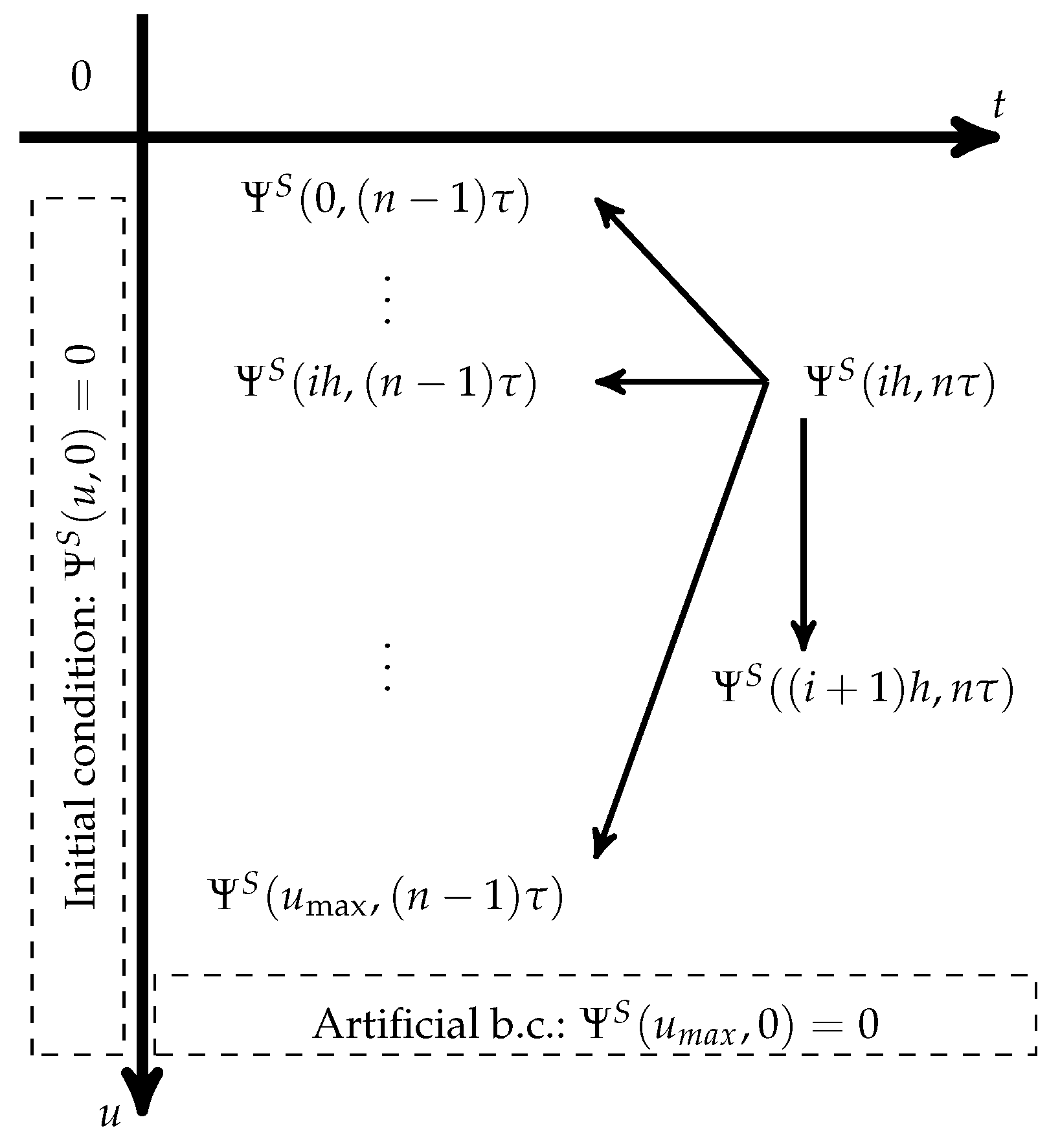
See Figure 1 for a graphical illustration of the dependence structure of the scheme. We can see that (7) is a semi-implicit approximation of (6) and on .
Regarding the stability of the scheme, we present the following estimate in the energy norm.
Lemma 1.
Let and let
Then, there is a constant C independent of and K such that for any
Proof.
Note that . Using Young’s inequality, we sum over and multiply by . We use the boundary condition to obtain:
Iterating the above estimate and noting that , we obtain
□
4.2. Numerical Experiments Verifying Convergence
We will use Remark 2 to obtain an analytical solution to (6). This can be compared to numerical approximations of the solution to verify convergence. The numerical method can then be applied for other distributions of claim size . The constants used in the numerical experiments are in Table 1.
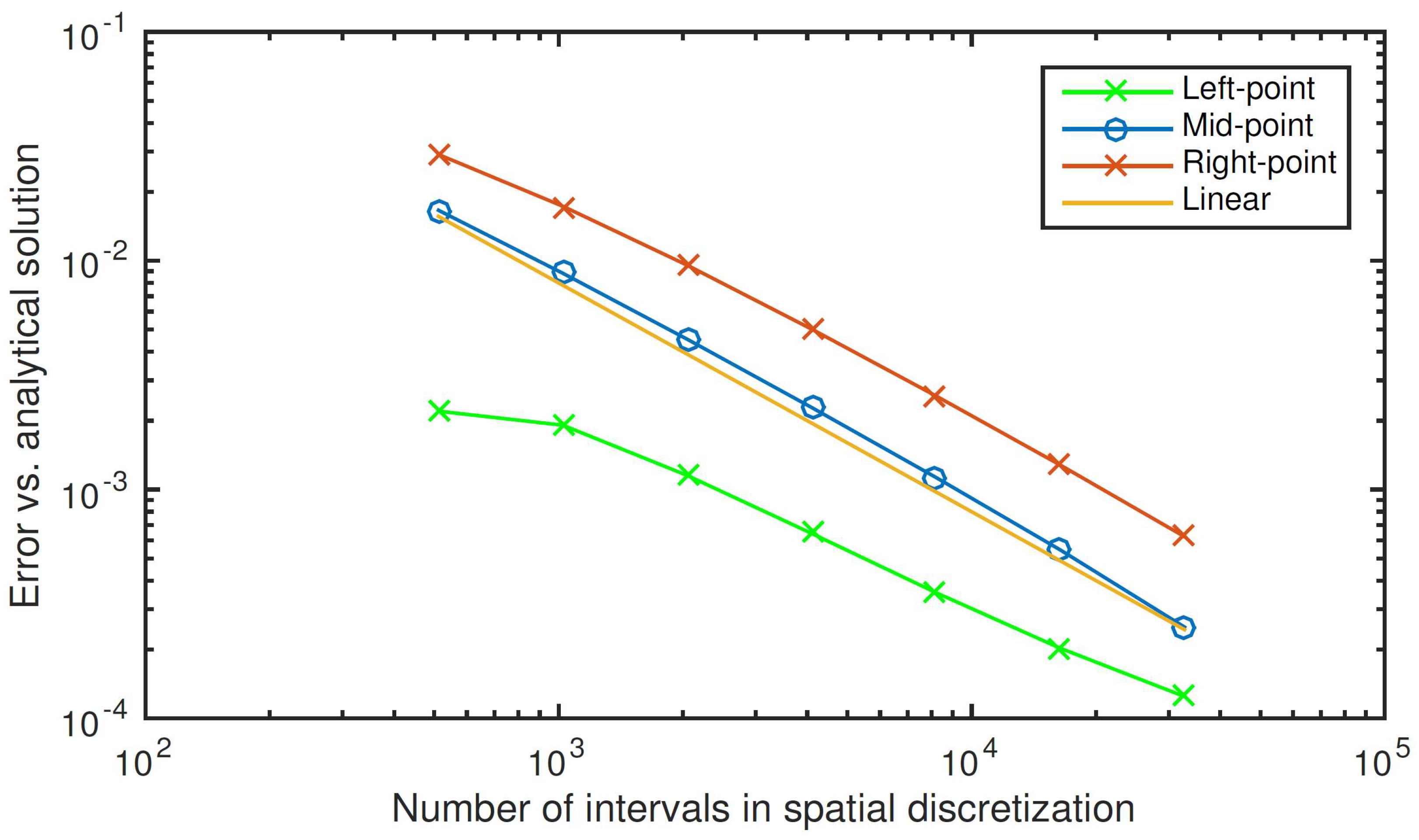
Figure 2 demonstrates the convergence of approximation with different schemes as with other parameters fixed. One observes that as the number of space steps increases, all three methods converge.
4.3. Results for Finite-TIME Ruin Probability
Until now, we have analysed the stability and checked the convergence of the numerical scheme. In this section, some by-products of our algorithm will be introduced. One advantage of applying the finite-difference method is that we will have the dynamics of the PDE system when we solve it. We are not yet applying in this section the algorithm to calculate the ruin probability under the stop-loss reinsurance setting.
Instead of solving a single setting of ruin probability directly, we separate the time horizon into many small time intervals, and this actually provides us additional information about the ruin process with respect to the time at least when the grid size is chosen large enough. For each of the s, we approximated inside the process until reaching the final . We also approximate how ruin probability will behave in each of these finite-time horizons (with accuracy decreasing while n becomes smaller). The same by-product also comes when we divide the initial capital u into segments. These by-products can be justified by the deterministic property of the PDE system, as in Equation (6). If the arguments of reaching a decent accuracy when approximating a via this scheme stand, then one can say that any where and can be approximated to the same accuracy. Thus, in one run, a large enough grid size can be found to approximate with the required accuracy.
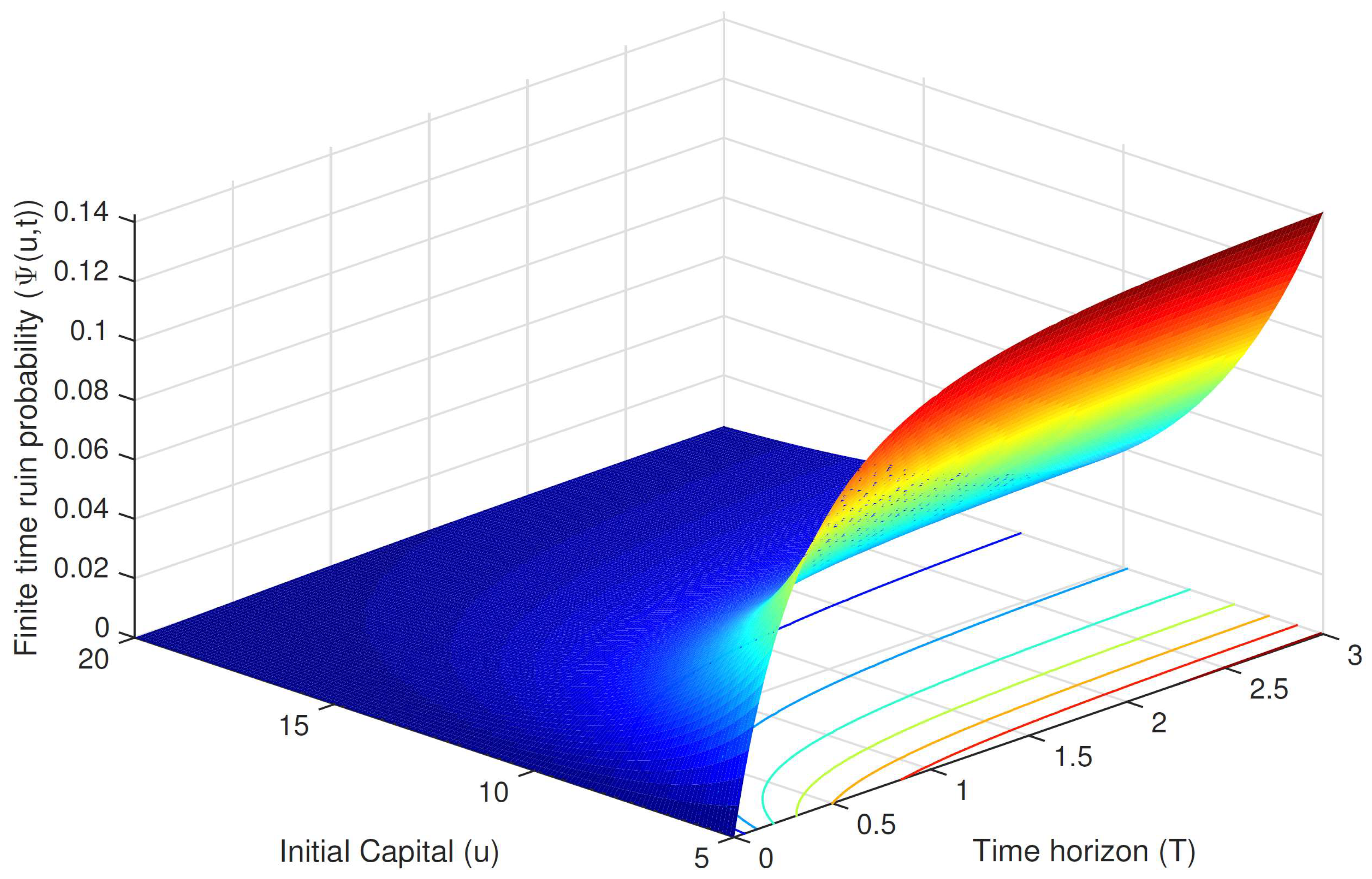
One can also study the dynamics of finite-time ruin probability more directly by iterating our algorithm on several where and . Figure 5 gives a comprehensive view of how the finite-time ruin probability varies as a function of the initial capital u and time horizon T1. One can observe that the finite-difference method approximation gives a ruin probability that increases as the time horizon increases and decreases as the initial capital increases, as expected.
We can also analyse the finite-time ruin probability under different parameter settings. By changing the initial capital u, premium rate c, Poisson intensity , and claim average size separately, we can analyse the behaviour of the finite-time ruin probabilities as well as compare these with the infinite-time ruin probability. As one can see from Table 2, the finite-time ruin probabilities increase with time and converge to the infinite-time ruin probability in all settings we have considered. We can further confirm that the numerical method is working as it should as the approximate ruin probability increases with claims intensity and claim average size, and decreases when initial capital and premium rate increases.
5. Finite-Time Ruin Probability with and without Stop-Loss Reinsurance
A direct application of the above algorithm is to calculate the finite and infinite-time ruin probability when stop-loss reinsurance is considered. For simplicity, in this study, we assume that the premium for the reinsurance contract is determined by the pure risk premium principle. By definition, the pure premium principle allocates to the reinsurer a certain proportion of the difference between the expected claims and the retention level as its premium, i.e., , where (usually we have ) is the premium rate for reinsurance. Denote by the retention level of a stop-loss reinsurance contract with premium rate . Given the result in (3), determining the ruin probability under stop-loss reinsurance reduces itself to the finite-time ruin probability, i.e., , with the only parameter left unknown. However, as shown in Theorem 1, , with , where T is the length of the reinsurance contract.
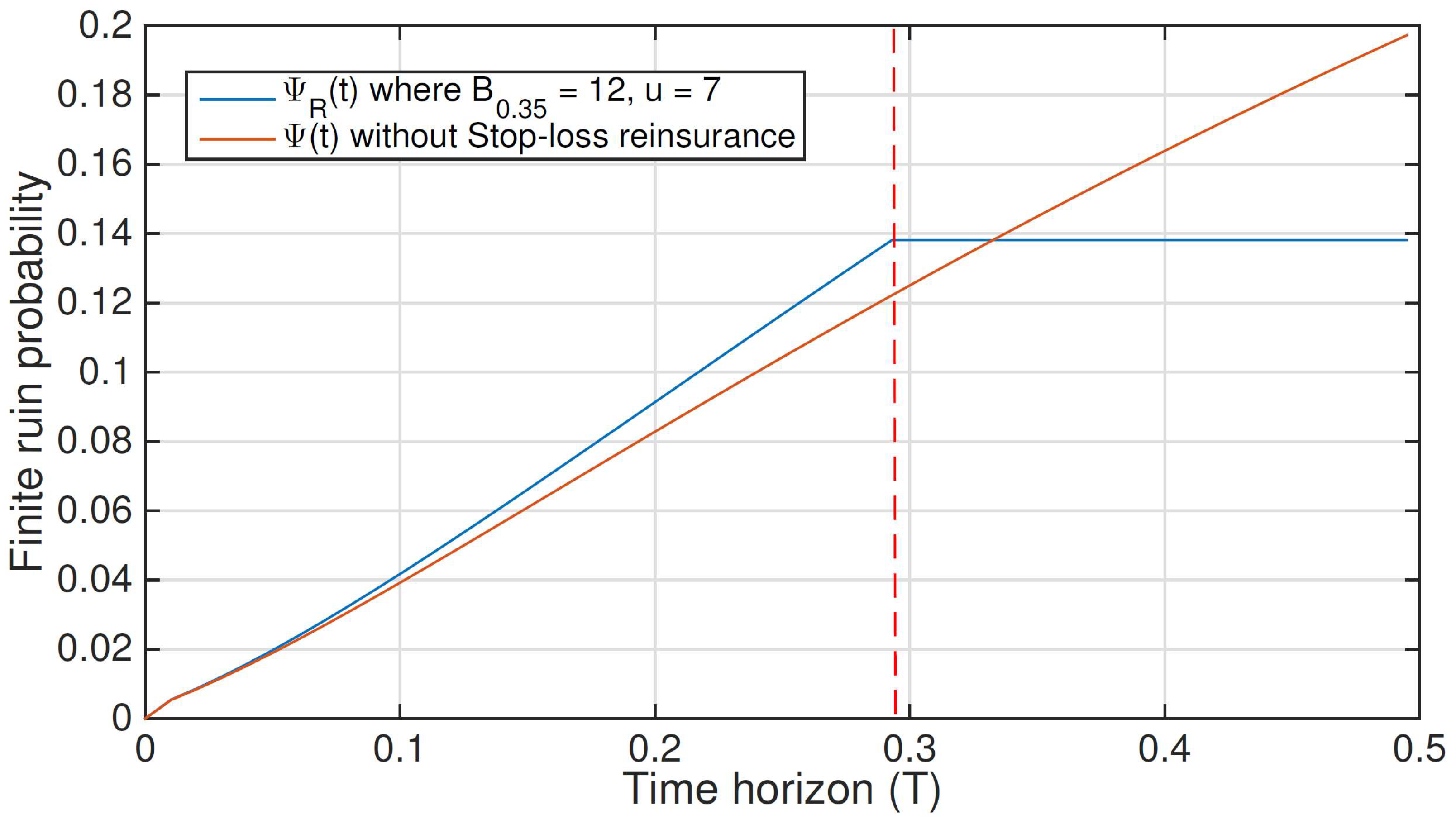
We can visualise the effect of buying stop-loss reinsurance on the ruin probability by plotting in Figure 6 the ruin probability for different time horizons, with and without reinsurance. Here, the stop-loss reinsurance contract is T years long. One can see from the plot that, up to a certain time horizon, the ruin probability with stop-loss reinsurance is larger than the ruin probability without stop-loss reinsurance. This can be explained by the costs associated with the reinsurance contract. Meanwhile, if the ceding company has not faced ruin before this particular time horizon, it will not face ruin probability for longer horizons, since the reinsurance is capping the claims to be paid. This feature that we observe here is consistent with the argument used in the proof of Theorem 2. Indeed, in the same figure, one can observe that the finite-time ruin probability will not increase for time horizons longer than marked by the red dashed line in the plot, the moment when the stop-loss reinsurance starts to pay claims. There is a time horizon such that, as expected, for horizons longer than that, the finite-time ruin probabilities are smaller when reinsurance is present.
6. Finite-Time Ruin Probability, Stop-Loss Retention Level and Initial Capital
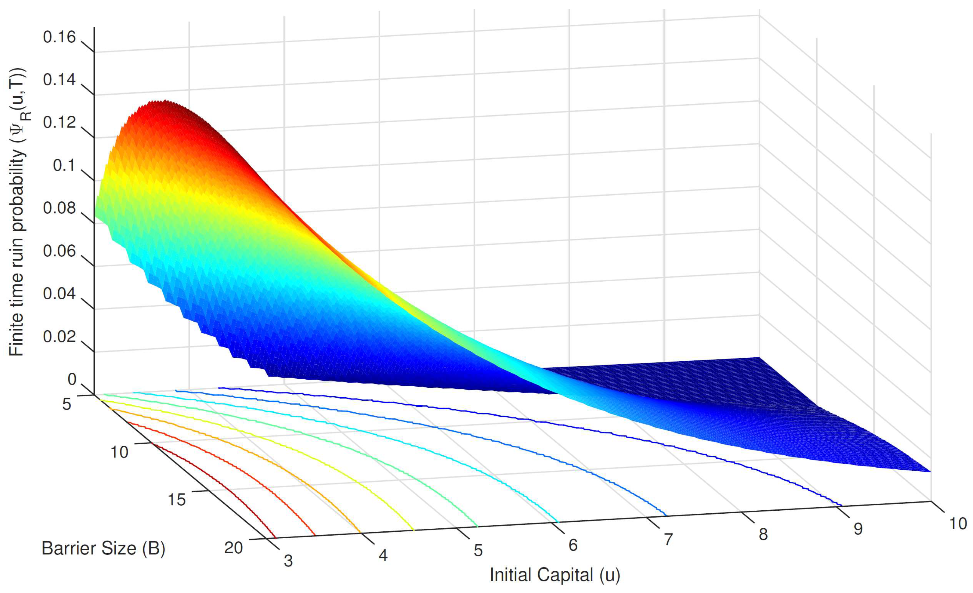
Next, we study the dynamics of the ceding company’s ruin probability under a stop-loss reinsurance contract. The 3-d graph in Figure 7 shows how initial capital u, and stop-loss retention level B affect the finite-time ruin probability. When the initial capital is large and the stop-loss retention level is small (corner further away in the plot), the ruin probability equals zero (i.e., there is no ruin). In fact, when the stop-loss retention level B is smaller than (or equal to) the initial capital u, we obtain from Theorem 1 that , and hence the probability of ruin is zero. Then, as the retention level increases, which indicates that the reinsurer takes fewer risks and the ceding company may face more risks itself, the ruin probability for the ceding company increases.
We can also observe in the plot that the reduction in the initial capital increases the ruin probability as we expected. We do not know exactly how ruin probability will behave without accurate parameter estimates and the exact reinsurance pricing mechanism. However, in the case studied here, the ceding company’s premium is relatively high; as a matter of fact, it is so high, that for longer time horizons, with the help from the reinsurance company, it will not face ruin. We can observe these finite-time ruin probability dynamics in Figure 7.
Moreover, Figure 7 tells us an even more interesting story, namely how the initial capital will compensate for the choice of stop-loss retention level, which, consequently, compensates for the cost of buying stop-loss reinsurance. Telling from the colour, choosing any fixed retention level, the increase in initial capital will drop the ruin probability, and for any fixed initial capital, the increase in retention level will boost the ruin probability up to some point. Moreover, the curves in the initial capital versus retention level plain, which help us tell the height of the surface, are actually a measure of how the initial capital compensates for the stop-loss retention level and thus ensure the efficiency of the stop-loss reinsurance contract.
For example, for relatively low initial capitals, say the high retention level and low initial capital corner, the small size of initial capital requires a small retention level of stop-loss reinsurance to keep it in the lower ruin probability region, i.e., the dark blue part. This small retention level of stop-loss reinsurance means an expensive contract, as the reinsurer takes more risks. On the other hand, with relatively large initial capitals, the ceding company can stay safe (i.e., small ruin probability) even with large retention levels, which means cheaper reinsurance contracts, but more risk for the ceding company. One sees here how initial capital and retention level compensate for each other. In reality, it all depends on the ceding company itself to choose between buying a more expensive reinsurance contract or just raising more capital (rather than spending on reinsurance).
Furthermore, one can easily observe that, whenever the company targets a certain ruin probability, as the retention level becomes larger, the increase on itself will compensate less and less for the increase in the initial capital, thus exhibiting “diminishing returns”. This indicates a low sensitivity of ruin probability to retention level when the latter is large.
7. Stop-Loss Reinsurance and The Primary Insurer Solvency
Risk of insolvency has sustained an increase in risk regulation for the insurance industry over the last decades. In the United States, the National Association of Insurance Commissioners supports the development of insurance regulations by individual states and has promoted the notion of risk-based capital for insurance companies. In Europe, the European Insurance and Occupational Pensions Authority oversees the development of the Solvency II framework. Under Solvency II, insurance companies must calculate their Solvency Capital Requirement, or Solvency II Economic Capital (EC), where all assets and liabilities should be valued on a market-consistent basis. According to this regulatory framework the EC ensures that the probability of insolvency over a one-year period does not surpasses 0.5%. To calculate their portfolio overall capital requirement, an insurance company must consider all the risks and their interactions. The methodology developed in this article can be used in the calculation of the capital requirement for a homogeneous insurance segment. According to Solvency II, the capital requirement for the all insurance company can then be calculated using an internal model or a simpler standard formula where the aggregation of risks is done using correlation parameters. A discussion of the aggregation properties of the two different approaches is out of the scope of this article.
From a risk measurement perspective, the EC, being an estimate of the capital necessary to keep the probability of insolvency below 5%, can be calculated as the one-year market-value based value-at-risk (VaR). In our framework, we take the initial capital corresponding to a one-year horizon ruin probability of 0.5% as the required EC. By simulation and interpolation of the results from our algorithm, we can calculate the initial capital corresponding to a ruin probability of 0.5% with a one-year time horizon. The results are in Table 3.
In panel A, we list, for different parameter values and when there is no reinsurance contract in place, the value of the initial capital corresponding to a 0.5% ruin probability for a time horizon ranging from about 5 weeks to 8 years. The initial capital necessary to maintain the desired level of ruin probability increases with the average aggregate claims and decreases when the premium rate increases. In panel B we list, for two values of reinsurer premium rates, the value of the initial capital corresponding to a 0.5% ruin probability for a one-year time horizon when there is a stop-loss reinsurance contract in place. We observe that reinsurance substantially lowers the amount of initial capital (economic capital) required in relation to the no-reinsurance case. Interestingly, once there is a stop-loss reinsurance contract in place, increasing the reinsurance premium rate from to does not increase the required initial capital that much when compared with the significant reduction implied by the introduction of reinsurance.
8. Conclusions
We employ ruin probability as a measure of the risk of an insurance company solvency. We propose a relationship between the finite and infinite-time ruin probability for a portfolio with stop-loss reinsurance and the finite-time ruin probability for a portfolio with no reinsurance contract. This can be found in Theorem 1. According to Remark 1, ruin would never happen for a time horizon longer than a certain for a portfolio with stop-loss reinsurance, which is illustrated in Figure 2. When employing aggregate stop-loss reinsurance, we build on two novel approaches: firstly, the connection introduced here between the finite and infinite-time ruin probability of a stop-loss portfolio and the finite-time ruin probability of a classical reinsurance free portfolio, and secondly, on the adaptation of the finite-difference method normally used for solving partial differential equations to solve the integro-partial differential equation the finite-time ruin satisfies. With the results at hand, a risk analysis is performed, identifying the combination of initial capital and retention level for which ruin is no longer possible, the diminishing returns of the balancing of initial capital and retention level and, not last, the variations on solvency for different time horizons. Analysing these dynamics between the parameters involved proves relevant to the risk management of an insurance portfolio. The methodology presented in this article allows us to identify the level of the primary insurer capital and corresponding retention level under a stop-loss contract necessary to keep a desired low level of insolvency risk. By entering in a stop-loss contract, the primary insurer can significantly reduce the capital without increasing the level of insolvency risk. In most cases, employing reinsurance is always better than not in terms of ruin probabilities and solvency capital requirements.
Author Contributions
Conceptualization, C.C., A.D., B.L., D.Š. and S.W.; methodology, C.C., A.D., B.L., D.Š. and S.W.; formal analysis, C.C., A.D., B.L., D.Š. and S.W.; writing, C.C., A.D., B.L., D.Š. and S.W. All authors have read and agreed to the published version of the manuscript.
Funding
Funding was received from the Casualty Actuarial Society, Constantinescu LOA 2014 (USD 10,800).
Data Availability Statement
Not applicable.
Acknowledgments
The authors would like to express their gratitude for the support provided by the Casualty Actuarial Society in completing this research.
Conflicts of Interest
The funders had no role in the design of the study; in the collection, analyses, or interpretation of data; in the writing of the manuscript, or in the decision to publish the results.
| 1 | Note the difference between Figure 5 and Figure 7. In here, we present how time horizon affects ruin probability, which is not the same concept as how big is the retention level of stop-loss reinsurance. Referring to the formula linking the critical time and the retention level B, we can see that the retention level is a function of time and initial capital; since we are changing both of these parameters here, each point on this surface represents a different retention level, which results in a different story of how stop-loss affects ruin probability. |
References
- Albrecher, Hansjörg, Corina Constantinescu, Gottlieb Pirsic, Georg Regensburger, and Markus Rosenkranz. 2010. An algebraic operator approach to the analysis of Gerber—Shiu functions. Insurance: Mathematics and Economics 46: 42–51. [Google Scholar] [CrossRef] [Green Version]
- Albrecher, Hansjörg, Jan Beirlant, and Jozef L. Teugels. 2017. Reinsurance: Actuarial and Statistical Aspects. Wiley Series in Probability and Statistics; Hoboken: John Wiley & Sons. [Google Scholar]
- Arrow, Kenneth J. 1963. Uncertainty and the welfare economics of medical care. The American Economic Review 53: 941–73. [Google Scholar]
- Asmussen, Soren, and Hansjorg Albrecher. 2010. Ruin Probabilities. In Advanced Series on Statistical Science & Applied Probability. River Edge: World Scientific Publishing Co., Inc. [Google Scholar]
- Borch, Karl. 1975. Optimal insurance arrangements. Astin Bulletin 8: 284–90. [Google Scholar] [CrossRef] [Green Version]
- Gajek, Lesław, and Dariusz Zagrodny. 2004. Reinsurance arrangements maximizing insurer’s survival probability. Journal of Risk and Insurance 71: 421–35. [Google Scholar] [CrossRef]
- Guerra, Manuel, and Maria de Lourdes Centeno. 2008. Optimal reinsurance policy: The adjustment coefficient and the expected utility criteria. Insurance: Mathematics and Economics 42: 529–39. [Google Scholar] [CrossRef]
- Guerra, Manuel, and Maria de Lourdes Centeno. 2010. Optimal reinsurance for variance related premium calculation principles. Astin Bulletin 40: 97–121. [Google Scholar] [CrossRef] [Green Version]
- Haas, Sandra. 2012. Optimal Reinsurance Forms and Solvency. Ph.D. thesis, Université de Lausanne, Switzerland. [Google Scholar]
- Kull, Andreas. 2009. Sharing risk—An economic perspective. Astin Bulletin 39: 591–613. [Google Scholar] [CrossRef] [Green Version]
- Pervozvansky, A. A. 1998. Equation for survival probability in a finite time interval in case of non-zero real interest force. Insurance: Mathematics and Economics 23: 287–95. [Google Scholar] [CrossRef]
- Pesonen, Martti. 1984. Optimal reinsurances. Scandinavian Actuarial Journal 2: 65–90. [Google Scholar] [CrossRef]
- Rolski, Tomasz, Hanspeter Schmidli, Volker Schmidt, and Jozef L. Teugels. 1999. Stochastic Processes for Insurance and Finance. Chichester: John Wiley & Sons Ltd. [Google Scholar]
Figure 1.
Scheme dependence diagram.

Figure 2.
Convergence using different S for approximating the convolution term. We note that for mid-point and right–point schemes, the convergence is clearly linear. For the left-point scheme, it appears to be sub–linear.
Figure 2.
Convergence using different S for approximating the convolution term. We note that for mid-point and right–point schemes, the convergence is clearly linear. For the left-point scheme, it appears to be sub–linear.

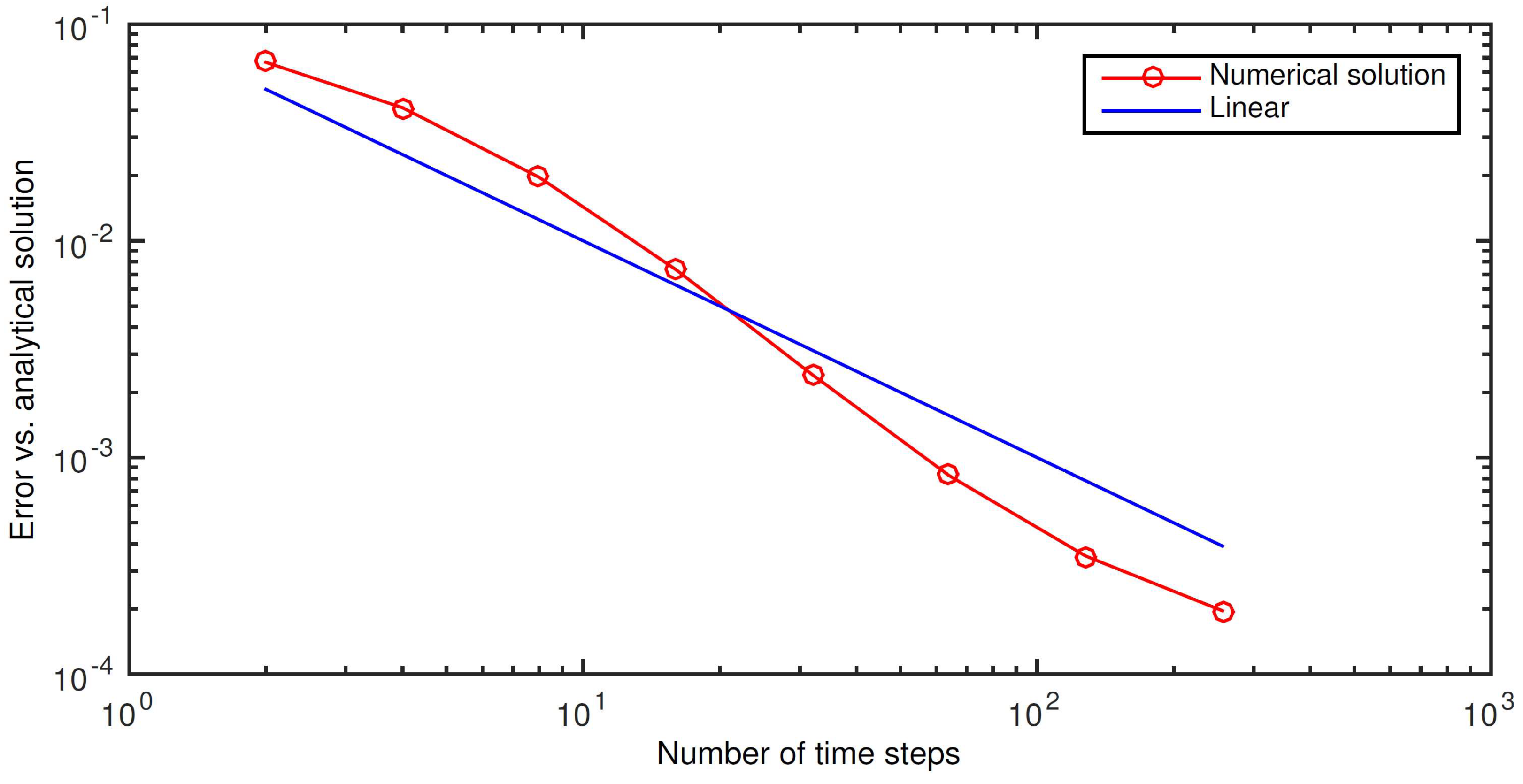
Figure 3.
Convergence as . We note that the convergence appears to be linear.

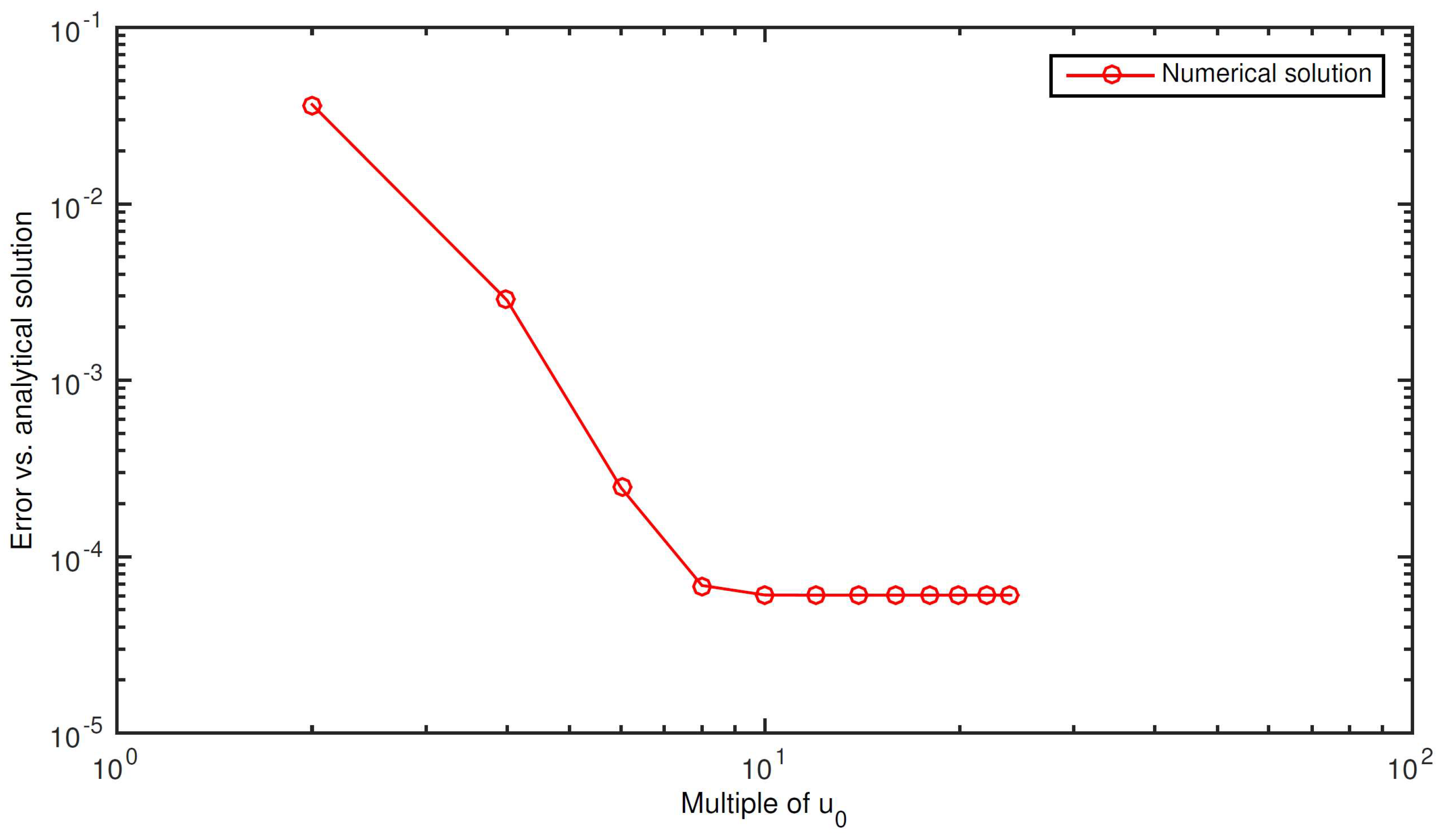
Figure 4.
Convergence as . Here, the convergence is exponential. It appears that K of 10 already produces errors of order in the ruin probability, and the choice of and h are the determining factors for producing the required accuracy.
Figure 4.
Convergence as . Here, the convergence is exponential. It appears that K of 10 already produces errors of order in the ruin probability, and the choice of and h are the determining factors for producing the required accuracy.

Figure 5.
Plot of finite-time ruin probability: this is a numerical approximation showing how the initial capital and the time horizon affect the finite-time ruin probability. Initial capital varies from 10 to 20, time horizon ranges from 0 to 3, , , , and other parameters are as in Table 1.
Figure 5.
Plot of finite-time ruin probability: this is a numerical approximation showing how the initial capital and the time horizon affect the finite-time ruin probability. Initial capital varies from 10 to 20, time horizon ranges from 0 to 3, , , , and other parameters are as in Table 1.

Figure 6.
Finite-time ruin probability with and without stop-loss reinsurance.

Figure 7.
Plot of finite-time ruin probability with stop-loss reinsurance: this is a numerical approximation showing how initial capital and stop-loss retention level influence finite-time ruin probability. Initial capital varies from 3 to 10, the retention level from 5 to 20, , , , and all other parameters are as in Table 1.


Table 1.
Constants used in the numerical experiments: is the (finite) time horizon, c is the premium rate, is the claim intensity, is the mean claim size and is the largest initial capital for which we wish to approximate the probability of ruin in finite time.
Table 1.
Constants used in the numerical experiments: is the (finite) time horizon, c is the premium rate, is the claim intensity, is the mean claim size and is the largest initial capital for which we wish to approximate the probability of ruin in finite time.
| Parameter | T | c | |||
| Value | 5 | 5 | 20 | 5 | 0.5 |
Table 2.
Finite and infinite-time ruin probability under different parameter settings. For the parameters, u is the initial capital, c is the premium rate, is the claim intensity, and is the mean claim size.
Table 2.
Finite and infinite-time ruin probability under different parameter settings. For the parameters, u is the initial capital, c is the premium rate, is the claim intensity, and is the mean claim size.
| Parameters | Time Horizon, T (Years) | ||||||
|---|---|---|---|---|---|---|---|
| 0.1 | 0.5 | 1 | 2 | 4 | 8 | Infinity | |
| (5, 20, 5, 0.5) | 0.035165 | 0.099974 | 0.125627 | 0.139186 | 0.142946 | 0.143313 | 0.143252 |
| (5, 15, 5, 0.5) | 0.039238 | 0.137707 | 0.195929 | 0.244954 | 0.275293 | 0.287726 | 0.289732 |
| (5, 20, 7, 0.5) | 0.053630 | 0.174861 | 0.238538 | 0.288632 | 0.318013 | 0.329485 | 0.330657 |
| (5, 20, 5, 0.3) | 0.095225 | 0.287057 | 0.391502 | 0.484876 | 0.557218 | 0.606357 | 0.649001 |
| (10, 20, 5, 0.5) | 0.004292 | 0.020611 | 0.031224 | 0.038415 | 0.040771 | 0.041025 | 0.041042 |
| (10, 15, 5, 0.5) | 0.004855 | 0.031306 | 0.058143 | 0.088889 | 0.112544 | 0.123639 | 0.125917 |
| (10, 20, 7, 0.5) | 0.007359 | 0.046122 | 0.081174 | 0.117582 | 0.143278 | 0.154477 | 0.156191 |
| (10, 20, 5, 0.3) | 0.027800 | 0.128481 | 0.211560 | 0.303877 | 0.386723 | 0.448424 | 0.505442 |
Table 3.
Initial capital corresponding to a 0.5% ruin probability for different parameter values of the risk process. For the parameters, c is the insurer premium rate, is the claim intensity, is the mean claim size, and is the reinsurer premium rate.
Table 3.
Initial capital corresponding to a 0.5% ruin probability for different parameter values of the risk process. For the parameters, c is the insurer premium rate, is the claim intensity, is the mean claim size, and is the reinsurer premium rate.
| Panel A: Without Reinsurance | ||||||
|---|---|---|---|---|---|---|
| Parameters | Time Horizon, (Years) | |||||
| 0.1 | 0.5 | 1 | 2 | 4 | 8 | |
| (20, 5, 0.5) | 9.593921 | 14.188087 | 16.232585 | 17.713893 | 18.320151 | 18.405424 |
| (15, 5, 0.5) | 9.893007 | 15.643934 | 19.054614 | 22.792824 | 26.261153 | 28.565091 |
| (20, 7, 0.5) | 10.857631 | 17.401518 | 21.315918 | 25.605376 | 29.565199 | 32.094999 |
| (20, 5, 0.3) | 16.802917 | 27.698801 | 34.573297 | 40.518959 | 46.216685 | 52.393767 |
| Panel B: With Reinsurance and | ||||||
| Retention Level, | ||||||
| 1 | 2 | 4 | 6 | 8 | 10 | |
| (20, 5, 0.5) | 3.532088 | 3.521673 | 3.500712 | 6.379115 | 4.432340 | 11.204400 |
| (15, 5, 0.5) | 3.699426 | 3.689711 | 3.670160 | 6.463373 | 3.168102 | 10.553199 |
| (20, 7, 0.5) | 4.997532 | 4.994197 | 4.987510 | 5.584031 | 3.922885 | 8.700725 |
| (20, 5, 0.3) | 7.370037 | 7.367306 | 7.361851 | 7.357099 | 7.292685 | 6.793047 |
| (20, 5, 0.5) | 3.712315 | 3.683212 | 3.623897 | 6.436518 | 4.343473 | 11.204400 |
| (15, 5, 0.5) | 3.867475 | 3.840345 | 3.785043 | 6.474379 | 2.375872 | 10.553199 |
| (20, 7, 0.5) | 5.082380 | 5.072757 | 5.053388 | 5.607053 | 3.322549 | 6.186034 |
| (20, 5, 0.3) | 7.456775 | 7.448370 | 7.431625 | 7.415705 | 7.327712 | 6.533600 |
Publisher’s Note: MDPI stays neutral with regard to jurisdictional claims in published maps and institutional affiliations. |
© 2022 by the authors. Licensee MDPI, Basel, Switzerland. This article is an open access article distributed under the terms and conditions of the Creative Commons Attribution (CC BY) license (https://creativecommons.org/licenses/by/4.0/).
Share and Cite
MDPI and ACS Style
Constantinescu, C.; Dias, A.; Li, B.; Šiška, D.; Wang, S. Effect of Stop-Loss Reinsurance on Primary Insurer Solvency. Risks 2022, 10, 193. https://doi.org/10.3390/risks10100193
AMA Style
Constantinescu C, Dias A, Li B, Šiška D, Wang S. Effect of Stop-Loss Reinsurance on Primary Insurer Solvency. Risks. 2022; 10(10):193. https://doi.org/10.3390/risks10100193
Chicago/Turabian StyleConstantinescu, Corina, Alexandra Dias, Bo Li, David Šiška, and Simon Wang. 2022. "Effect of Stop-Loss Reinsurance on Primary Insurer Solvency" Risks 10, no. 10: 193. https://doi.org/10.3390/risks10100193
Note that from the first issue of 2016, this journal uses article numbers instead of page numbers. See further details here.