
Fricke Topological Qubits


1
Institut FEMTO-ST CNRS UMR 6174, Université de Bourgogne/Franche-Comté, 15 B Avenue des Montboucons, F-25044 Besançon, France
2
Quantum Gravity Research, Los Angeles, CA 90290, USA
*
Author to whom correspondence should be addressed.
†
These authors contributed equally to this work.
Quantum Rep. 2022, 4(4), 523-532; https://doi.org/10.3390/quantum4040037
Submission received: 7 October 2022
/
Revised: 1 November 2022
/
Accepted: 9 November 2022
/
Published: 14 November 2022
(This article belongs to the Special Issue Exclusive Feature Papers of Quantum Reports)
Abstract
:We recently proposed that topological quantum computing might be based on representations of the fundamental group for the complement of a link K in the three-sphere. The restriction to links whose associated character variety contains a Fricke surface is desirable due to the connection of Fricke spaces to elementary topology. Taking K as the Hopf link , one of the three arithmetic two-bridge links (the Whitehead link , the Berge link or the double-eight link ) or the link , the for those links contains the reducible component , the so-called Cayley cubic. In addition, the for the latter two links contains the irreducible component , or , respectively. Taking to be a representation with character (), with , then fixes a unique point in the hyperbolic space and is a conjugate to a representation (a qubit). Even though details on the physical implementation remain open, more generally, we show that topological quantum computing may be developed from the point of view of three-bridge links, the topology of the four-punctured sphere and Painlevé VI equation. The 0-surgery on the three circles of the Borromean rings L6a4 is taken as an example.
1. Introduction
Building a quantum computer is still challenging. However, progress has been made using natural and artificial atoms [1], superconducting technology [2] and other physical techniques [3,4]. One of the greatest challenges involved with constructing quantum computers is controlling or removing quantum decoherence. One possible solution is to create a topological quantum computer.
The paper describes progress towards an understanding and possibly an implementation of quantum computation based on algebraic surfaces. In the orthodox acceptation, a topological quantum computer deploys two-dimensional quasiparticles called anyons that are braids in three dimensions. The braids lead to logic gates used for computation. The topological nature of the braids makes the quantum computation less sensitive to the decoherence errors than in a standard quantum computer [5,6]. One theoretical proposal of universal quantum computation is based on Fibonacci anyons that are non-Abelian anyons with fusion rules. In particular, a fractional quantum Hall device would, in principle, realize a topological qubit. Owing to the lack of evidence that such quantum Hall-based anyons have been obtained, other theoretical proposals are worthwhile to develop. A recent paper of our group proposed a correspondence between the fusion Hilbert space of Fibonacci anyons and the tiling two-dimensional space of the one-dimensional Fibonacci chain [7].
In this paper, following our recent proposal [8] (see also [9]), we propose a non-anyonic theory of a topological quantum computer based on surfaces in a three-dimensional topological space. Such surfaces are part of the character variety underlying the symmetries of a properly chosen manifold. In our earlier work, we were interested in basing topological quantum computing on three- or four-manifolds defined from the complement of a knot or link. In [10,11], our goal was to define informationally complete quantum measurements from three-manifolds and, in [12], from four-manifolds, seeing the embedding four-dimensional ‘exotic’ space of the manifold as a the physical Euclidean space-time. In the later paper, exotism means that one can define homeomorphic but non-diffeomorphic four-dimensional manifolds to interpret a type of ‘many-world’ quantum measurements.
Our concepts in [8] and in the present paper are different in the sense that the character variety is the three-dimensional locus of the supposed qubit prior to its measurement. The Lorentz group reads the symmetries of the selected topology like that of the punctured torus, the quadruply punctured sphere or the topology obtained from the complement of a knot or a link. Our work in [8] focused on the complement of the Hopf link—the linking of two unknotted curves—where the character variety consists of the Cayley cubic . Here, we took the broader context of Fricke surfaces, whose compact bounded component consists of the representations [13]. Such representations are our proposed model of the topological qubits.
In Section 2, we recall the definition of the -character variety for a manifold M whose fundamental group is and the method used to build it in an explicit way.
In Section 3, we focus on the character variety for the fundamental group (the free group of rank 2) of the once-punctured torus and on the character variety attached to the fundamental group of the Hopf link L2a1. The former case is found to be related to the two-bridge link . The role of the extended mapping class group on a character variety of type , , is emphasized. We also introduce the concept of a topological qubit associated to the bounded component of the surface .
In Section 4, we focus on the character variety for the fundamental group (the free group of index 3) of the quadruply punctured sphere . In particular, we recall the conditions that separate the compact (and bounded) component and the non-compact component. The investigation of the coverings of the four-manifold (the Kodaira singular fiber ) allows for an application of the theory. In the same section, we describe the Riemann–Hilbert correspondence for the case of , as well as the so-called Painlevé-Okomoto correspondence. The Painlevé VI equation plays a special role.
In Section 5, we apply some perspectives of the present research toward topological quantum computing related to cosmology.
2. The -Character Variety of a Manifold
Let be the fundamental group of a topological surface S. We describe the representations of in the Lorentz group , the group of matrices with complex entries and determinant 1. Such a group contains representations as degrees of freedom for all quantum fields and is the gauge group for the Einstein–Cartan theory, which contains the Einstein–Hilbert action and Einstein’s field equations [14]. Topological formulations of gravity have been introduced [15,16,17] and the relationship of entanglement with spacetime has been articulated [18,19], which motivates the exploration of character varieties for quantum computation.
Representations of in are homomorphisms with character , . The set of characters allows us to define an algebraic set by taking the quotient of the set of representations by the group , which acts by conjugation on representations [13,20].
Below, we need the distinction between the two real forms and of the group . The representations are those that fix a point in the three-dimensional hyperbolic space and representations are those that preserve a two-dimensional hyperbolic space in , as well as an orientation of . Both real forms of play an important role in our attempt to define and stabilize the potential Fricke topological qubits.
A Sage Program for Computing the -Character Variety of
The SL character variety of a manifold M defined in SnapPy may be calculated in Sage using a program [21] written by the last author of [20] as follows:
from snappy import Manifold
M = Manifold(‘M’)
G = M.fundamental_group()
I = G.character_variety_vars_and_polys(as_ideal=True)
I.groebner_basis()
In some cases, a Groebner basis is not obtained from Sage. One may also use Magma [22] to obtain the Groebner basis or a small basis with the shortest length of the ideal I.
3. The Cubic Surface and Two-Bridge Links
Following [23], in this section, we describe the special case of representations for the punctured torus and the relevance of the extended mapping class group in its action on surfaces of type , . Then, we find that surfaces and are contained in the character variety for the fundamental group of links L7a4 and L6a1, respectively. The representations and the concept of a Fricke topological qubit is outlined.
3.1. The -Character Variety for a Once Punctured Torus
Let us take the example of the punctured torus whose fundamental group is the free group on two generators a and b. The boundary component of is a single loop around the puncture expressed by the commutator with and . We introduce the traces
Another noticeable surface is obtained from the character variety attached to the fundamental group of the Hopf link that links two unknotted curves. For the Hopf link, the fundamental group is
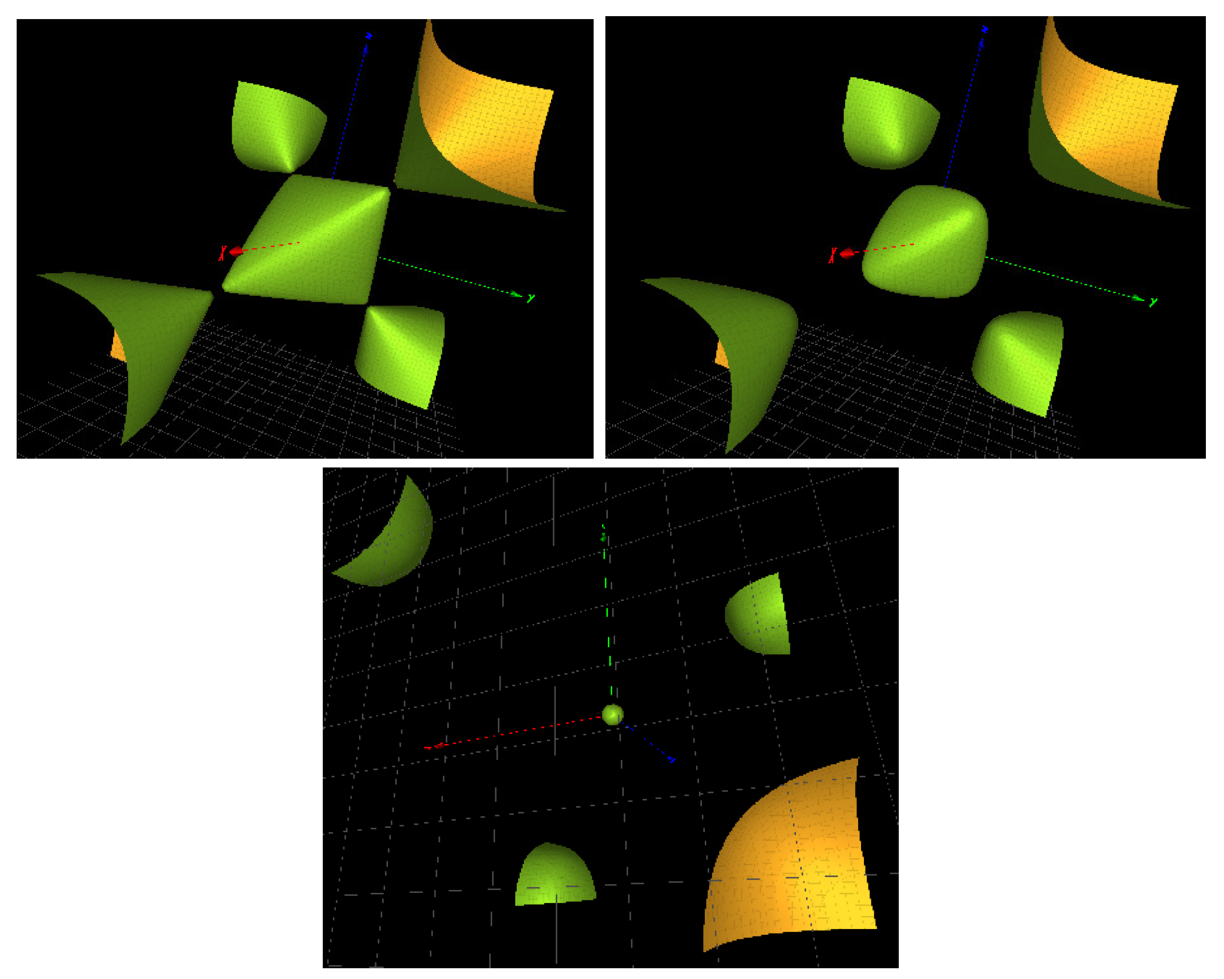
and the corresponding character variety is the Cayley cubic [8]
Both surfaces and are shown in Figure 1.
Surfaces and have been obtained from two different mathematical concepts, from topological and algebraic concepts in dimension two, respectively. To relate them, one makes use of the Dehn–Nielsen–Baer theorem applied to the once-punctured torus [24]. According to this theorem, for a surface of genus , we have
where the mapping class group denotes the group of isotopy classes of orientation-preserving diffeomorphisms of S (that restrict to the identity on the boundary if ), the extended mapping class group denotes the group of isotopy classes of all homeomorphisms of S (including the orientation-reversing ones) and denotes the outer automorphism group of . This leads to the (topological) action of on the punctured torus as follows:
The automorphism group acts by composition on the representations and induces an action of the extended mapping class group on the character variety by polynomial diffeomorphisms of the surface defined by [25]
3.2. The Surface , the Link and Fricke Topological Qubits
The surface corresponds to representations of the group ([25] Section 4.2)
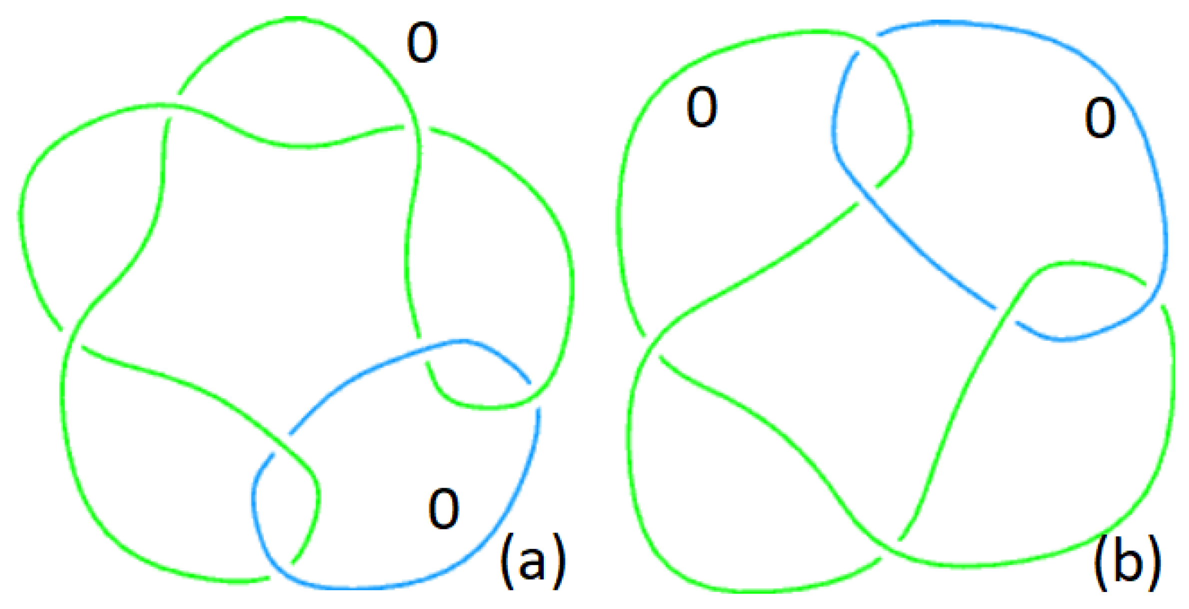
Since the surface is the character variety of the Hopf link, we would also like to obtain a link whose character variety contains the surface . Making use of the Thistlethwaite link table [26], we find that the only two-bridge link that has this property is the link ; see Figure 2. Taking 0-surgery on both cusps of , Snappy calculates the fundamental group as
The corresponding Groebner base for the character variety is
whose factorization contains both surfaces and .
Topological Qubits from
Qubits are the elements of group . There is an interesting connection of the group in Equation (3) to representations.
According to [25] [Theorem 1.1], there exists a representation such that the closure of the orbit of its conjugacy class under the action of the extended mapping class group in Equation (1) contains the whole set of representations of . The subset of the real surface consisting of representations is the unique bounded connected component of homeomorphic to a sphere; see Figure 1 (Right).
The bounded component is invariant under the mapping class and there are two fixed points of the polynomial transformation made of points with irrational values and ([25], p. 19).
3.3. The Surface and the Link
We would like to obtain a link whose character variety contains the surface . Making use of the Thistlethwaite link table [26], we find that the only two-bridge link that has this property is the link ; see Figure 2. Taking 0-surgery on both cusps of , Snappy calculates the fundamental group as
The corresponding Groebner base for the character variety is
whose factorization contains surface and a ninth-order trivariate polynomial not made explicit here.
4. The Fricke Cubic Surface and Three-Bridge Links
Our main object in this section is the four-punctured sphere , for which, the fundamental group is the free group of rank three whose character variety generalizes the Fricke cubic surface (2) to the hypersurface in . It is shown how this hypersurface is realized in the variety of a covering of index 6 of the four-manifold , the 0-surgery on all circles of the Borromean rings . The Okamoto–Painlevé correspondence is re-examined in terms of Dynkin diagrams of the appropriate four-manifolds.
4.1. The -Character Variety for the Quadruply Punctured Sphere
The fundamental group for can be expressed in terms of the boundary components A, B, C and D as .
A representation is a quadruple
Let us associate the seven traces
where a, b, c and d are boundary traces and x, y and z are traces of elements , and representing simple loops on .
4.2. A Compact Component of
As shown in the previous section, for the real surface , the compact component is made of representations.
For the real surface , there exists a compact component if and only if [27], Proposition 1.4
4.3. The Character Variety for the Manifold and for Its Covering Manifolds
In a recent paper ([8], Section 3.2), we noticed connections between the coverings of the manifold and the matter of topological quantum computing. The affine Coxeter–Dynkin diagram corresponds to the fiber in Kodaira’s classification of minimal elliptic surfaces ([30], p. 320). Alternatively, one can see as the 0-surgery on the trefoil knot . The boundary of the manifold associated to is the Seifert fibered toroidal manifold [31,32].
The coverings of the fundamental group are fundamental groups of the manifolds in the following sequence:
The subgroups/coverings are fundamental groups for , or , where is the manifold obtained by 0-surgery on all circles of Borromean rings.
A Groebner base for the character variety of is
where the latter two factors are quadrics.
A Groebner base for the character variety of is
where is the character variety for the fundamental group of the Hopf link complement, and . A plot of the latter surfaces is in ([8], Figure 4). In the three-dimensional projective space, the two surfaces are birationally equivalent to a conic bundle and to the projective plane , respectively. Both show a Kodaira dimension zero characteristic of surfaces.
A Groebner base for the character variety of contains the five- dimensional hypersurface
which is close to (but different from) the Fricke form .
Finally, for , a Groebner base obtained from Magma contains 28 polynomials. However, a simpler small basis with 10 polynomials, like the size of I, is available. The ideal ring for is
where the seventh variable polynomial reads
and , , , .
Taking the new variable , the polynomial transforms into the Fricke form (4).
with and .
The missing term in (6) is a fifth-order polynomial.
4.4. Painlevé VI and the Riemann-Hilbert Correspondence
Equation (7) corresponds to a four-punctured sphere with four singular points and a monodromy group isomorphic to the free group on three-generators. The existence of a certain class of linear differential equations with such singular points and a monodromy group is known as Hilbert’s twenty first problem, the original setting of Riemann–Hilbert correspondence. For the present case of the four-punctured sphere, the searched differential (dynamical) equation is the sixth Painlevé equation (or Painlevé VI) [23]
with complex parameters . The Painlevé property is the absence of movable singular points. The essential singularities of all solutions of Equation (8) only appear when .
Analyzing the nonlinear monodromy of Painlevé VI leads to the relation between parameters a, b, c and d of the family of cubic surfaces given in (7) and parameters , of Painlevé VI equation ([29], Section 4.2):
The relation between the two classes of parameters has been found to be controlled by the so-called Okamoto–Painlevé pairs. The Painlevé equation corresponding to is Painlevé I, the Painlevé equation corresponding to is Painlevé II, the Painlevé equation corresponding to is Painlevé IV and the Painlevé equation corresponding to is Painlevé VI ([33] Table 1, [23] Section 9.1.2). These mathematical results fit our approach developed in the previous subsection.
Incidentally, the Painlevé equation corresponding to the manifold is Painlevé V. We find that the Groebner base for the character variety of contains the surface defined in Equation (2) (apart from trivial quadratic factors).
Finally, Painlevé III corresponds to one of the three types , or . We find that, for and , the character variety is trivial (up to quadratic factors), for , it is of type and, for , it is close (but different from the form , as for investigated in Section 4.3.
The Okamoto–Painlevé correspondence and the type of main factor in the related Groebner base is summarized in Table 1.
5. Discussion and Conclusions
In this paper, using the character variety of the punctured torus and of the quadruply punctured sphere , we focused on the interest in defining topological qubits from the cubic surface in (2) or in (4) in the compact bounded domain of real variables x, y and z. We explored the connection of such real surfaces to the character variety of some two- and three-bridge links. We pointed out their relationship to Painlevé VI transcendents through Okamoto Equation (9). While possible experimental directions remain open for further investigation, recent advances in the field are noteworthy [34,35,36,37].
Let us now add that there exists a link between Painlevé transcendents and Einstein’s equations of cosmology when the metric is chosen to be self-dual. The six Painlevé equations are ‘essentially’ equivalent to self-dual Yang–Mills equations with appropriate three-dimensional Abelian groups of conformal symmetries [38]. The symmetry groups are taken to be groups of conformal transformations of the complex Minkowski space–time with the metric
For Painlevé VI, the Higgs fields , , 1, t are valued functions of the time variable . The self-dual equations
with are equivalent to Painlevé VI with parameters calculated from the constant determinants of the and S ([38], p. 573). As a result, the Fricke surfaces that we investigated in this paper correspond to relevant solutions of self-dual Einstein’s equations.
Author Contributions
Conceptualization, M.P.; methodology, M.P. and M.M.A.; software, M.P.; validation, D.C., M.M.A. and K.I.; formal analysis, M.P. and D.C.; investigation, M.M.A., D.C. and M.M.A.; data curation, M.P.; writing—original draft preparation, M.P.; writing—review and editing, M.P. and M.M.A.; visualization, M.M.A.; supervision, M.P.; project administration, K.I.; funding acquisition, K.I. All authors have read and agreed to the published version of the manuscript.
Funding
This research received no external funding.
Informed Consent Statement
Not applicable.
Data Availability Statement
Data are available from the authors after a reasonable demand.
Conflicts of Interest
The authors declare no conflict of interest.
References
- Buluta, I.; Ashhab, S.; Nori, F. Natural and artificial atoms for quantum computation. Rep. Prog. Phys. 2011, 74, 104401. [Google Scholar] [CrossRef] [Green Version]
- Obada, A.S.F.; Hessian, H.A.; Mohamed, A.B.A.; Homid, A.H. A proposal for the realization of universal quantum gates via superconducting qubits inside a cavity. Ann. Phys. 2013, 334, 47–57. [Google Scholar] [CrossRef]
- Top 10 Quantum Computing Experiments of 2019. Available online: https://medium.com/swlh/top-quantum-computing-experiments-of-2019-1157db177611 (accessed on 1 November 2022).
- Timeline of Quantum Computing and Communication. Available online: https://en.wikipedia.org/wiki/Timeline_of_quantum_computing_and_communication (accessed on 1 November 2022).
- Topological Quantum Computer. Available online: https://en.wikipedia.org/wiki/Topological_quantum_computer (accessed on 1 January 2021).
- Pachos, J.K. Introduction to Topological Quantum Computation; Cambridge University Press: Cambridge, UK, 2012. [Google Scholar]
- Amaral, M.; Chester, D.; Fang, F.; Irwin, K. Exploiting anyonic behavior of quasicrystals for topological quantum computing. Symmetry 2022, 14, 1780. [Google Scholar] [CrossRef]
- Planat, M.; Aschheim, R.; Amaral, M.M.; Fang, F.; Chester, D.; Irwin, K. Character varieties and algebraic surfaces for the topology of quantum computing. Symmetry 2022, 14, 915. [Google Scholar] [CrossRef]
- Asselmeyer-Maluga, T. Topological quantum computing and 3-manifolds. Quantum Rep. 2021, 3, 153–165. [Google Scholar] [CrossRef]
- Planat, M.; Aschheim, R.; Amaral, M.M.; Irwin, K. Universal quantum computing and three-manifolds. Symmetry 2018, 10, 773. [Google Scholar] [CrossRef] [Green Version]
- Planat, M.; Aschheim, R.; Amaral, M.M.; Irwin, K. Group geometrical axioms for magic states of quantum computing. Mathematics 2019, 7, 948. [Google Scholar] [CrossRef] [Green Version]
- Planat, M.; Aschheim, R.; Amaral, M.M.; Irwin, K. Quantum computation and measurements from an exotic space-time R4. Symmetry 2020, 12, 736. [Google Scholar] [CrossRef]
- Goldman, W.M. Trace coordinates on Fricke spaces of some simple hyperbolic surfaces. In Handbook of Teichmüller Theory; European Mathematical Society: Zürich, Switzerland, 2009; Volume 13, pp. 611–684. [Google Scholar]
- Hehl, F.W.; von der Heyde, P.; Kerlick, G.D.; Nester, J.M. General relativity with spin and torsion: Foundations and prospects. Rev. Mod. Phys. 1976, 48, 393–416. [Google Scholar] [CrossRef] [Green Version]
- Yang, C.N. Integral Formalism for Gauge Fields. Phys. Rev. Lett. 1974, 33, 445, Erratum in Phys. Rev. Lett. 1975, 35, 1748. [Google Scholar] [CrossRef]
- MacDowell, S.W.; Mansouri, F. Unified geometric theory of gravity and supergravity. Phys. Rev. Lett. 1977, 38, 739–742, Erratum in Phys. Rev. Lett. 1977, 38, 1376. [Google Scholar] [CrossRef]
- Trautman, A. The geometry of gauge fields. Czechoslov. J. Phys. B 1979, B29, 107–116. [Google Scholar] [CrossRef]
- Ryu, S.; Takayanagi, T. Holographic derivation of entanglement entropy from AdS/CFT. Phys. Rev. Lett. 2006, 96, 181602. [Google Scholar] [CrossRef] [PubMed] [Green Version]
- Van Raamsdonk, M. Building up spacetime with quantum entanglement. Gen. Relativ. Gravit. 2010, 42, 2323. [Google Scholar] [CrossRef]
- Ashley, C.; Burelle, J.P.; Lawton, S. Rank 1 character varieties of finitely presented groups. Geom. Dedicata 2018, 192, 1–19. [Google Scholar] [CrossRef] [Green Version]
- Python Code to Compute Character Varieties. Available online: http://math.gmu.edu/~slawton3/Main.sagews (accessed on 1 May 2021).
- Bosma, W.; Cannon, J.J.; Fieker, C.; Steel, A. (Eds.) Handbook of Magma Functions; Edition 2.23; University of Sydney: Sydney, Australia, 2017; 5914p. [Google Scholar]
- Cantat, S.; Loray, F. Holomorphic dynamics, Painlevé VI equation and character varieties. arXiv 2007, arXiv:0711.1579. [Google Scholar]
- Farb, B.; Margalit, D. A Primer on Mapping Class Groups; Princeton University Press: Princeton, NJ, USA, 2012. [Google Scholar]
- Cantat, S. Bers and Hénon, Painlevé and Schrödinger. Duke Math. J. 2009, 149, 411–460. [Google Scholar] [CrossRef] [Green Version]
- The Thistlethwaite Link Table. Available online: http://katlas.org/wiki/The_Thistlethwaite_Link_Table (accessed on 1 September 2021).
- Benedetto, R.L.; Goldman, W.M. The topology of the relative character varieties of a quadruply-punctured sphere. Exp. Math. 1999, 8, 85–103. [Google Scholar] [CrossRef]
- Iwasaki, K. An area-preserving action of the modular group on cubic surfaces and the Painlevé VI. Commun. Math. Phys. 2003, 242, 185–219. [Google Scholar] [CrossRef]
- Inaba, M.; Iwasaki, K.; Saito, M.H. Dynamics of the sixth Painlevé equation. arXiv 2005, arXiv:math.AG/0501007. [Google Scholar]
- Scorpian, A. The Wild World of 4-Manifolds; American Mathematical Society: Providence, RI, USA, 2005. [Google Scholar]
- Planat, M.; Aschheim, R.; Amaral, M.M.; Irwin, K. Quantum computing, Seifert surfaces and singular fibers. Quantum Rep. 2019, 1, 12–22. [Google Scholar] [CrossRef] [Green Version]
- Wu, Y.-Q. Seifert fibered surgery on Montesinos knots. arXiv 2012, arXiv:1207.0154. [Google Scholar]
- Saito, M.H.; Terajima, H. Nodal curves and Riccati solutions of Painlevé equations. J. Math. Kyoto Univ. 2004, 44, 529–568. [Google Scholar] [CrossRef]
- Deng, D.-L.; Wang, S.-T.; Sun, K.; Duan, L.-M. Probe Knots and Hopf Insulators with Ultracold Atoms. Chin. Phys. Lett. 2018, 35, 013701. [Google Scholar] [CrossRef] [Green Version]
- Lubatsch, A.; Frank, R. Behavior of Floquet Topological Quantum States in Optically Driven Semiconductors. Symmetry 2019, 11, 1246. [Google Scholar] [CrossRef] [Green Version]
- Smalyukh, I.I. Review: Knots and other new topological effects in liquid crystals and colloids. Rep. Prog. Phys. 2020, 83, 106601. [Google Scholar] [CrossRef]
- Stalhammar, M. Knots and Transport in Topological Matter. Ph.D. Thesis, Stockholm University, Stockholm, Switzerland, 2022. [Google Scholar]
- Mason, L.J.; Woodhouse, N.M.J. Self-duality and the Painlevé transcendents. Nonlinearity 1993, 6, 569–581. [Google Scholar] [CrossRef]
Figure 1.
Top left: the Cayley cubic , Top right: the surface , Down, the surface with .

Figure 2.
The 0-surgery on both pieces of links L7a4 in (a) and L6a1 in (b). The Groebner base for the corresponding character varieties contains the surfaces and for the former case, and for the latter case.
Figure 2.
The 0-surgery on both pieces of links L7a4 in (a) and L6a1 in (b). The Groebner base for the corresponding character varieties contains the surfaces and for the former case, and for the latter case.


Table 1.
The manifold type according to the Dynkin diagram (row 1 ), the corresponding Painlevé equation (row 2) and the main factor in the Groebner base for the corresponding variety. The symbol T means that the variety is trivial (up to quadratic factors).
Table 1.
The manifold type according to the Dynkin diagram (row 1 ), the corresponding Painlevé equation (row 2) and the main factor in the Groebner base for the corresponding variety. The symbol T means that the variety is trivial (up to quadratic factors).
| manifold | ||||||||
| Painlevé type | ||||||||
| char var | T | T | ≈ | T | ≈ |
Publisher’s Note: MDPI stays neutral with regard to jurisdictional claims in published maps and institutional affiliations. |
© 2022 by the authors. Licensee MDPI, Basel, Switzerland. This article is an open access article distributed under the terms and conditions of the Creative Commons Attribution (CC BY) license (https://creativecommons.org/licenses/by/4.0/).
Share and Cite
MDPI and ACS Style
Planat, M.; Chester, D.; Amaral, M.M.; Irwin, K. Fricke Topological Qubits. Quantum Rep. 2022, 4, 523-532. https://doi.org/10.3390/quantum4040037
AMA Style
Planat M, Chester D, Amaral MM, Irwin K. Fricke Topological Qubits. Quantum Reports. 2022; 4(4):523-532. https://doi.org/10.3390/quantum4040037
Chicago/Turabian StylePlanat, Michel, David Chester, Marcelo M. Amaral, and Klee Irwin. 2022. "Fricke Topological Qubits" Quantum Reports 4, no. 4: 523-532. https://doi.org/10.3390/quantum4040037