
What Is Randomness? The Interplay between Alpha Entropies, Total Variation and Guessing †


LTCI, Télécom Paris, Institut Polytechnique de Paris, 91120 Palaiseau, France
†
Presented at the 41st InternationalWorkshop on Bayesian Inference and Maximum Entropy Methods in Science and Engineering, Paris, France, 18–22 July 2022.
Phys. Sci. Forum 2022, 5(1), 30; https://doi.org/10.3390/psf2022005030
Published: 13 December 2022
(This article belongs to the Proceedings of The 41st International Workshop on Bayesian Inference and Maximum Entropy Methods in Science and Engineering)
Abstract
:In many areas of computer science, it is of primary importance to assess the randomness of a certain variable X. Many different criteria can be used to evaluate randomness, possibly after observing some disclosed data. A “sufficiently random” X is often described as “entropic”. Indeed, Shannon’s entropy is known to provide a resistance criterion against modeling attacks. More generally one may consider the Rényi -entropy where Shannon’s entropy, collision entropy and min-entropy are recovered as particular cases , 2 and , respectively. Guess work or guessing entropy is also of great interest in relation to -entropy. On the other hand, many applications rely instead on the “statistical distance”, also known as “total variation" distance, to the uniform distribution. This criterion is particularly important because a very small distance ensures that no statistical test can effectively distinguish between the actual distribution and the uniform distribution. In this paper, we establish optimal lower and upper bounds between -entropy, guessing entropy on one hand, and error probability and total variation distance to the uniform on the other hand. In this context, it turns out that the best known “Pinsker inequality” and recent “reverse Pinsker inequalities” are not necessarily optimal. We recover or improve previous Fano-type and Pinsker-type inequalities used for several applications.
1. Some Well-Known “Randomness” Measures
It is of primary importance to assess the “randomness” of a certain random variable X, which represents some identifier, cryptographic key, signature or any type of intended secret. Applications include pseudo-random bit generators [1], general cipher security [2], randomness extractors [3] and hash functions ([4], Chapter 8), physically unclonable functions [5], true random number generators [6], to list but a few. In all of these examples, X takes finitely many values with probabilities . In this paper, it will be convenient to denote
any rearrangement of the probabilities in descending order (where ties can be resolved arbitrarily), is the maximum probability, the second maximum, etc. In addition, we need to define the cumulative sums
where, in particular, .
Many different criteria can be used to evaluate the randomness of X or its distribution , depending on the type of attack that can be carried out to recover the whole or part of the secret, possibly after observing disclosed data Y. The observed random variable Y can be any random variable and is not necessarily discrete. The conditional probability distribution of X having observed is denoted by to distinguish it from from the unconditional distribution . To simplify the notation, we write
A “sufficiently random” secret is often described as “entropic” in the literature. Indeed, Shannon’s entropy
(with the convention ) is known to provide a resistance criterion against modeling attacks. It was introduced by Shannon as a measure of uncertainty of X. The average entropy after having observed Y is the usual conditional entropy
A well-known generalization of Shannon’s entropy is the Rényi entropy of order or -entropy
where, by continuity as , the 1-entropy is Shannon’s entropy. One may consider many different definitions of conditional -entropy [7], but for many applications the preferred choice is Arimoto’s definition [8,9,10]
where the expectation over Y is taken over the “-norm” inside the logarithm. (Strictly speaking, is not a norm when .)
For , the collision entropy
where is an independent copy of X, is often used to ensure security against collision attacks. Perhaps one of the most popular criteria is the min-entropy defined when as
whose maximization is equivalent to a probability criterion to ensure a worst-case security level. Arimoto’s conditional ∞-entropy takes the form
where we have noted
The latter quantities correspond to the minimum probability of decision error using a MAP (maximum a posteriori probability) rule (see, e.g., [11]).
Guess work or guessing entropy [2,12]
and more generally guessing moments of order or -guessing entropy
are also of great interest in relation to -entropy [10,13,14]. The conditional versions given observation Y are the expectations
When , this represents the average number of guesses that an attacker has to make to guess the secret X correctly after having observed Y [13].
2. Statistical (Total Variation) Distance to the Uniform Distribution
As shown in the sequel, all quantities introduced in the preceding section (H, , , G, ) have many properties in common. In particular, each of these quantities attains
- its minimum value for a delta (Dirac) distribution , that is, a deterministic random variable X with and all other probabilities ;
- its maximum value for the uniform distribution , that is, a uniformly distributed random variable X with for all x.
Indeed, it can be easily checked that
where the lower (resp. upper) bounds are attained for a delta (resp. uniform) distribution, the uniform distribution is the “most entropic” (), “hardest to guess” (G), and “hardest to detect” ().
The maximum entropy property is related to the minimization of divergence [15]
where denotes the Kullback-Leibler divergence which vanishes if and only if . Therefore, entropy appears as the complementary value of the divergence to the uniform distribution. Similarly, for -entropy,
where denotes the Rényi -divergence [16] (Bhattacharyya distance for ).
Instead of the divergence to the uniform distribution, it is often desirable to rely instead on the statistical distance, also known as total variation distance to the uniform distribution. The general expression of the total variation distance is
where the factor is there to ensure that . Equivalently,
where the maximum is over any event T and , denote the respective probabilities w.r.t. p and q. As is well known, the maximum
is attained when .
The total variation criterion is particularly important because a very small distance ensures that no statistical test can effectively distinguish between p and q. In fact, given some observation X following either p (null hypothesis ) or q (alternate hypothesis ), such a statistical test takes the form “is ?” (then accept , otherwise reject ). If is small enough, the type-I or type-II errors have total probability . Thus, in this sense the two hypotheses p and q are undistinguishable (statistically equivalent).
By analogy with (20) and (21) we can then define “statistical randomness” as the complementary value of the statistical distance to the uniform distribution, i.e., such that
holds. With this definition,
is maximum when , i.e., . Thus the uniform distribution u is the “most random”. What is fundamental is that ensures that no statistical test can effectively distinguish the actual distribution from the uniform distribution.
Again the “least random” distribution corresponds to the deterministic case. In fact, from (24) we have
where of cardinality , and by definition (2). It is easily seen that attains its maximum value if and only if is a delta distribution. In summary
where the lower (resp. upper) bound is attained for a delta (resp. uniform) distribution. The conditional version is again taken by averaging over the observation:
3. F-Concavity: Knowledge Reduces Randomness and Data Processing
Knowledge of the observed data Y (on average) reduces uncertainty, improves detection or guessing, and reduces randomness in the sense that:
When , the property is well-known (“conditioning reduces entropy” [15]): the difference is the mutual information, which is nonnegative. Property (30) for is also well known, see [7,8]. In view of (10) and (11), the case in (30) is equivalent to (32) which is obvious in the sense that any observation can only improve MAP detection. This, as well as (31), is also easily proved directly (see, e.g., [17]).
For all quantities H, , G, R, the conditional quantity is obtained by averaging over the observation as in (6), (13), (16) and (29). Since , the fact that knowledge of Y reduces H, , G or R amounts to saying that these are concave functions of the distribution p of X. Note that concavity of in p is clear from the definition (26), which shows (33).
For entropy H, this also has been given some physical interpretation: “mixing” distributions (taking convex combinations of probability distributions) can only increase the entropy on average. For example, given any two distributions p and q, where . Similarly, such mixing of distributions increases the average probability of error , guessing entropy G, and statistical randomness R.
For conditional -entropy where , averaging over Y in the definition (8) is made on the -norm of the distribution , which is known to be convex for (by Minkowski’s inequality) and concave for (by the reverse Minkowski inequality), the fact that knowledge reduces -entropy (inequality (30)) is equivalent to the fact that in (6) is an F-concave function, that is, an increasing function F of a concave function in p, where . The average over Y in is made on the quantity instead of . Thus, for example, is a log-concave function of p.
A straightforward generalization of (30)–(33) is the data processing inequality: for any Markov chain , i.e., such that ,
When , the property amounts to , i.e., (post)-processing can never increase information. Inequalities (34)–(37) can be deduced from (30)–(33) by considering a fixed , averaging over Z to show that , etc. (additional knowledge reduces randomness) and then noting that by the Markov property—see, e.g., [7,18] for and [17] for G. Conversely, (30)–(33) can be re-obtained from (34)–(37) as the particular case (any deterministic variable representing zero information).
4. S-Concavity: Mixing Increases Randomness and Data Processing
Another type of mixing (different from the one described in the preceding section) is also useful in certain physical science considerations. It can be described as a sequence of elementary mixing operations as follows. Suppose that one only modifies two probability values and for . Since the result should be again a probability distribution, the sum should be kept constant. Then there are two possibilities:
- decreases; the resulting distribution is “smoother”, “more spread out”, “more disordered”; the resulting operation can be written as where , also known as “transfer” operation. We call it elementary mixing operation or M-transformation in short.
- increases; this is the reverse operation, an elementary unmixing operation or U-transformation in short.
We say that a quantity is s-concave if it increases by any M-transformation (equivalently, decreases by any U-transformation). Note that any increasing function F of an s-concave function is again s-concave.
This notion coincides with that of Schur-concavity from majorization theory [19]. In fact, we can say that p is majorized by q, and we write , if p is obtained from q by a (finite) sequence of elementary M-transformations, or, what amounts the same, that q majorizes p, that is, q is obtained from p by a (finite) sequence of elementary U-transformations. A well-known result ([19], p. 34) states that if and only if
(see definition (2)) where always .
From the above definitions it is immediate to see that all previously considered quantities H, , G, , , R are s-concave, mixing increases uncertainty, guessing, error, and randomness, that is, implies
For and R this can be easily seen from the fact that these quantities can be written as (an increasing function of) a quantity of the form where is concave. Then the effet of an M-transformation gives . For it is obvious, and for G and it is also easily proved using characterization (38) and summation by parts [17].
Another kind of (functional or deterministic) data processing inequality can be obtained from (39)–(42) as a particular case. For any deterministic function f,
Thus deterministic processing (by f) decreases (cannot increase) uncertainty, can only make guessing or detection easier, and decreases randomness. For the inequality can also be seen from the data processing inequality of the preceding section by noting that (since is trivially a Markov chain).
To prove (43)–(46) in general, consider preimages by f of values of ; it is enough to show that each of the quantities , , G, or R decreases by the elementary operation consisting in putting together two distincts values of x in the same preimage of y. However, for probability distributions, this operation amounts the U-transformation and the result follows by s-concavity.
An equivalent property of (43)–(46) is the fact that any additional random variable Y increases uncertainty, probability of error, guessing, and randomness in the sense that
This is a particular case of (43)–(46) applied to the joint and the first projection . Conversely, (43)–(46) follows from (47)–(50) by applying it to in place of and noting that the distribution of is essentially that of X.
5. Optimal Fano-Type and Pinsker-Type Bounds
We have seen that informational quantities such as entropies H, , guessing entropies G, on one hand, and statistical quantities such as probability of error for MAP detection and statistical randomness R on the other hand, satisfy many common properties: decrease by knowledge, data processing, increase by mixing, etc. For this reason, it is desirable to establish the best possible bounds between one informational quantity (such as or ) and one statistical quantity ( or ).
To achieve this, we remark that for any distribution p, we have the following majorizations. For fixed :
where (necessarily) , and for fixed :
where as in (27) and (necessarily) (K can possibly be any integer between 1 and L). These majorizations are easily established using characterizations (12), (27) and (38).
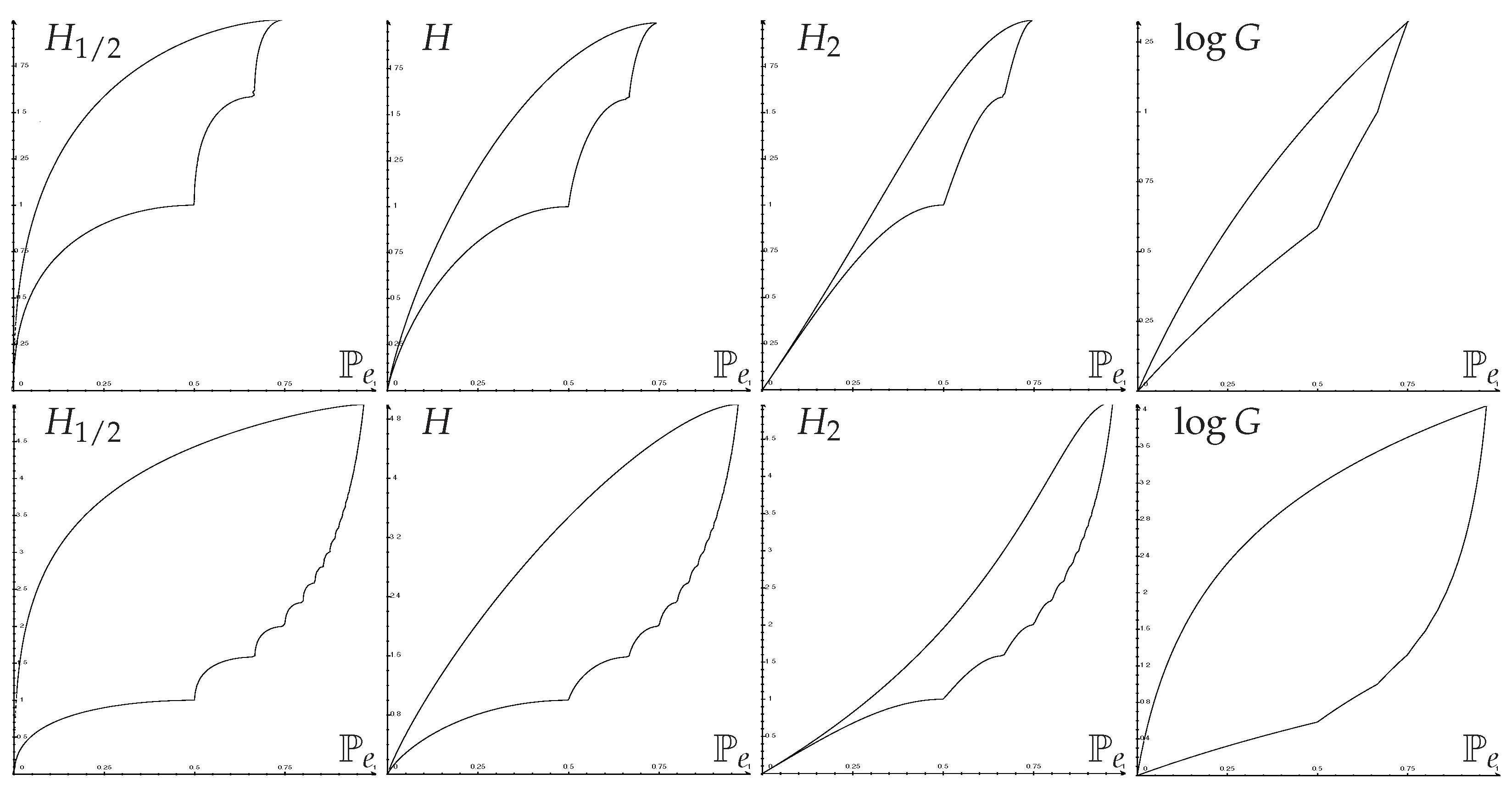
Applying s-concavity of entropies or to (51) gives closed-form upper bounds of entropies as a function of , known as Fano inequalities; and closed-form lower bounds, known as reverse Fano inequalities. Figure 1 shows some optimal regions.
The original Fano inequality was an upper bound on conditional entropy as a function of . It can be shown that upper bounds in the conditional case are unchanged. Lower bounds of conditional entropies or -entropies, however, have to be slightly changed due to the average operation inside the function F (see Section 3 above) by taking the convex enveloppe (piecewise linear) of the lower curve on . In this way, one recovers easily the results of [20] for H,11] for , and [14,17] for G and .
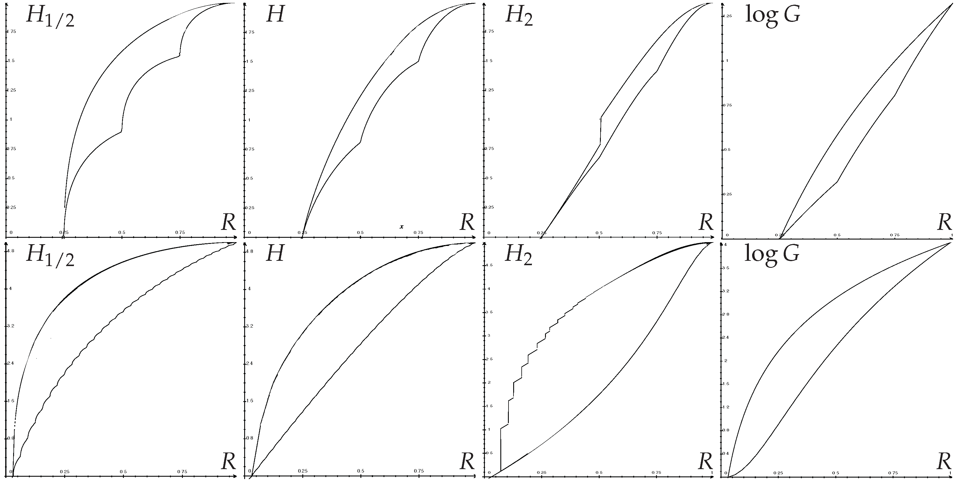
Likewise, applying s-concavity of entropies or to (52) gives closed-form upper bounds of entropies as a function of R, similar to Pinsker inequalities; and closed-form lower bounds, similar to reverse Pinsker inequalities. Figure 2 shows some optimal regions.
The various Pinsker and reverse Pinsker inequalities that can be found in the literature give bounds between and for general q. Such inequalities find application in Quantum physics [21] and to derive lower bounds on the minimax risk in nonparametric estimation [22]. As they are of more general applicability, they turn out not to be optimal here since we have optimized the bounds in the particular case . Using our method, one again recovers easily previous results of [23] (and [24], Theorem 26) for H, and improves previous inequalities used for several applications [3,4,6].
6. Conclusions
Using a simple method based on “mixing” or majorization, we have established optimal (Fano-type and Pinsker-type) bounds between entropic quantities (, ) and statistical quantities (, R) in an interplay between information theory and statistics. As a perspective, similar methodology could be developed for statistical distance to an arbitrary (not necessarily uniform) distribution.
Funding
This research received no external funding.
Institutional Review Board Statement
Not applicable.
Informed Consent Statement
Not applicable.
Data Availability Statement
Not applicable.
Conflicts of Interest
The author declares no conflict of interest.
References
- Maurer, U.M. A Universal Statistical Test for Random Bit Generators. J. Cryptol. 1992, 5, 89–105. [Google Scholar] [CrossRef]
- Pliam, J.O. Guesswork and Variation Distance as Measures of Cipher Security. In SAC 1999: Selected Areas in Cryptography, Proceedings of the International Workshop on Selected Areas in Cryptography, Kingston, ON, Canada, 9–10 August 1999; Heys, H., Adams, C., Eds.; Lecture Notes in Computer Science; Springer: Berlin/Heidelberg, Germany, 1999; Volume 1758, pp. 62–77. [Google Scholar]
- Chevalier, C.; Fouque, P.A.; Pointcheval, D.; Zimmer, S. Optimal Randomness Extraction from a Diffie-Hellman Element. In Advances in Cryptology—EUROCRYPT 2009, Proceedings of the Annual International Conference on the Theory and Applications of Cryptographic Techniques, Cologne, Germany, 26–30 April 2009; Joux, A., Ed.; Lecture Notes in Computer Science; Springer: Berlin/Heidelberg, Germany, 2009; Volume 5479, pp. 572–589. [Google Scholar]
- Shoup, V. A Computational Introduction to Number Theory and Algebra, 2nd ed.; Cambridge University Press: Cambridge, UK, 2009. [Google Scholar]
- Schaub, A.; Boutros, J.J.; Rioul, O. Entropy Estimation of Physically Unclonable Functions via Chow Parameters. In Proceedings of the 57th Annual Allerton Conference on Communication, Control, and Computing, Monticello, IL, USA, 24–27 September 2019. [Google Scholar]
- Killmann, W.; Schindler, W. A Proposal for Functionality Classes for Random Number Generators. Ver. 2.0, Anwendungshinweise und Interpretationen zum Schema (AIS) 31 of the Bundesamt für Sicherheit in der Informationstechnik. 2011. Available online: https://www.bsi.bund.de/SharedDocs/Downloads/EN/BSI/Certification/Interpretations/AIS_31_Functionality_classes_for_random_number_generators_e.pdf?__blob=publicationFile&v=4 (accessed on 11 March 2021).
- Fehr, S.; Berens, S. On the conditional Rényi entropy. IEEE Trans. Inf. Theory 2014, 60, 6801–6810. [Google Scholar] [CrossRef]
- Arimoto, S. Information measures and capacity of order α for discrete memoryless channels. In Topics in Information Theory; Csiszár, I., Elias, P., Eds.; Colloquium Mathematica Societatis János Bolyai, 2nd ed.; North Holland: Amsterdam, The Netherlands, 1977; Volume 16, pp. 41–52. [Google Scholar]
- Liu, Y.; Cheng, W.; Guilley, S.; Rioul, O. On conditional alpha-information and its application in side-channel analysis. In Proceedings of the 2021 IEEE Information Theory Workshop (ITW2021), Online, 17–21 October 2021. [Google Scholar]
- Rioul, O. Variations on a theme by Massey. IEEE Trans. Inf. Theory 2022, 68, 2813–2828. [Google Scholar] [CrossRef]
- Sason, I.; Verdú, S. Arimoto–Rényi Conditional Entropy and Bayesian M-Ary Hypothesis Testing. IEEE Trans. Inf. Theory 2018, 64, 4–25. [Google Scholar] [CrossRef]
- Massey, J.L. Guessing and entropy. In Proceedings of the IEEE International Symposium on Information Theory, Trondheim, Norway, 27 June–1 July 1994; p. 204. [Google Scholar]
- Arikan, E. An inequality on guessing and its application to sequential decoding. IEEE Trans. Inf. Theory 1996, 42, 99–105. [Google Scholar] [CrossRef] [Green Version]
- Sason, I.; Verdú, S. Improved Bounds on Lossless Source Coding and Guessing Moments via Rényi Measures. IEEE Trans. Inf. Theory 2018, 64, 4323–4346. [Google Scholar] [CrossRef] [Green Version]
- Cover, T.M.; Thomas, J.A. Elements of Information Theory, 2nd ed.; John Wiley & Sons: Hoboken, NJ, USA, 2006. [Google Scholar]
- van Erven, T.; Harremoës, P. Rényi divergence and Kullback-Leibler divergence. IEEE Trans. Inf. Theory 2014, 60, 3797–3820. [Google Scholar] [CrossRef] [Green Version]
- Béguinot, J.; Cheng, W.; Guilley, S.; Rioul, O. Be my guess: Guessing entropy vs. success rate for evaluating side-channel attacks of secure chips. In Proceedings of the 25th Euromicro Conference on Digital System Design (DSD 2022), Maspalomas, Gran Canaria, Spain, 31 August–2 September 2022. [Google Scholar]
- Rioul, O. A primer on alpha-information theory with application to leakage in secrecy systems. In Geometric Science of Information, Proceedings of the 5th Conference on Geometric Science of Information (GSI’21), Paris, France, 21–23 July 2021; Lecture Notes in Computer Science; Springer: Berlin/Heidelberg, Germany, 2021; Volume 12829, pp. 459–467. [Google Scholar]
- Marshall, A.W.; Olkin, I.; Arnold, B.C. Inequalities: Theory of Majorization and Its Applications, 2nd ed.; Springer Series in Statistics; Springer: Berlin/Heidelberg, Germany, 2011. [Google Scholar]
- Ho, S.W.; Verdú, S. On the Interplay Between Conditional Entropy and Error Probability. IEEE Trans. Inf. Theory 2010, 56, 5930–5942. [Google Scholar] [CrossRef]
- Audenaert, K.M.R.; Eisert, J. Continuity Bounds on the Quantum Relative Entropy—II. J. Math. Phys. 2011, 52, 7. [Google Scholar] [CrossRef] [Green Version]
- Tsybakov, A.B. Introduction to Nonparametric Estimation; Springer Series in Statistics; Springer: Berlin/Heidelberg, Germany, 2009. [Google Scholar]
- Ho, S.W.; Yeung, R.W. The Interplay Between Entropy and Variational Distance. IEEE Trans. Inf. Theory 2010, 56, 5906–5929. [Google Scholar] [CrossRef]
- Sason, I.; Verdú, S. f-Divergence Inequalities. IEEE Trans. Inf. Theory 2016, 62, 5973–6006. [Google Scholar] [CrossRef]
Figure 1.
Optimal regions: Entropies (in bits) vs. error probability. Top row ; bottom row .

Figure 2.
Optimal regions: Entropies (in bits) vs. randomness R. Top row ; bottom row .

Publisher’s Note: MDPI stays neutral with regard to jurisdictional claims in published maps and institutional affiliations. |
© 2022 by the author. Licensee MDPI, Basel, Switzerland. This article is an open access article distributed under the terms and conditions of the Creative Commons Attribution (CC BY) license (https://creativecommons.org/licenses/by/4.0/).
Share and Cite
MDPI and ACS Style
Rioul, O. What Is Randomness? The Interplay between Alpha Entropies, Total Variation and Guessing. Phys. Sci. Forum 2022, 5, 30. https://doi.org/10.3390/psf2022005030
AMA Style
Rioul O. What Is Randomness? The Interplay between Alpha Entropies, Total Variation and Guessing. Physical Sciences Forum. 2022; 5(1):30. https://doi.org/10.3390/psf2022005030
Chicago/Turabian StyleRioul, Olivier. 2022. "What Is Randomness? The Interplay between Alpha Entropies, Total Variation and Guessing" Physical Sciences Forum 5, no. 1: 30. https://doi.org/10.3390/psf2022005030