Dynamic Modeling and Control of a Coupled Reforming/Combustor System for the Production of H₂ via Hydrocarbon-Based Fuels

Abstract

The present work aims to provide insights into the dynamic operation of a coupled reformer/combustion unit that can utilize a variety of saturated hydrocarbons (HCs) with 1–4 C atoms towards H₂ production (along with CO₂). Within this concept, a preselected HC-based feedstock enters a steam reforming reactor for the production of H₂ via a series of catalytic reactions, whereas a sequential postprocessing unit (water gas shift reactor) is then utilized to increase H₂ purity and minimize CO. The core unit of the overall system is the combustor that is coupled with the reformer reactor and continuously provides heat (a) for sustaining the prevailing endothermic reforming reactions and (b) for the process feed streams. The dynamic model as it is initially developed, consists of ordinary differential equations that capture the main physicochemical phenomena taking place at each subsystem (energy and mass balances) and is compared against available thermodynamic data (temperature and concentration). Further on, a distributed control scheme based on PID (Proportional–Integral–Derivative) controllers (each one tuned via Ziegler–Nichols/Z-N methodology) is applied and a set of case studies is formulated. The aim of the control scheme is to maintain the selected process-controlled variables within their predefined set-points, despite the emergence of sudden disturbances. It was revealed that the accurately tuned controllers lead to (a) a quick start-up operation, (b) minimum overshoot (especially regarding the sensitive reactor temperature), (c) zero offset from the desired operating set-points, and (d) quick settling during disturbance emergence.

1. Introduction

It is widely known that greenhouse gas emissions are directly related to the exaggeration of Global Warming. Specifically, CO₂ emissions are an inevitable harmful source that mainly derive from conventional power plants (coal and lignite based), cement production, steel industries, and petrochemical plants [1,2,3,4]. As these “heavy industrial units” are still relying on fossil fuels, serious issues of feedstock depletion need to be tackled by today’s academic and research society. A common way to alleviate these dual energy and environmental concerns is to evaluate the use of alternative fuels that can be based (directly or indirectly) on renewable energy sources (RES) or unexploited hydrocarbon-based sources [5].

H₂ as an efficient energy carrier, is considered to be a clean energy source since its combustion is accompanied by zero emissions (only pure water is produced). H₂-based applications range from simple domestic and stationary implementations (e.g., heating, energy production) up to transportation utilities (e.g., hybrid vehicles) [6,7]. Nevertheless, the lack of a reliable distribution network and a safety management handling requires H₂ to be produced from suitable feedstock. The latter can comprise either water electrolysis or hydrocarbons steam reforming [8,9].

Based on the currently available technologies, steam reforming of hydrocarbons is a mature and widely applied process for the production of H₂. Numerous studies exist in literature and each one delves into a specific area of analysis. Experimental studies that deal with C1–C2 [10,11,12], C3–C4 [9,13], and higher hydrocarbons [14,15,16,17] have already postulated that modeling studies are necessary in order to properly comprehend the system dynamics that involve the interaction of several subsystems. As these subsystems operate continuously and sequentially, such modeling studies can serve as the basis for an advanced control and scaled-up design that will ensure an economically feasible H₂ production.

Since the highlight of this study is the process modeling and control of a hydrocarbon-based reformer unit, the focus will be based on similar studies (unless mentioned otherwise). Zečević and Bolf [18] presented a methodology for the continuous monitoring and subsequent optimization of a natural gas steam reformer. In their study, they highlighted the need for an external combustor unit, whereas their proposed topology revealed the need for a distributed control system. Stamps and Gatzke [19] developed dynamic models for a series of connected subsystems dealing with methanol steam reforming. Similarly, their proposed control system was based on distributed feedback controllers (PI type). Xiang et al. [20] screened alternative process flow diagrams in order to ensure a flexible heat integration for the ethanol steam reforming. As was derived, the increased heat demands of steam reforming are crucial and should be taken into account during process modeling and control studies. A linearized dynamic model that was devoted to the mapping of manipulated and controlled variables was presented by El-Sharkh et al. [21], whereas a similar attempt was provided by Pravin et al. [22]. These groups highlighted the complexity of interconnections between subsystems and discussed how a well-implemented control system can lead to an efficient system operation. Lin et al. [23] developed a detailed dynamic model for a methane reformer system that was utilized in two different plant-wide control schemes. Such an approach was considered as a prerequisite for the rejection of emerged disturbances (e.g., catalyst deactivation). On the same road Funke et al. [24] focused on modeling heat transfer phenomena that can significantly suppress the catalytic reformer operation. A multivariable approach (modeling and control) was presented by Pukrushpan et al. [25] and accurately focused on the operation of a PEM fuel cell, whereas Biset et al. [26] presented a control-based study in HYSYS software for an ethanol reforming unit. In one of the most concrete studies, Hu et al. [27] developed linear models for a diesel-based reforming unit and focused mainly on the reformer operation. As presented, the conventional feedback and feed-forward strategies did not lead to an efficient operation and, thus, an advanced control scheme had to be proposed instead. While not based on a modelling study, Schäde et al. [28] screened the reforming of saturated HCs towards H₂ production in a concept that truly highlighted the need for flexible steam reformers that can handle a variety of feedstock. Meanwhile, it was shown that each HC-based fuel required different heat demands that should also be taken into account during process modelling and control.

While, the process modeling and control of hydrocarbon-based reformer systems has been applied in literature, it still receives increasing scientific attention. Most studies focus on the individual subsystem operation (mainly the reformer that operates with a single component feedstock), whereas the integrated operation that consists of heat integration units (such as a combustion unit that can effectively allow the heat coupling of process streams) has not been assessed dynamically in detail. Along with the aforementioned literature shortcomings, this study evaluates as hydrocarbon-based fuel a mixture of low quality propane that can be found in (bio)refineries (e.g., effluent cracked gases from pyrolysis units that include C1–C4 hydrocarbons or streams that refer to low quality propane). To this end, the main focus of this study is (a) to develop compact dynamic models for simulating the integrated operation of a coupled reformer/combustion unit followed by a sequential H₂ postprocessing stage (Water Gas Shift reactor WGS) and (b) to apply distributed PID controllers for ensuring a stable and realistic operation and within predefined desired set-points. The structure of this paper is as follows: Section 2 describes the H₂ production system including the main mathematical modeling set. Then, Section 3 analyzes the applied control scheme and the required mapping of manipulated-controlled variables, whereas Section 4 summarizes the theoretical framework by a typical simulation study based on certain operating scenarios.

2. Mathematical Modeling and Process System Description

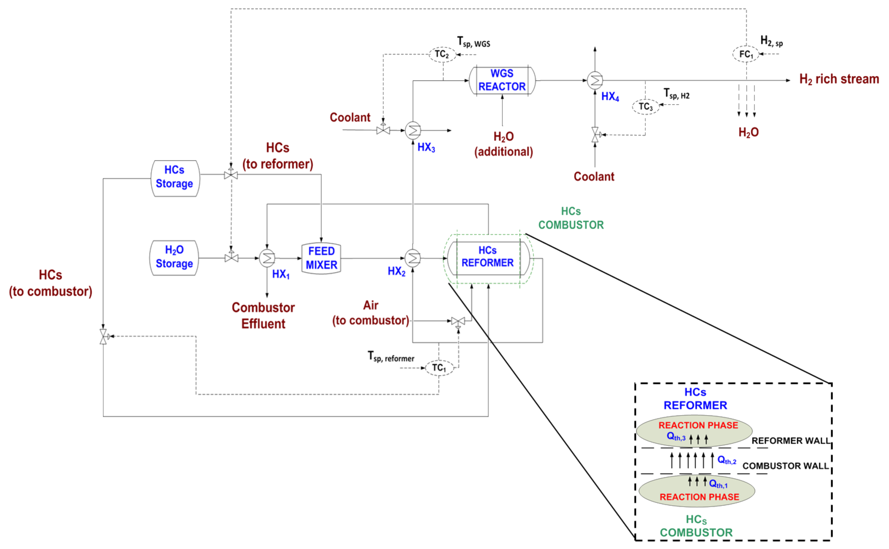
2.1. Process System Description

Figure 1 presents the autonomous H₂ production system that was developed for this study and is accompanied by

Table 1. Reactions taking place at the coupled reforming/combustor system.

Reactions	Reaction Kinetics
HCs Reformer Unit   R1a/b: CnH2n+2 + n∙H2O→ n∙CO + (2n + 1)∙H2 R2: CO + H2O ↔ H2 + CO2 R3: CO + 3∙H2 →CH4 + H2O	$\begin{array}{l}{R}_{1a/b}=k_{1,0}\cdot \exp (-\frac{E_{1a/b}}{R\cdot T})\cdot C_{C_n{H}_{2n+2}}\cdot {(C_{H_{2}O})}^n\\ R_2=k_{2,0}\cdot \exp (-\frac{E_2}{R\cdot T})\cdot (C_{CO}\cdot C_{H_{2}O}-\frac{C_{C{O}_2}\cdot C_{H_2}}{K_{eq,1}}),K_{eq,1}=\exp (\frac{E_{eq,1}}{R\cdot T}{-\mathrm{C}}_{eq,1})\\ R_3=k_{3,0}\cdot \exp (-\frac{E_3}{R\cdot T})\cdot (C_{CO}\cdot {(C_{H_2})}^3-\frac{C_{C{H}_4}{C}_{H_{2}O}}{K_{eq,2}}),K_{eq,2}=\exp (\frac{E_{eq,2}}{R\cdot T}{-\mathrm{C}}_{eq,2})\end{array}$
WGS Unit CO + H2O ↔ H2 + CO2	$R_4=k_{4,0}\cdot \exp (-\frac{E_4}{R\cdot T})\cdot C_{CO}\cdot C_{H_{2}O}$
Combustor Unit   CnH2n+2 + (3n + 1)/2∙O2 → n∙CO2 + (n + 1)∙H2O	$R_5=k_{5,0}\cdot \exp (-\frac{E_5}{R\cdot T})\cdot C_{C_n{H}_{2n+2}}\cdot C_{O_2}$

(reactions taking place at each subsystem). The aim of this study is to focus on the reforming of a mixture of hydrocarbons that are more rarely studied in literature. However, the overall process is presented generically in order to highlight the flexibility of the system to handle hydrocarbons with 1–4 C atoms (in the case of oxygenated HCs such as methanol, ethanol, etc., slight modifications are required). To this end, the saturated HCs shown in Table 1 refer to a mixture of propane and butane (C₃H₈, C₄H₁₀), as this is a realistic case with a low quality propane feedstock in refineries. Alternatively, this rich in saturated HC mixture could simulate effluent cracked gases from pyrolysis units that may also include C1–C4 hydrocarbons [29]. Reaction (power law) kinetics are referring to simplified forms of Arrhenius type.

Hydrocarbons and water are initially mixed prior to entering the steam reforming reactor. This process operation requires the preheating of water at a temperature of 120–140 °C and then, the further heating of the steam/HC mixture at the reformer operating temperature (650–850 °C). This two stage heat exchanging takes place in HX1 through the combustor hot effluent and in HX2 through the reformer hot outlet, respectively. This heat coupling has already proved that process economics and system efficiency can be significantly improved [30,31] when an autonomous operation is required (e.g., stand-alone applications). The steam/HC mixture enters the catalytic steam reformer where a set of reactions take place as shown in Table 1 along with the respective kinetics (reaction enthalpies are estimated as a function of temperature/pressure.). A fundamental improvement with this H₂ production process and as compared to other literature studies, is the coupling of the reformer with a combustion unit (combustor) in order to utilize available heat for sustaining the endothermic reactions. The combustor utilizes the exact same hydrocarbon and the wall-to-wall connection ensures the continuous heat provision through combustion reactions (Table 1). As shown in Figure 1, there are three main heat transferring zones: (a) from the combustion reaction phase to the combustor wall as Q_th,1, (b) from the combustor wall to the reformer wall as Q_th,2, and (c) from the reformer wall to the reformer reaction phase as Q_th,3. The reformer exit stream includes H₂, CO, CO₂, and unconverted HC and is cooled in two stages (a) in HX2 as a part of heat coupling with the inlet reformer stream (mentioned previously) and (b) in HX3 at the required WGS reactor operating temperature (280–400 °C). The WGS reactor is necessary in order to minimize CO by-product (through water gas shift reaction) that can be detrimental in H₂-fed units such as PEM fuel cells, hydrogenation reactors, or even H₂ storage [32]. The exit of the WGS reactor is cooled down in order to condense and remove H₂O, and then the high purity H₂/CO₂ stream can be further utilized. Rich H₂/CO₂ streams have recently revealed their significance in CO₂ hydrogenation reactions towards fuels [33,34,35,36] and for this reason the proposed operating scheme leads to this H₂/CO₂ production

2.2. Dynamic Modeling

As was briefly discussed in the introduction, several types of mathematical models are available in literature describing solely the operation of catalytic reactors, heat exchangers, combustion units, and other auxiliary units. The dual objective of this section is not to provide detailed and complex models for the various subsystems, but to provide a suitable and well-recognized dynamic model set that can (a) capture the main operating features and (b) provide the basis for control-oriented simulation studies. Only in this way the proposed mathematical model would be accompanied by an easy-to-handle computational implementation. The mathematical formulation consisting of the ordinary differential equations (nonlinear) was solved via Runge–Kutta method in Matlab Software. Supplementary assumptions and related modeling equations are shown collectively in the Appendix as well.

2.2.1. HCs Combustion Unit

The system combustion unit utilizes hydrocarbon (as the main combustion fuel) for the necessary heat production. The generated heat is transferred through the combustor wall to the reformer in order to sustain the endothermic reactions (Figure 1). Clearly, this unit is crucial for the efficient operation of the integrated system, since an ineffective or deficient heat provision would lead to a problematic H₂ production or even serious start-up issues. To this end, this unit is modeled as a CSTR reactor and includes energy and mass balances along with necessary algebraic equations. Regarding the energy balance, two ordinary differential equations simulate the dynamics of the effluent gas stream temperature (T_out,c) and the combustor wall temperature (T_wall,c). The latter indirectly refers to the heat that is provided to the reformer reactor (see Section 2.2.2).

$$\frac{d({\rho }_{out,c}c{p}_{out,c}{V}_{out,c}{T}_{out,c})}{dt}=(c{p}_{in,c}{\rho }_{in,c}{Q}_{in,c}{T}_{in,c}-c{p}_{out,c}{\rho }_{out,c}{Q}_{out,c}{T}_{out,c})\pm {\displaystyle \sum Q_{th}{}_{,total,combustor}}$$

(1)

$$m_{c}c{p}_c\frac{d{T}_{wall,c}}{dt}=(Q_{th,1}-Q_{th,2})$$

(2)

$$Q_{th,total,,combustor}=Q_{chem,c}-Q_{rad,c}-Q_{th,1}$$

(3)

where ρ_out,c and ρ_in,c are the outlet and inlet fluid density at the combustor in kg/m³, cp_out,c and cp_in,c the outlet and inlet fluid heat capacity at the combustor in J/K·kg, V_out,c the fluid volume in m³, T_out,c and T_in,c the outlet and inlet fluid temperature at the combustor in K, Q_out,c and Q_in,c the outlet and inlet fluid flowrate at the combustor in m³/s, Q_{th,total,combustor} the total combustor heat in W, Q_chem,c the heat that is generated from combustion reactions in W (Table 1), Q_rad,c the heat that is radiated to the environment in W, Q_th,1 the heat that is transferred from the bulk of the combustor to its wall in W, Q_th,2 the heat that is transferred from the combustor wall to the reformer wall in W, m_c the combustor mass in kg, cp_c the combustor material, and T_wall,c the combustor wall temperature in K. In the Appendix, the detailed expressions of the heat duties are provided for the HCs combustion unit.

As far as the mass balances are of concern, the following equations are utilized for each one of the involved components i (Table 1) in order to simulate their concentration dynamics:

$$\frac{d(C_i{}_{,out,c}{V}_{out,c})}{dt}=C_{i,in,c}{Q}_{in,c}-C_{i,out,c}{Q}_{out,c}\pm {\displaystyle \sum {\nu }_{i,j}{R}_j}$$

(4)

where i refers to the nine involved components (C_nH_2n+2:CH₄, C₃H₈, C₄H₁₀) O₂, N₂, CO, CO₂, H₂O, H₂), C_i,out,c, and C_i,in,c the outlet and inlet concentration of component i in mol/m³, ν_i,j is the stoichiometric coefficient of component i in reaction j (Table 1).

2.2.2. HCs Reformer Reactor

The reformer utilizes the preheated HCs/steam mixture towards H₂ production (Table 1). Following the same principles as with the combustor unit, this reactor is also modeled as a CSTR reactor and includes energy and mass balances along with necessary algebraic equations. Regarding energy balance, two ordinary differential equations simulate the dynamics of the reformer exit stream temperature (T_out,reformer) and the reformer wall temperature T_{wall,reformer}). The latter indirectly refers to the heat that is provided to the reformer reactor from the combustor (see Section 2.2.1 and Figure 1).

$$\begin{array}{l}\frac{d({\rho }_{out,reformer}c{p}_{out,reformer}{V}_{out,reformer}{T}_{out,reformer})}{dt}=\\ (c{p}_{in,reformer}{\rho }_{in,reformer}{Q}_{in,reformer}{T}_{in,reformer}-c{p}_{out,reformer}{\rho }_{out,reformer}{Q}_{out,reformer}{T}_{out,reformer})\pm {\displaystyle \sum Q_{th}{}_{,total,reformer}}\end{array}$$

(5)

$$m_{ref}c{p}_{ref}\frac{d{T}_{wall,reformer}}{dt}=(Q_{th,2}-Q_{th,3})$$

(6)

$$Q_{th,total,reformer}=Q_{chem,reformer}-Q_{rad,reformer}+Q_{th,3}$$

(7)

As far as mass balances are of concern the following equations are utilized for each one of the involved components i (Table 1):

$$\frac{d(C_i{}_{,out,reformer}{V}_{out,reformer})}{dt}=C_{i,in,reformer}{Q}_{in,reformer}-C_{i,out,reformer}{Q}_{out,reformer}\pm {\displaystyle \sum {\nu }_{i,j}{R}_j}$$

(8)

All variables and parameters have already been denoted in Section 2.2.1 for the combustor and are similarly used here under the subscript reformer. At the Appendix , the detailed expressions of the heat duties are provided for the HCs reformer reactor.

2.2.3. Heat Exchangers HX1–HX4

In all four heat exchangers (HX) there is a heat transfer from a hot stream to a cold stream (or vice versa). Specifically, (a) in HX1 the combustor effluent provides heat for steam generation prior to feed mixing, (b) in HX2 the reformer exit stream provides heat to the reformer inlet stream, (c) in HX3 and HX4 the WGS reactor inlet and outlet are cooled down, respectively, via the use of a coolant. Mass balances are not required for HXs, since there is no material transformation (a slight change only takes place for the fluid density as shown in Appendix A equations). Hence, two energy balances are developed and simulate the interchange of heat between the hot and cold streams.

$$\begin{array}{l}\frac{d({\rho }_{out,H{X}_{1-4},hot}c{p}_{out,H{X}_{1-4}hot}{V}_{out,H{X}_{1-4},hot}{T}_{out,H{X}_{1-4},hot})}{dt}=\\ (c{p}_{in,H{X}_{1-4},hot}{\rho }_{in,H{X}_{1-4},hot}{Q}_{in,H{X}_{1-4},hot}{T}_{in,H{X}_{1-4},hot}-c{p}_{out,H{X}_{1-4},hot}{\rho }_{out,H{X}_{1-4},hot}{Q}_{out,H{X}_{1-4},hot}{T}_{out,H{X}_{1-4},hot})\pm {\displaystyle \sum Q_{th}{}_{,total,H{X}_{1-4}}}\end{array}$$

(9)

$$\begin{array}{l}\frac{d({\rho }_{out,H{X}_{1-4},cold}c{p}_{out,H{X}_{1-4},cold}{V}_{out,H{X}_{1-4},cold}{T}_{out,H{X}_{1-4},cold})}{dt}=\\ (c{p}_{in,H{X}_{1-4},cold}{\rho }_{in,H{X}_{1-4},cold}{Q}_{in,H{X}_{1-4},cold}{T}_{in,H{X}_{1-4},cold}-c{p}_{out,H{X}_{1-4},cold}{\rho }_{out,H{X}_{1-4},cold}{Q}_{out,H{X}_{1-4}cold}{T}_{out,H{X}_{1-4},cold})\mp {\displaystyle \sum Q_{th}{}_{,total,H{X}_{1-4}}}\end{array}$$

(10)

$$Q_{th,total,H{X}_{1-4}}=U{A}_{HX1-4}(T_{out,H{X}_{1-4},hot}-T_{out,H{X}_{1-4},cold})$$

(11)

All variables and parameters have already been denoted in Section 2.2.1 and Section 2.2.2 for the combustor and reformer units (and also in the Nomenclature), and are similarly used here under the subscript of HX_1-4 for cold and hot streams.

2.2.4. Water Gas Shift (WGS) Reactor

The WGS reactor utilizes the reformer exit along with additional water (if needed) for the necessary minimization of CO through water gas shift reaction (Table 1). Following the same principles as with the combustor and reformer units, this reactor is also modelled as a CSTR reactor and includes energy and mass balances along with necessary algebraic equations. Regarding the energy balance, a single ordinary differential equation simulates the dynamics of the WGS exit stream temperature (T_out,WGS). Contrary to the combustor and the reformer, the WGS reactor does not require external heating or cooling for this proposed concept.

$$\begin{array}{l}\frac{d({\rho }_{out,WGS}c{p}_{out,WGS}{V}_{out,WGS}{T}_{out,WGS})}{dt}=\\ (c{p}_{in,WGS}{\rho }_{in,WGS}{Q}_{in,WGS}{T}_{in,WGS}-c{p}_{out,WGS}{\rho }_{out,WGS}{Q}_{out,WGS}{T}_{out,WGS})\pm {\displaystyle \sum Q_{th}{}_{,total,WGS}}\end{array}$$

(12)

As far as mass balances are of concern the following equations are utilized for each one of the involved components i (Table 1):

$$\frac{d(C_i{}_{,out,WGS}{V}_{out,WGS})}{dt}=C_{i,in,WGS}{Q}_{in,WGS}-C_{i,out,WGS}{Q}_{out,WGS}\pm {\displaystyle \sum {\nu }_{i,j}{R}_j}$$

(13)

All variables and parameters have already been denoted in Section 2.2.1 and 2.2.2for the combustor and reformer units, and are similarly used here under the subscript of WGS. In the Appendix, the detailed expressions of the heat duties are provided for the WGS reactor.

2.2.5. Model Comparison with Available Data (Steady-State Simulation)

As has already been postulated, the process system that was developed is too difficult to be validated against experimental data, since there are not enough process systems (to the best of the authors’ knowledge) that follow the proposed unit integration and with the respective feedstock flexibility. In order to ensure that simulation results will be as realistic as possible, Figure 1 was simulated both with Aspen Plus and with the developed dynamic model (under the same inlet and operating conditions). The results are shown in the

Table 2. Comparison of Aspen Plus and process modeling results (at steady state conditions).

Process Variable	Aspen Plus Results	Dynamic Modeling Results
Reformer Exit	H2: 71–74%	H2: 72.5–74%
	CO2: 11.5–12.5%	CO2: 12.0–13%
	CO: 13.5–14.5%	CO: 14.2–15%
	CH4: 1.0–1.2%	CH4: 1.0–1.1%
WGS Exit	H2: 74–76.5%	H2: 75.5–77%
	CO2: 22–23%	CO2: 22.3–23%
	CO: 1.2–1.4%	CO: 1.0–1.5%
	CH4: 0.9–1.1%	CH4: 0.9–1%

Reformer Operating Conditions: HCs inlet flowrate: 6.5–9 mol/h, H₂O inlet flowrate: 18–24 mol/h, T = 700 °C, P = 1.28 atm. Combustor Operating Conditions: T = 800 °C, P = 1.28 atm. WGS Operating Conditions: HCs inlet flowrate: 3.6–4.2 mol/h, Air Excess 20%, T = 280 °C, P = 1.28 atm.

that follows.

As can be seen, both modelling pathways lead to similar results with minor deviations. Hence, the developed mathematical model is considered realistic enough in order to be used in subsequent control studies. An important point to notice from the above table is the fact that the final process exit stream comprises H₂/CO₂ at a ratio of ≈3 which is the feedstock requirement of CO₂ hydrogenation units towards fuel production [33,34,35,36].

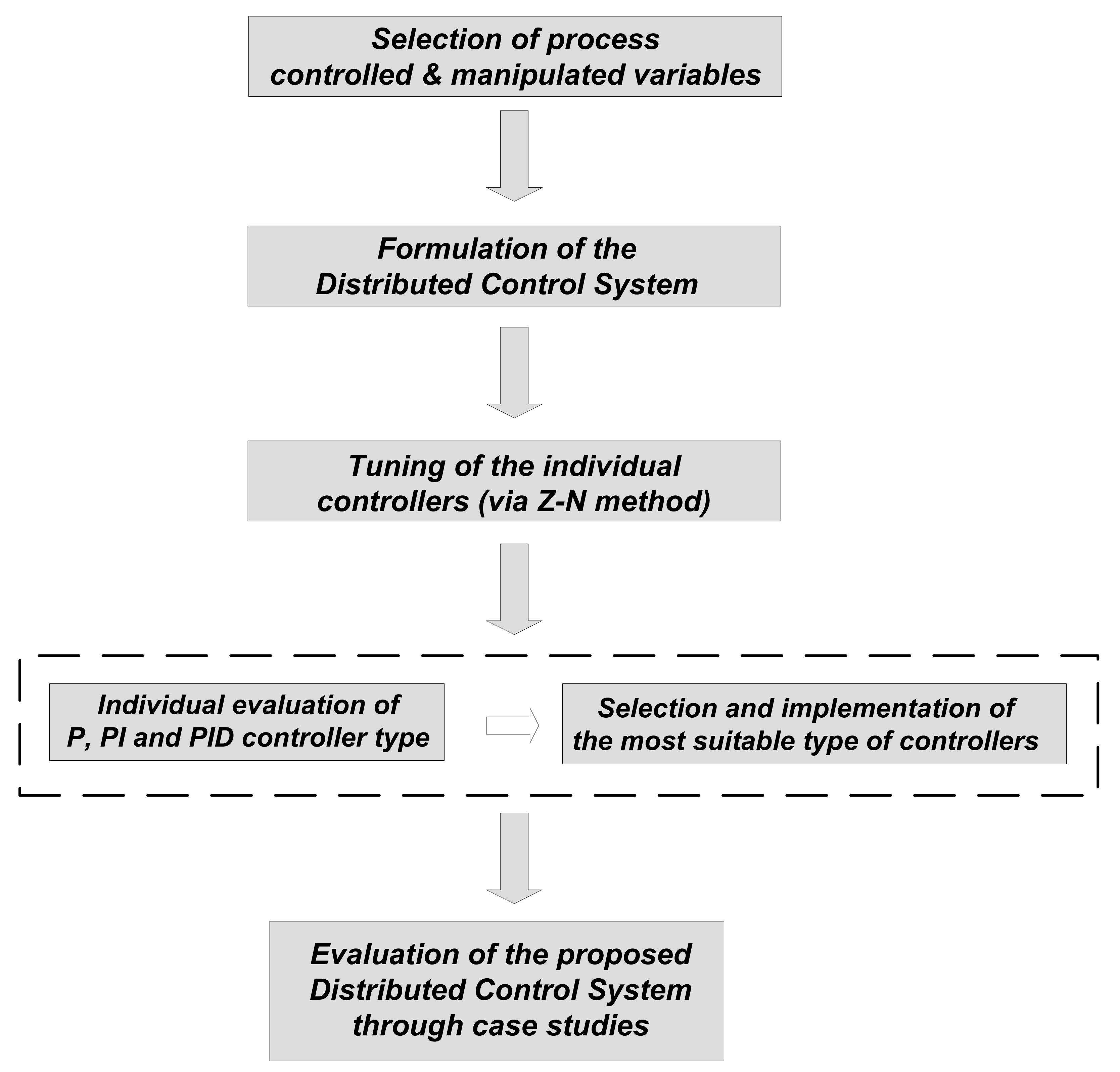
3. Control Structure Implementation

In order to apply and evaluate the proposed distributed control system, the following steps are implemented (Figure 2) and discussed in detail afterwards:

• Step 1: Selection of process controlled and manipulated variables (based on predefined targets and not through a systematic approach for this preliminary study) and formulation of the Distributed Control System (placement of feedback controllers in the studied process).
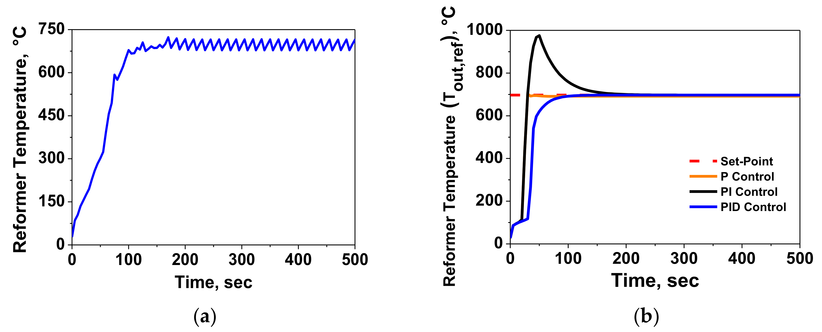
• Step 2: Tuning of the applied controllers and individual evaluation of the different types (P, PI, PID).
• Step 3: Implementation of the selected (based on Step 2) type of controllers (either, P, PI, or PID) and fine tuning (if necessary).
• Step 4: Simulation of case scenarios based on realistic operation modes.

Step 1: As shown in Figure 1, four controllers are distributed to the proposed system: (i) TC1 that controls the reformer exit temperature (equivalently the operating temperature inside the reactor) by manipulating the HCs feed rate at the combustor, (ii) TC2 that controls the WGS inlet temperature by manipulating the coolant flowrate at HX3, (iii) TC3 that controls the WGS exit temperature by manipulating the coolant flowrate at HX4, and (iv) FC1 that controls the H₂ production rate by manipulating the HCs feed rate at the reformer. It is highlighted that the temperature of the steam reformer inlet is not required to be controlled independently, due to the fact that it stems indirectly from the control actions taking place in TC1 and FC1. This compact heat coupling in HX1, HX2 has been initially designed and assessed offline via Aspen Plus so that the reformer inlet temperature will always be within an acceptable range (±20 °C from the reformer operating temperature) as long as TC1 and FC1 controllers are tuned and operate properly. In this way, the steam reformer catalytic operation can be protected from off-range specifications. The applied control scheme while not assessed nor selected systematically, crucially provides a safe operation for the main system units (two reactors and the coupled combustor).

Step 2: The next step is the tuning of the applied controllers via the empirical and widely known method of Ziegler–Nichols. This method is quite simple in its implementation (individually at each controller) since all controllers operate as proportional ones (P-control) until each controlled variable shows oscillation of a constant magnitude. The critical gain and the critical period of oscillation (K_cr, P_cr) is recorded and used for the evaluation of the three P-I-D controller parameters according to known correlations [37]. As a typical example of tuning, TC1 controller performance is shown in Figure 3a under constant oscillations (exactly similar results were obtained during the tuning of the other controllers as well). The critical gain and the critical period of oscillation is recorded at 0.005 and 70 s respectively, and based on these values the suitable K, T_i, T_d controller parameters are estimated for each candidate P, PI, or PID controller, respectively (see

Table 3. Selection of controllers based on the tuning strategy.

Controller	Type of Controller	K	Ti	Td
TC1	PID	2.27 × 10−6	150.0 s	7.0 s
TC2	PID	5.89 × 10−3	130.0 s	10.0 s
TC3	PID	2.94 × 10−3	150.0 s	13.75 s
FC1	PID	4.00 × 10−2	100.0 s	4.3 s

).

Step 3: Each of the three controller types (P, PI, or PID) is implemented and the dynamic response of the reformer operating temperature is quantitatively and qualitatively assessed as a representative example. As shown in Figure 3b, the proportional (P) controller leads to an aggressive response that maintains a low but still, significant error (≈7–10 °C). On the other hand, the PI controller while it eliminates the error it creates a detrimental overshoot of more than 200 °C (totally damaging for the reforming catalyst). Finally, the PID controller satisfactorily eliminates the error and maintains a smooth dynamic start-up that is suggested in such sensitive reactor units. Based on this strategy, Table 3 shows the best selection of the controllers TC1–TC3 and FC1 for the studied system.

$$\mathrm{PID}\mathrm{Controller}:p(t)=p_s+K_{}\cdot [\epsilon (t)+\frac{1}{T_i}{\displaystyle \int \epsilon (t)dt}+T_d\cdot \frac{d\epsilon (t)}{dt}]$$

(14)

$$\mathrm{Error}\mathrm{at}\mathrm{the}\mathrm{Controller}:\epsilon (t)=Y_{sp}(t)-Y(t)$$

(15)

where p(t) is the output signal of the controller, p_s the controller bias (assumed zero) at ε(t = 0) = 0, K is the controller gain, T_i is the controller integral time constant, T_d is the controller derivative time constant, ε(t) is the input signal (error) to the controller, Y_sp the controlled variable set point, and Y the controlled variable (e.g., temperature at TC1–TC3, flowrate at FC1).

Step 4: Simulations of case scenarios based on realistic operation modes are presented and analyzed in detail in Section 4.

4. Evaluation of Control Structure: Analysis and Results of Simulated Scenarios

In order to evaluate the performance of the distributed control system, two realistic operating scenarios are formulated. In the 1st scenario, the overall control system targets specific set-point trajectories (either constant or transient), whereas in the 2nd scenario the control system targets the rejection of an emerged disturbance.

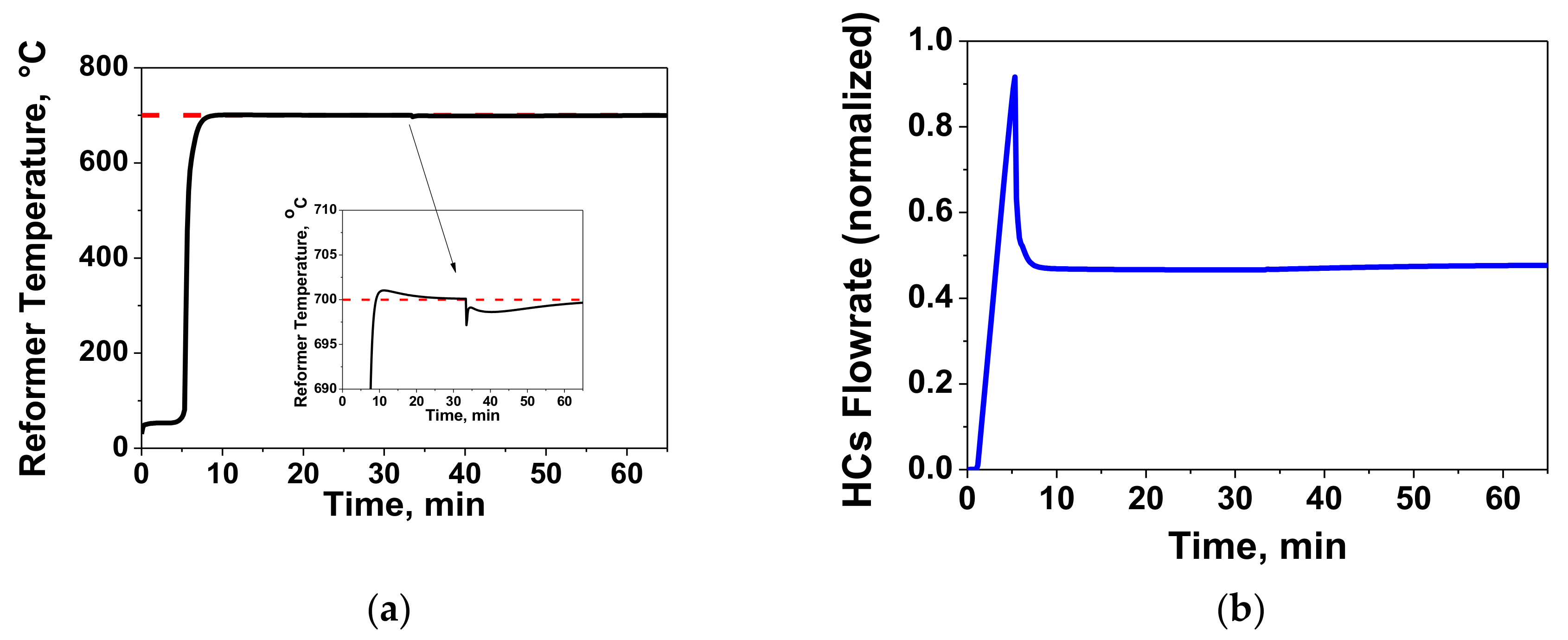
4.1. Set-Point Trajectory (Scenario 1)

In Scenario 1, the applied controllers are meant to regulate the respective controlled variables within their predefined set-point trajectories. A transient state is applied on the H₂ production rate (+20% increase) at the exit of the WGS reactor at t = 33 min. Figure 4 shows the dynamic performance of the TC1 controller. Specifically, the operating reformer temperature reaches the set-point value of 700 °C at around t = 10 min (Figure 4a), which is considered an acceptable time period during start-up operation. After reaching this targeted value, an insignificant overshoot is observed, as a result of the excellent PID controller tuning. During the transient response at the H₂ production rate controller (will be discussed later), a ≈5 °C decrease is initially observed, but quickly tackled by the controller. The reason for this small temperature reduction is attributed to the fact that the need for a higher H₂ production rate at the exit of the integrated system enables a higher HCs flowrate at the inlet of the reformer. Simultaneously, this increase in the HCs flowrate initiates higher heat consumption (at the respective reactions presented in Table 1) and thus, reformer temperature is slightly decreased. However, TC1 controller maintains the temperature level by slightly increasing the HCs flowrate at the inlet of the combustor (Figure 4b), which provides more heat to the steam reforming reactor.

Next, the TC2 and TC3 controller performance is evaluated in Figure 5 and Figure 6, respectively. As can be seen in Figure 5a, the inlet stream temperature at the WGS reactor is maintained excellently within the predefined set-point and without any overshoot during its operation. During the transient response at t = 33 min, Figure 5b records an expected increase on the coolant flowrate due to the fact that the heat content at the inlet of HX3 is now increased (higher reformer effluent due to the need to provide higher H₂ at the exit of the system). However, the dynamic response at HX3 does not allow the exit temperature to vary significantly at t = 33 min.

Following the same principles in our analysis, Figure 6 shows that the exit stream temperature at the WGS reactor (HX4) is maintained excellently, within the predefined set-point and with a 2–3 °C overshoot during its operation. Similarly to Figure 5b, Figure 6b records an increase in the coolant flowrate due to the fact that the heat content at the inlet of HX4 is increased. It is highlighted that the coolant flowrates at both TC2 and TC3 initiate only when needed (not at t = 0 s but only when a higher from the set-point temperature was recorded).

Finally, Figure 7 shows the performance of the FC1 controller at the exit of the WGS reactor. Specifically, Figure 7a shows the dynamic response of H₂ production rate at the exit of the WGS that is maintained excellently before and after the transient change (t = 33 min). As can be seen, the FC1 controller operates smoothly as it captures quickly this transient modification by quickly manipulating the HCs flowrate at the reformer inlet (Figure 7b).

4.2. Disturbance Rejection (Scenario 2)

In Scenario 2, the applied controllers are required to maintain the process-controlled variables within their predefined set-point trajectories when a sudden disturbance arises. In order to provide a realistic operating scenario, the catalyst performance deteriorates suddenly at t = 33 min. Such a change means that lower H₂ will be produced (worst case scenario). As can be seen in Figure 8a and during the disturbance emergence, the reformer operating temperature is increased as a consequence of the catalyst deactivation (suppression of the endothermic reactions). Nonetheless, TC1 controller quickly tackles this deviation, reduces the HCs flowrate at the combustor (Figure 8b), and restores the reformer temperature at its predefined set point. After the disturbance emergence, the system operation fully recovers after 4–5 min.

Next, the TC2 and TC3 controller performance is evaluated (Figure 9 and Figure 10, respectively). As can be seen in Figure 9a, the inlet stream temperature at the WGS reactor is maintained excellently within the predefined set-point and without any variation during the disturbance emergence. On the other hand, Figure 9b shows that at t = 33 min a higher coolant flowrate is required. This dynamic response was expected, since Figure 8a revealed that the disturbance emergence (catalyst malfunction) induces higher reformer exit temperature and thus, higher coolant requirements (≈10%).

Similarly, Figure 10a shows that the exit stream temperature at the WGS reactor is maintained excellently within the predefined set-point, whereas Figure 10b records a slight decrease at the coolant flowrate requirements that quickly ensure the maintenance of WGS exit.

Finally, Figure 11 shows the performance of the FC1 controller at the exit of the WGS reactor. As was expected, the decrease of catalyst activity at the reformer induces lower H₂ production (Figure 11a at t = 33 min) and hence, the FC1 controller induces a higher HCs flowrate at the reformer (Figure 11b) in order to suppress this disturbance. Figure 11a shows the dynamic response of H₂ flowrate at the exit of the WGS that is maintained acceptably.

5. Discussion

The present study developed a dynamic model and a distributed control scheme for a coupled reformer/combustor H₂ production system. The core objective was the capturing of the dynamic operation of the integrated process as a single entity. The mathematical model was developed with an insight to capture the main physicochemical properties and the inherent dynamics of the involved subsystems. Overall, the applied control scheme quantitatively and qualitatively revealed that the temperature controller TC1 maintained accurately the reformer operating temperature within the predefined set-point both at the transient response Scenario 1 and at the disturbance rejection Scenario 2. Τhe emergence of catalyst malfunction induced only a slight overshoot of ≈10 °C which was tackled quickly, effectively manipulating the HCs flowrate at the combustor. Meanwhile, the dynamic transient change at t = 33 min did not induce significant modifications since the reformer temperature only slightly deviated as a result of the excellent TC1 controller response. For the other two temperature controllers (TC2 and TC3), it was shown that neither the disturbance nor the transient modification created any significant changes at the WGS inlet at outlet temperature since the respective controllers maintained their set-point levels accurately. Finally, according to the results of this study, the flow controller FC1 regulated effectively the H₂ production rate. Even though a critical disturbance emerged, the FC1 controller quickly manipulated the HCs flowrate at the reformer in order to restore the production rate within the specified set-point (Scenario 2). Furthermore, this controller quickly responded towards a higher production rate when needed (Scenario 1 with the transient modification).

Such a simplified yet compact study can be considered as the basis of ensuring the development of advanced process control schemes that can be readily applied in similar reforming pilot plants. Due to the need to maintain a “green process”, a crucial highlight has to be made: since the HCs feedstock is meant to refer to refinery cracked gases (C1–C4) or to low quality C3–C4 stream, then the produced H₂/CO₂ stream should be further postprocessed towards fuels production [33,34,35,36]. Furthermore, the formulation of this study and the overall modeling methodology could be utilized in advanced process design and control studies that will simultaneously manage the design of the control structure along with potential modification in the operating scheme (e.g., further heat recycling, splitting streams).

References

1. Chen, T.D.; Kockelman, K.M. Carsharing’s life-cycle impacts on energy use and greenhouse gas emissions. Transp. Res. Part D Transp. Environ. 2016, 47, 276–284. [Google Scholar] [CrossRef]
2. Liu, W.; King, D.; Liu, J.; Johnson, B.; Wang, Y.; Yang, Z. Critical material and process issues for CO2 separation from coal-powered plants. JOM 2009, 61, 36–44. [Google Scholar] [CrossRef]
3. Manzolini, G.; Giuffrida, A.; Cobden, P.D.; van Dijk, H.A.J.; Consonni, F. Techno-economic assessment of SEWGS technology when applied to integrated steel-plant for CO2 emission mitigation. Int. J. Greenh. Gas Control 2020, 94, 102935. [Google Scholar] [CrossRef]
4. Proaño, L.; Sarmiento, A.T.; Figueredo, M.; Cobo, M. Techno-economic evaluation of indirect carbonation for CO2 emissions capture in cement industry: A system dynamics approach. J. Clean. Prod. 2020, 263, 121457. [Google Scholar] [CrossRef]
5. Marocco, P.; Ferrero, D.; Gandiglio, M.; Ortiz, M.M.; Santarelli, M. A study of the techno-economic feasibility of H2-based energy storage systems in remote areas. Energ. Convers. Manag. 2020, 211, 112768. [Google Scholar] [CrossRef]
6. Veziroglu, A.; MacArio, R. Fuel cell vehicles: State of the art with economic and environmental concerns. Int. J. Hydrogen. Energy 2011, 36, 25–43. [Google Scholar] [CrossRef]
7. Kim, J.; Kim, T. Compact PEM fuel cell system combined with all-in-one hydrogen generator using chemical hydride as a hydrogen source. Appl. Energy 2014, 160, 945–953. [Google Scholar] [CrossRef]
8. Meloni, E.; Martino, M.; Palma, V. A Short Review on Ni Based Catalysts and Related Engineering Issues for Methane Steam Reforming. Catalysts 2020, 10, 352. [Google Scholar] [CrossRef] [Green Version]
9. Do, J.Y.; Chava, R.K.; Son, N.; Kim, J.; Park, N.-K.; Lee, D.; Seo, M.W.; Ryu, H.-J.; Chi, J.H.; Kang, M. Effect of Ce Doping of a Co/Al2O3 Catalyst on Hydrogen Production via Propane Steam Reforming. Catalysts 2018, 8, 413. [Google Scholar] [CrossRef] [Green Version]
10. Pashchenko, D. Combined methane reforming with a mixture of methane combustion products and steam over a Ni-based catalyst: An experimental and thermodynamic study. Energy 2019, 185, 573–584. [Google Scholar] [CrossRef]
11. Gao, N.; Cheng, M.; Quan, C.; Zheng, Y. Syngas production via combined dry and steam reforming of methane over Ni-Ce/ZSM-5 catalyst. Fuel 2020, 2731, 117702. [Google Scholar] [CrossRef]
12. Keshavarz, A.R.; Soleimani, M. Nano-sized Ni/(CaO)x-(Al2O3)y catalysts for steam pre-reforming of ethane and propane in natural gas: The role of CaO/Al2O3 ratio to enhance conversion efficiency and resistance to coke formation. J. Nat. Gas Sci. Eng. 2017, 45, 1–10. [Google Scholar] [CrossRef]
13. Recupero, V.; Pino, L.; Vita, A.; Cipitı, F.; Cordaro, M.; Laganà, M. Development of a LPG fuel processor for PEFC systems: Laboratory scale evaluation of autothermal reforming and preferential oxidation subunits. Int. J. Hydrogen. Energy 2005, 30, 963–971. [Google Scholar] [CrossRef]
14. Sasaki, K.; Takahashi, I.; Kuramoto, K.; Tomomichi, K.; Terai, T. Reactions on Ni-YSZ cermet anode of solid oxide fuel cells during internal steam reforming of n-octane. Electrochim. Acta 2018, 2591, 94–99. [Google Scholar] [CrossRef]
15. Park, N.-K.; Lee, Y.J.; Kwon, B.C.; Lee, T.J.; Kang, S.H.; Hong, B.U.; Kim, T. Optimization of Nickel-Based Catalyst Composition and Reaction Conditions for the Prevention of Carbon Deposition in Toluene Reforming. Energies 2019, 12, 1307. [Google Scholar] [CrossRef] [Green Version]
16. Al-Musa, A.; Al-Saleh, M.; Ioakeimidis, Z.C.; Ouzounidou, M.; Yentekakis, I.V.; Konsolakis, M.; Marnellos, G.E. Hydrogen production by iso-octane steam reforming over Cu catalysts supported on rare earth oxides (REOs). Int. J. Hydrogen. Energy 2014, 39, 1350–1363. [Google Scholar] [CrossRef]
17. Al-Musa, A.A.; Ioakeimidis, Z.S.; Al-Saleh, M.S.; Al-Zahrany, A.; Marnellos, G.E.; Konsolakis, M. Steam reforming of iso-octane toward hydrogen production over mono- and bi-metallic CueCo/CeO2 catalysts: Structure-activity correlations. Int. J. Hydrogen. Energy 2014, 39, 19541–19554. [Google Scholar] [CrossRef]
18. Zečević, N.; Bolf, N. Integrated Method of Monitoring and Optimization of Steam Methane Reformer Process. Processes 2020, 8, 408. [Google Scholar] [CrossRef] [Green Version]
19. Stamps, A.T.; Gatzke, E.P. Dynamic modeling of a methanol reformer—PEMFC stack system for analysis and design. J. Power Sources 2006, 161, 356–370. [Google Scholar] [CrossRef]
20. Xiang, D.; Li, P.; Yuan, X. Process Modeling, Optimization, and Heat Integration of Ethanol Reforming Process for Syngas Production with High H2/CO Ratio. Processes 2019, 7, 960. [Google Scholar] [CrossRef] [Green Version]
21. El-Sharkh, M.Y.; Rahman, A.; Alam, M.S.; Byrne, P.C.; Sakla, A.A.; Thomas, T. A dynamic model for a stand-alone PEM fuel cell power plant for residential applications. J. Power Sources 2004, 138, 199–204. [Google Scholar] [CrossRef]
22. Pravin, P.S.; Gudi, R.D.; Bhartiya, S. Dynamic Modeling and Control of an Integrated Reformer-Membrane-Fuel Cell System. Processes 2018, 6, 169. [Google Scholar]
23. Lin, S.T.; Chen, Y.H.; Yu, C.C.; Liu, Y.C.; Lee, C.H. Dynamic modeling and control structure design of an experimental fuel processor. Int. J. Hydrogen. Energy 2006, 31, 413–426. [Google Scholar] [CrossRef]
24. Funke, M.; Kühl, H.D.; Faulhaber, S.; Pawlik, J. A dynamic model of the fuel processor for a residential PEM fuel cell energy system. Chem. Eng. Sci. 2009, 64, 1860–1867. [Google Scholar] [CrossRef]
25. Pukrushpan, J.T.; Stefanopoulou, A.G.; Peng, H. Control of Fuel Cell Power Systems, 1st ed.; Springer: London, UK, 2005. [Google Scholar]
26. Biset, S.; Deglioumini, L.N.; Basualdo, M.; Garcia, V.M.; Serra, M. Analysis of the control structures for an integrated ethanol processor for proton exchange membrane fuel cell systems. J. Power Sources 2009, 192, 107–113. [Google Scholar] [CrossRef] [Green Version]
27. Hu, Y.; Chmielewski, D.J.; Papadias, D. Autothermal reforming of gasoline for fuel cell applications: Controller design and analysis. J. Power Sources 2008, 182, 298–306. [Google Scholar] [CrossRef]
28. Schädel, B.T.; Duisberg, M.; Deutschmann, O. Steam reforming of methane, ethane, propane, butane, and natural gas over a rhodium-based catalyst. Catal. Today 2009, 142, 42–51. [Google Scholar] [CrossRef]
29. Chen, B.; Yang, T.; Xiao, W.; Nizamani, A.K. Conceptual Design of Pyrolytic Oil Upgrading Process Enhanced by Membrane-Integrated Hydrogen Production System. Processes 2019, 7, 284. [Google Scholar] [CrossRef] [Green Version]
30. Ipsakis, D.; Ouzounidou, M.; Papadopoulou, S.; Seferlis, P.; Voutetakis, S. Dynamic modeling and control analysis of a methanol autothermal reforming and PEM fuel cell power system. Appl. Energy 2017, 208, 703–718. [Google Scholar] [CrossRef]
31. Delikonstantis, E.; Scapinello, M.; Stefanidis, G.D. Investigating the Plasma-Assisted and Thermal Catalytic Dry Methane Reforming for Syngas Production: Process Design, Simulation and Evaluation. Energies 2017, 10, 1429. [Google Scholar] [CrossRef] [Green Version]
32. Sarma, P.J.; Gardner, C.L.; Chugh, S.; Sharma, A.; Kjeang, E. Strategic implementation of pulsed oxidation for mitigation of CO poisoning in polymer electrolyte fuel cells. J. Power Sources 2020, 468, 228352. [Google Scholar] [CrossRef]
33. Konsolakis, M.; Lykaki, M.; Stefa, S.; Carabineiro, S.A.C.; Varvoutis, G.; Papista, E.; Marnellos, G.E. CO2 Hydrogenation over Nanoceria-Supported Transition Metal Catalysts: Role of Ceria Morphology (Nanorods versus Nanocubes) and Active Phase Nature (Co versus Cu). Nanomaterials 2019, 9, 1739. [Google Scholar] [CrossRef] [PubMed] [Green Version]
34. Konsolakis, M.; Lykaki, M. Recent Advances on the Rational Design of Non-Precious Metal Oxide Catalysts Exemplified by CuOx/CeO2 Binary System: Implications of Size, Shape and Electronic Effects on Intrinsic Reactivity and Metal-Support Interactions. Catalysts 2020, 10, 160. [Google Scholar] [CrossRef] [Green Version]
35. Varvoutis, G.; Lykaki, M.; Stefa, S.; Papista, E.; Carabineiro, S.A.C.; Marnellos, E.; Konsolakis, M. Remarkable efficiency of Ni supported on hydrothermally synthesized CeO2 nanorods for low-temperature CO2 hydrogenation to methane. Catal. Commun. 2020, 142. in press. [Google Scholar] [CrossRef]
36. Díez-Ramírez, J.; Sánchez, P.; Kyriakou, V.; Zafeiratos, S.; Marnellos, G.E.; Konsolakis, M.; Dorado, F. Effect of support nature on the cobalt-catalyzed CO2 hydrogenation. J. CO2 Util. 2017, 21, 562–571. [Google Scholar] [CrossRef]
37. Astrom, K.J.; Hagglund, T. PID Controllers: Theory, Design, and Tuning, 2nd ed.; Instrument Society of America: Research Triangle Park, NC, USA, 1995. [Google Scholar]
Figure 1. Coupled reforming/combustor system for H2 production along with a distributed control system.
Processes 08 01243 g001
Figure 2. Implementation of the proposed control structure and related algorithm.
Processes 08 01243 g002
Figure 3. (a) Temperature profile of the reformer during TC1 controller tuning with Z-N method and (b) temperature profile of the reformer under three types of TC1 tuned controllers (P, PI, and PID).
Processes 08 01243 g003
Figure 4. (a) Temperature profile of the reformer (TC1 controller) and (b) HCs flowrate manipulation at the combustor.
Processes 08 01243 g004
Figure 5. (a) Temperature profile of the WGS inlet (TC2 controller) and (b) coolant flowrate manipulation at the HX3.
Processes 08 01243 g005
Figure 6. (a) Temperature profile of the WGS exit (TC3 controller) and (b) coolant flowrate manipulation at the HX4.
Processes 08 01243 g006
Figure 7. (a) H2 production rate (FC1 controller) and (b) HCs flowrate manipulation at the reformer.
Processes 08 01243 g007
Figure 8. (a) Temperature profile of the reformer (TC1 controller) and (b) HCs flowrate manipulation at the combustor.
Processes 08 01243 g008
Figure 9. (a) Temperature profile of the WGS inlet (TC2 controller) and (b) coolant flowrate manipulation at the HX3.
Processes 08 01243 g009
Figure 10. (a) Temperature profile of the WGS exit (TC3 controller) and (b) coolant flowrate manipulation at the HX4.
Processes 08 01243 g010
Figure 11. (a) H2 production profile at WGS exit (FC1 controller) and (b) HCs flowrate manipulation at the reformer.
Processes 08 01243 g011