Combining Mechanistic Modeling and Raman Spectroscopy for Monitoring Antibody Chromatographic Purification

Abstract

Chromatography is widely used in biotherapeutics manufacturing, and the corresponding underlying mechanisms are well understood. To enable process control and automation, spectroscopic techniques are very convenient as on-line sensors, but their application is often limited by their sensitivity. In this work, we investigate the implementation of Raman spectroscopy to monitor monoclonal antibody (mAb) breakthrough (BT) curves in chromatographic operations with a low titer harvest. A state estimation procedure is developed by combining information coming from a lumped kinetic model (LKM) and a Raman analyzer in the frame of an extended Kalman filter approach (EKF). A comparison with suitable experimental data shows that this approach allows for the obtainment of reliable estimates of antibody concentrations with reduced noise and increased robustness.

1. Introduction

The application of spectroscopic techniques to monitor chromatographic processes in the frame of the so-called process analytical technology (PAT) initiative is very promising due to its potential for gathering important on-line process information in a non-invasive way [1,2,3,4,5]. Available spectroscopic techniques range from UV/vis and Fourier transform infrared spectroscopy to dynamic light scattering [6]. Several applications of Raman spectroscopy have been reported in upstream processing [7,8,9], showing the potential of this technology, which often requires specific modeling techniques, such as partial least squares (PLS) regression, to extract the desired information from the measured spectra. Recently, a successful implementation of Raman spectroscopy for the on-line monitoring of monoclonal antibody (mAb) concentrations in downstream processing was reported by Feidl et al [10]. An ad hoc developed flow cell enabled the integration of the Raman technology into the capture (protein A) step of a mAb manufacturing process, providing accurate on-line estimates of mAb concentration. However, in spite of these results, the use of this technology remains limited due to the intrinsic weakness of the Raman signal [11,12,13].

In this work, we explore the possibility of overcoming these difficulties by combining estimates from the Raman signal with the predictions of a mechanistic model. This is particularly convenient in the chromatographic purification of mAbs because these processes are well understood and reliable mechanistic simulation models are available [14]. It has been already shown in many other areas that the combination of deterministic knowledge and on-line measurements can lead to more accurate and reliable estimates [15,16,17,18], e.g., by using extended Kalman filtering (EKF) [19]. While a general introduction to Kalman filtering is given in [20], a more detailed description is provided in [21].

In this work, the implementation of an EKF for a chromatographic capture step to estimate antibody concentration is shown by combining the information of a deterministic chromatographic model with on-line information derived from Raman-based PLS estimates. In particular, the objective is to monitor the chromatographic breakthrough curves of a low-concentrated monoclonal antibody harvest. The beneficial effect of the combination of the two approaches with respect to the stand-alone Raman and chromatographic model is discussed.

2. Materials and Methods

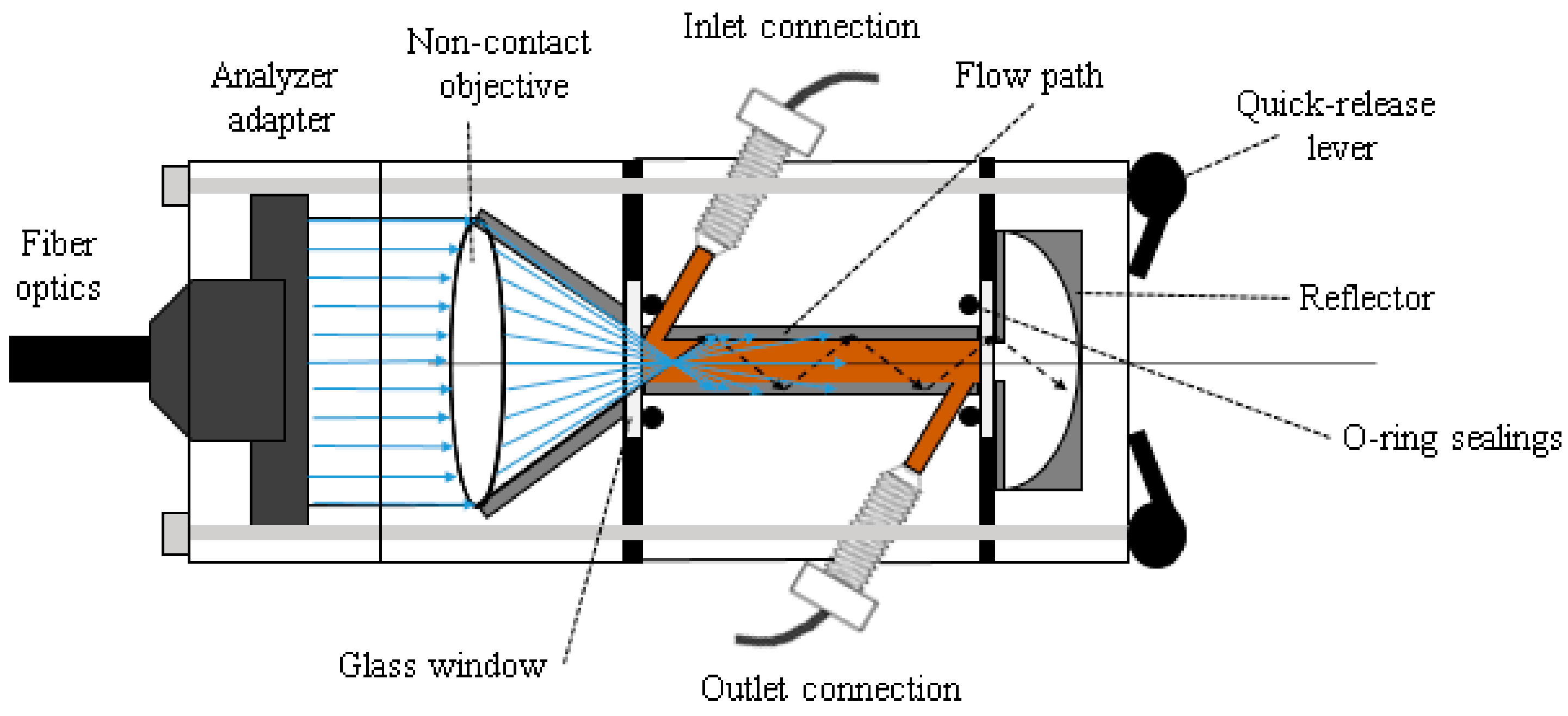
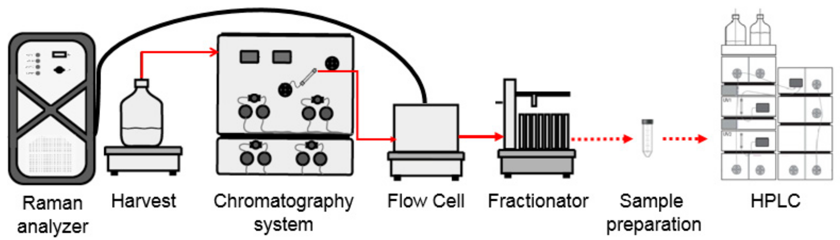
2.1. Raman Spectral Acquisition and Flow Cell

Raman spectra were acquired with a Kaiser RamanRxn2 analyzer (Kaiser Optical Systems, Inc., Ann Arbor, MI, USA), including a 785 nm laser at 400 mW and a cooled charged-coupled device (CCD) detector, measuring inelastic photon scattering across a 150–3425 cm⁻¹ wavenumber range. A laser exposure time of 30 s was chosen to collect the single scan spectra. A flow cell with an optimized flow characteristic, signal enhancement, pressure tolerance, and a single use potential was developed. A schematic illustration of the flow cell is shown in Figure 1. It includes four main modules: (A) An analyzer adapter, which connects the flow cell to the Raman analyzer via a fiber cable; (B) a non-contact objective to focus the laser beam within the flow path; (C) a flow path, which guides the sample longitudinally to the laser beam; and (D) a reflector, reflecting scattered and unscattered light to the analyzer via the flow path. In the application to chromatographic purifications, the inlet connection is coupled to the elution stream, and the outlet connection is linked to the sample fractionator.

2.2. Cell Culture Supernatant

Two cell culture supernatant pools containing a recombinant mAb with product concentrations between 0.30 and 0.60 mg/mL were obtained from a CHO cell perfusion process, as reported in [22]. Besides cell filtering through the perfusion hollow fiber module (0.5 µm pore size, Spectrum Laboratories, Netherlands), no other treatment was applied to the supernatant, which therefore contained a large quantity of impurities, e.g., media components, host cell proteins (HCP, 3 × 10⁵ ppm), DNA (4 × 10⁴ ppm) and high molecular weight (HMW) species (1.1%).

2.3. Breakthrough Runs and Reference Analytic

Fifteen breakthrough (BT) runs were performed on MabSelect SuRe columns (GE Healthcare, Uppsala, Sweden), prepacked by Repligen GmbH (Ravensburg, Germany, 0.5 × 5 cm), as described in [10]. The feed concentration, flow rate, and the fraction duration were changed between the different BT runs, as described in

Table 1. Chromatographic settings and Raman measurements availability of performed breakthrough curves.

	Breakthrough Curve ID	Feed Conc. (mg/mL)	Feed Flow Rate (mL/Min)	Run Duration (Min)	Fraction Duration (Min)	Raman Measurements
Used for PLS and EKF	BT#1	0.34	1.0	200	8	+
	BT#2	0.34	1.5	230	4	+
	BT#3	0.34	1.0	250	6	+
	BT#4	0.42	1.5	130	2	+
	BT#5	0.42	1.0	120	3.5	+
	BT#6	0.42	1.0	170	3.5	+
Used for LKM fitting	BT#7	0.43	1.0	240	4	-
	BT#8	0.43	1.5	160	4	-
	BT#9	0.43	0.5	480	4	-
	BT#10	0.30	0.5	690	10	-
	BT#11	0.30	1.5	230	10	-
	BT#12	0.30	1.0	340	10	-
	BT#13	0.60	0.5	200	3	-
	BT#14	0.60	1.5	80	3.5	-
	BT#15	0.60	1.0	120	3.5	-

. Since several Raman measurements were acquired while collecting the sample of a single fraction (between 4 and 16 spectra per fraction), a spline approach was applied to interpolate missing reference measurements for each Raman spectrum.

The mAb concentrations were determined off-line by HPLC with an analytical standard deviation of 0.01 mg/mL as described in [23]. The HMW, HCP, and DNA content of the harvest were determined as described in [10]. A schematic illustration of the experimental set-up is shown in Figure 2.

2.4. Chemometric Modeling Procedure

All calculations were performed with MATLAB R2018a (Mathworks, Natick, MA, USA) using in-house developed routines, if not stated otherwise. The modeling procedure included Savitzky–Golay smoothing with a second polynomial order and a frame size of 51 Raman shift wavenumbers [24], spectrum wise standard normal variate (SNV) processing [25], and Raman shift wavenumber wise mean centering on spectra and reference values [26]. The removal of spectral regions based on the bioprocess modeling experience resulted in spectral ranges of 450–1820 cm⁻¹, 1880–2530 cm⁻¹ and 2590–3100 cm⁻¹ to eliminate interferences with the window material and water as well as non-informative regions. No derivative, Raman shift wavenumber selection, or automated outlier removal tools were applied. The nonlinear iterative partial least squares (NIPALS) algorithm [27] was used to calibrate predictive PLS models, which regressed spectral data on HPLC reference values, including a threefold cross validation (CV) [28]. The optimal number of latent variables (LV) was determined based on the minimum CV error.

After calibrating the model on five different BT runs, the model was tested on an external BT run, i.e., not included in the calibration. In order to evaluate the model performance, the root mean square error was calculated for both cross validation (RMSECV) and external prediction (RMSEP), using Equation (1), where ${\widehat{y}}_i$ is the predicted value of the i-th observation, $y_i$ is the corresponding measured value, and n is the total number of observations:

$$RMSE=\sqrt{\frac{1}{n}{{\displaystyle \sum }}_{i=1}^n{\left(y_i-{\widehat{y}}_i\right)}^2}$$

(1)

Furthermore, the coefficient of determination ($R^2$) was calculated for the external prediction as follows:

$$R^2=1-\frac{{{\displaystyle \sum }}_{i=1}^n{\left(y_i-{\widehat{y}}_i\right)}^2}{{{\displaystyle \sum }}_{i=1}^n{\left(y_i-\overline{y}\right)}^2}$$

(2)

A rotational approach was used to judge upon the model transferability and data set similarity. Hence, sets were rotated in order to have every BT run in the external prediction set once, as shown in

Table 2. Modeling procedure including the Raman-PLS (partial least squares) calibration, mechanistic model fitting, as well as the tuning, validation and perturbation of the extended Kalman filtering (EKF).

For a given Rot i

1. Raman-PLS calibration:

$PL{S}_{Rot i}$ ← calibrate Raman-PLS on BT#1–6 except BT#i

2. Mechanistic model fitting:

LKM ← fit LKM on BT#7–15 with respective process inputs ($P{I}_{BT\#7-15}$)

3. EKF tuning:

$EK{F}_{Rot i}$ ← tune EKF (Q, R, $k_Q^{Rot i}$) on BT#1–6 except BT#i

for n = BT#1–6 except BT#i

$k_{Q_{best}}^n=mi{n}_{k_Q}RMSE{P}_{EK{F}_n}$

end for

$k_Q^{Rot i}=$ average $k_{Q_{best}}^n$ for all n

4. EKF validation:

Run $EK{F}_{Rot i}$ with inputs $LKM$, $P{I}_{Rot i}, PL{S}_{Rot i} \mathrm{and} k_Q^{Rot i}$

5. EKF perturbation:

for n = 1–200 simulations

$P{I}_{RS}$ = random sampling of $\epsilon$, $c_{in},$ $Q_{flow}$ from Gaussian probability distribution

Run $EK{F}_{Rot i}$ with inputs $LKM$,$P{I}_{RS}, PL{S}_{Rot i} \mathrm{and} k_Q^{Rot i}$

end for

. As an example, to build the model for rotation 1 (ROT1), the data of BT#2–6 were used for model calibration and tested on BT#1 (for further details, see [10]).

2.5. Deterministic Modeling Procedure

The chromatographic process was modelled using the lumped kinetic model (LKM) [14,29]:

$$\frac{\partial c}{\partial t}=-v\frac{\partial c}{\partial x}+D_L\frac{{\partial }^{2}c}{\partial x^2}-\phi \frac{\partial q}{\partial t} t\in \left[0,t_{end}\right], x\in \left[0,L_{Col}\right]$$

(3)

$$\frac{\partial q}{\partial t}=k_m\left(q^{*}-q\right)$$

(4)

where $c$ is the liquid phase concentration of the protein, $t$ is the time, $t_{end}$ is the end of the BT run, $v$ is the interstitial velocity ($v=\frac{Q_{flow}}{A_{col} \epsilon }$), $Q_{flow}$ is the volumetric flow rate (see Table 1), $A_{col}$ is the column cross sectional area ($A_{col}$= 0.196 cm²), $\epsilon$ is the bed porosity ($\epsilon$= 0.36 [30]), $x$ is the coordinate along the column longitudinal axis, $L_{Col}$ is the column length ($L_{Col}$= 5 cm), $D_L$ is the apparent axial dispersion coefficient, $\phi =\left(1-\epsilon \right)/\epsilon$ is the phase ratio of the column, $q$ is the solid phase concentration of the protein, $k_m$ is the mass transfer coefficient, and $q^{*}$ is the equilibrium solid phase concentration of the protein.

The following initial conditions were applied:

$$c\left(t=0,x\right)=c_0\left(x\right)$$

(5)

$$q\left(t=0,x\right)=q_0\left(x\right)$$

(6)

They were then combined with the classical Danckwerts’ boundary conditions:

$$c\left(t>0,x=0\right)=c_{in}\left(t\right)+\frac{D_L}{v}{\left.\frac{\partial c}{\partial x}\right]}_{x=0}$$

(7)

$${\left.\frac{\partial c}{\partial x}\right]}_{x=L_{col}}=0$$

(8)

where $c_{in}\left(t\right)$ is the feed concentration (see Table 1). Both $c_0\left(x\right)$ and $q_0\left(x\right)$ are zero for all values of $x$. The apparent axial dispersion coefficient $D_L$ can be estimated from the reduced van Deemter equation [31]:

$$D_L=A\frac{d_p}{2}v$$

(9)

where $A$ is the intercept of the reduced van Deemter equation, $d_p$ the average particle diameter ($d_p$ = 85 µm). The van Deemter eddy diffusion coefficient $A$ was experimentally determined from pulse injection experiments at different flow rates with mAb under non-adsorbing conditions ($A$ = 17.15; data not shown). An empirical correlation was used for the mass transfer coefficient $k_m$, approximating hindered mass transfer due to pore blockage and other effects [32]:

$$k_m=k_m^{max}\left(S_1+\left(1-S_1\right){\left(1-\frac{q}{q_{sat}}\right)}^{S_2}\right)$$

(10)

where $k_m^{max}$ is the maximum mass transfer coefficient, $q_{sat}$ is the saturation capacity of the resin, and $S_1$ is a maximum hindrance coefficient (0 < $S_1$ ≤ 1). The coefficient $S_2$ (with $S_2$ > 0) accounts for the nonlinear increase of the hindrance. The protein adsorption process was described using a Langmuir isotherm, where $H$ is the Henry coefficient:

$$q^{*}=\frac{H c}{1+\frac{H c}{q_{sat}}}$$

(11)

Coefficients $k_m,S_1$, $S_2$, $q_{sat}$ and $H$ were fitted on BT#7–15 using the corresponding process inputs (PI), such as $\epsilon$, $c_{in}$ and $Q_{flow}$, as shown in Table 2. The partial differential equations were discretized along the x coordinate using a first order central finite difference method, and the resulting system of ordinary differential equations was solved using 100 grid points.

2.6. Extended Kalman Filter Tuning, Validation and Perturbation

A prerequisite for this technique is a general nonlinear time-invariant system in continuous time, which generates measurements at discrete time steps $t_k=k∆t$ [33,34]:

$$\frac{\partial x}{\partial t}=f\left(x\left(t\right),u\left(t\right),p\right)+w\left(t\right)$$

(12)

$$y\left(t_k\right)=h\left(x\left(t_k\right)\right)+v\left(t_k\right)$$

(13)

where $x$ denotes the states, $u$ is the deterministic inputs, $p$ is the time-invariant parameters, and $y$ is the measurements of the system. The nonlinear function $f()$ describes the state dynamics, and $h()$ is the measurement function that relates state $x$ with measurement $y$. The process noise $w$ and the measurement noise $v$ are assumed to be uncorrelated zero-mean Gaussian random processes with covariances $Q\left(t\right)$ and $R\left(t\right)$, respectively ($E$ ≙ expectation operator):

$$E\left[w\left(t\right)\right]=E\left[v\left(t_k\right)\right]=0$$

(14)

$$E\left[w\left(t\right)w^T\left(\tau \right)\right]=Q\left(t\right)\delta \left(t-\tau \right)$$

(15)

$$E\left[v\left(t_k\right)v^T\left(t_k\right)\right]=R\left(t_k\right)$$

(16)

$$E\left[w\left(\tau \right)v^T\left(t_k\right)\right]=0$$

(17)

Given such a system, the EKF can estimate states from noisy measurements through a recursive procedure, including two main steps [34,35]. In the first step (prediction step), the a posteriori state estimate $\widehat{x}\left(t_{k-1}^{+}\right)$ and covariance matrix $P\left(t_{k-1}^{+}\right)$ are propagated from $t_{k-1}^{+}$ to $t_k^{-}$, leading to the a priori state estimate and covariance matrix (superscripts indicate values before (-) and (+) after measurement update):

$$\widehat{x}\left(t_k^{-}\right)=\widehat{x}\left(t_{k-1}^{+}\right)+{{\displaystyle \int }}_{t_{k-1}^{+}}^{t_k^{-}}f\left(\widehat{x}\left(\tau \right),u\left(\tau \right),p\right)d\tau$$

(18)

$$\widehat{y}\left(t_k^{-}\right)=h\left(\widehat{x}\left(t_k^{-}\right)\right)$$

(19)

As well as the state covariance matrix:

$$P\left(t_k^{-}\right)=P\left(t_{k-1}^{+}\right)+{{\displaystyle \int }}_{t_{k-1}^{+}}^{t_k^{-}}\left(Z\left(\tau \right)P\left(\tau \right)+P\left(\tau \right)Z^T\left(\tau \right)+Q\left(\tau \right)\right)d\tau$$

(20)

The EKF formulation uses linearized models of the nonlinear system for state estimation. Hence, the system is linearized at each time $t_k$ to obtain local state–space matrices:

$$Z\left(t\right)={\left(\frac{\partial f}{\partial x}\right)}_{\widehat{x}\left(t\right),u\left(t\right),p}$$

(21)

$$C\left(t_k\right)={\left(\frac{\partial h}{\partial x}\right)}_{\widehat{x}(t_k^{-})}$$

(22)

In the second step (update step), conducted as soon as a new measurement $y\left(t_k\right)$ becomes available, the Kalman filter gain $K\left(t_k\right)$ is calculated and used to update the a priori state estimates and covariance matrix to the a posteriori values:

$$K\left(t_k\right)=P\left(t_k^{-}\right)C{\left(t_k\right)}^T{\left(C\left(t_k\right)P\left(t_k^{-}\right)C{\left(t_k\right)}^T+R\left(t_k\right)\right)}^{-1}$$

(23)

$$\widehat{x}\left(t_k^{+}\right)=\widehat{x}\left(t_k^{-}\right)+K\left(t_k\right) \left(y\left(t_k\right)-h\left(\widehat{x}\left(t_k^{-}\right)\right)\right)$$

(24)

$$P\left(t_k^{+}\right)=\left(I-K\left(t_k\right)C\left(t_k\right)\right)P\left(t_k^{-}\right)$$

(25)

The aim of the procedure is to obtain improved state estimates $\widehat{x}\left(t_k^{+}\right)$, characterized by small values of the covariance matrix P $\left(t_k^{+}\right)$. In order to achieve this for a specific application, the design parameters of the EKF, such as the measurement noise covariance $R$, the initial state estimates $\widehat{x}\left(t_0^{+}\right)$ the corresponding covariance $P_0$, and the process noise covariance $Q$ need to be carefully selected. To initialize the filter, a consistent pair of ${\widehat{x}}_0$ and $P_0$ needs to be selected to enable a fast convergence to the correct estimate [36].

In this work, the in-built KF toolbox of MATLAB was used. The discretized lumped kinetic model served as state transition function $f\left(\right),$ and the Raman-PLS results were used as physical measurements of the outlet concentration of the column. The corresponding variance of the rotation specific RMSEP multiplied by the identity matrix was used as the error covariance matrix $R$. The time-varying process noise covariance $Q$ was computed on-line at any given time $t_k$ using a Monte Carlo approach, as reported in [33]. This takes the knowledge from the LKM parameter identification step into account by using the nominal parameter values and its parameter covariance matrix, resulting in $Q_{MC}$. Additionally, a model mismatch factor $k_Q$ [34] was used and tuned for each rotation.

$$Q=Q_{MC} k_Q$$

(26)

For a certain rotation, as shown in Table 2, the EKF approach was separately applied to all n BT curves of the calibration set. For each BT curve, $k_Q$ was optimized ($k_{Q_{best}}^n)$ based on the respective prediction error ($RMSE{P}_{EK{F}_n}$). Subsequently, the received $k_{Q_{best}}^n$ of all n BT curves of the calibration set were averaged, resulting in the rotational specific model mismatch factor ($k_Q^{Rot i})$. The EKF was applied to the external BT curve, which was included in neither the Raman-PLS calibration nor the EKF tuning, to externally validate its effect. In a perturbation study, 200 simulations of the mechanistic model were ran with random process input values ($P{I}_{RS}$) for bed porosity $\epsilon$, the feed concentration $c_{in}$ as well as the volumetric flow rate $Q_{flow}$ sampled from a Gaussian probability distribution with a standard deviation of 5% to compare the robustness of the LKM and EKF.

3. Results and Discussion

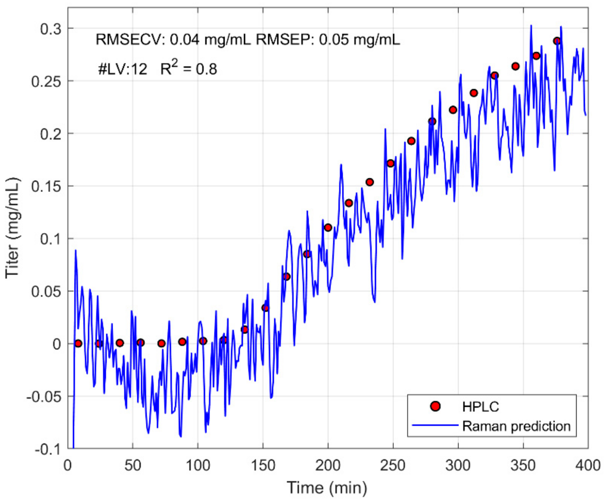
3.1. Partial Least Squares Raman Modeling

The acquired Raman spectra of the BT curves are comparable with the spectra described in [10] and are shown in Figure S1A. Due to the high impurity content in the harvest, the spectral features of different species (i.e., target mAb, media components, HCPs, DNA and HMW) overlapped, leading to broad bands and no distinct peak profiles within single spectra. Hence, only small variations between different spectra could be observed, and a suitable data pretreatment and multivariate model calibration were needed to extract useful information, such as the target protein titer. This had an obvious influence on the spectral appearance shown in Figure S1B. The variable importance in projection (VIP), shown in Figure S1C, indicates the regions between 2300 and 2700 cm⁻¹ as well as between 2900 and 3000 cm⁻¹ as very important. This is in line with the fact that proteins exhibit several Raman bands in the region between 2500–4000 cm⁻¹ [37]. Results of the PLS modeling for different rotations are shown in

Table 3. Data set information and PLS modeling results of all rotations.

	Calibr.set (# Obs)	Pred.set (# Obs)	Opt. num. of LV	RMSECV (mg/mL)	RMSEP (mg/mL)	R2
ROT1	1755	398	12	0.042	0.051	0.80
ROT2	1711	442	12	0.042	0.047	0.86
ROT3	1656	497	12	0.040	0.061	0.78
ROT4	1906	247	12	0.041	0.072	0.70
ROT5	1918	235	11	0.042	0.045	0.84
ROT6	1819	334	12	0.041	0.055	0.82

. Though the number of observations in the calibration set varied slightly between rotations, the optimal number of selected latent variables (LVs) was consistent among rotations and was either 11 or 12. The RMSECV was constant around 0.040 mg/mL on a calibration range from 0 to 0.42 mg/mL and was thus almost independent of the rotation scheme. However, variations in the RMSEP between 0.045 and 0.072 mg/mL as well as varying values of R² between 0.70 and 0.86 indicated slight differences between the BT runs.

The prediction of titer as a function of time for ROT1 is exemplarily shown in Figure 3. The red dots represent the off-line HPLC titer measurements for each fraction, whereas the continuous blue line represents the Raman-PLS-based prediction. It can be seen that the trend of the BT curve was generally well captured by Raman. However, the predictions were clearly scattered around the reference values. It is worth mentioning that increasing the number of scans per Raman measurement could improve the signal-to-noise ratio. However, this would extend the measurement duration, which is critical in most of the downstream processing applications.

As for other rotations, shown in Figure 4, one can observe a clear offset of the predictions at the initial phase (i.e., before breakthrough started). In spite of an optimized laser exposure time, signal enhancement through the flow cell and spectral pretreatment methods, the signal-to-noise ratio was rather small and probably close to the detection limit. Though the obtained averaged RMSEP of 0.05 mg/mL and averaged R² of 0.8 is remarkable, one must probably conclude that Raman-PLS is insufficient for a precise monitoring of a breakthrough at such small concentrations.

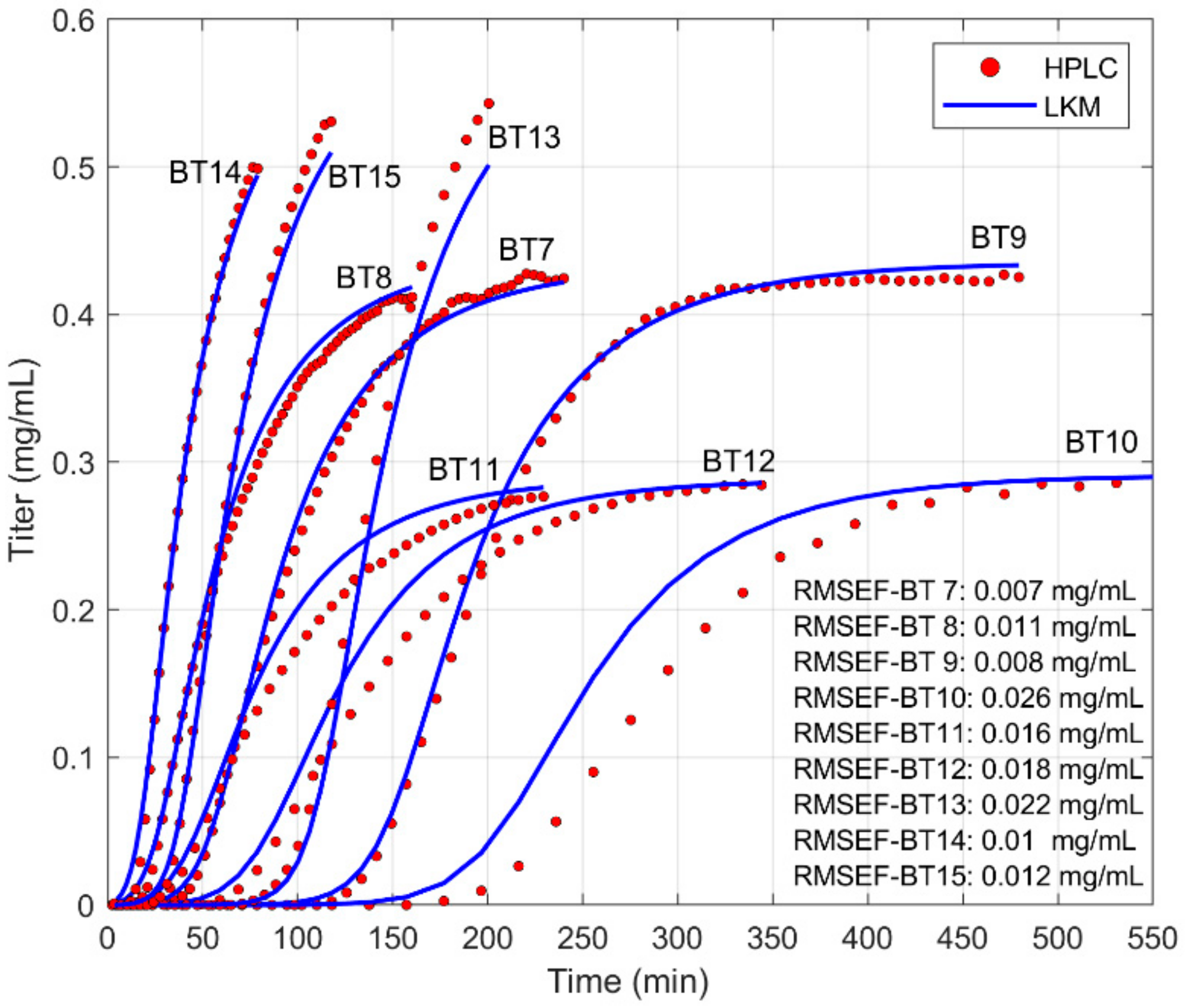
3.2. Mechanistic Modeling

As a next step, an additional set of nine BT runs (BT#7–15) were used to fit the LKM parameters by minimizing the RMSE with the measured concentration values in the breakthrough. The corresponding estimated values (along with 95% confidence intervals) are reported in

Table 4. Fitting parameter of the lumped kinetic model (LKM) optimized on breakthrough (BT)#7–BT#15 ($\epsilon$ = 0.36; $A$ = 17.15; $d_p$ = 85 µm).

$\mathit{H}(-)$	${\mathit{q}}_{\mathit{s}\mathit{a}\mathit{t}}(\mathbf{mg}/\mathbf{mL})$	${\mathit{k}}_{\mathit{m}}^{\mathit{m}\mathit{a}\mathit{x}}\left(\mathbf{min}{-}^1\right)$	${\mathit{S}}_1(-)$	${\mathit{S}}_2(-)$
449.3 ± 31.5	109.7 ± 4.7	8.37 × 10−4 ± 0.94 × 10−4	0.36 ± 0.24	1.76 ± 1.38

and contain the Henry coefficient $H$, saturation capacity $q_{sat}$, the maximum mass transfer coefficient $k_m^{max}$, maximum hindrance coefficient $S_1,$ and the nonlinearity increase of hindrance coefficient $S_2$.

The corresponding model predictions of the breakthrough together with the fitting data sets are shown in Figure 5. The red dots represent the HPLC titer measurements, whereas the continuous blue lines represent the predictions of the LKM. Additionally, the RMSE in fitting (RMSEF) is indicated.

It can be seen that the shapes of BT curves vary in steepness, inflection point and saturation level. This is due to the differences in feed concentration and loading flow rate. At complete column saturation, the asymptotic value of the outlet concentration in the BT tended to the feed concentration. Moreover, higher feed concentrations generally produced earlier breakthroughs. Similarly, larger flow rates not only reduced the residence time in the column but also increased the convection rate along the column with respect to the diffusion rate to the resin, thus producing faster and flatter BT curves. In most cases, the LKM was able to closely predict the trend of the reference measurements. The worst results were obtained in the case of BT#10–12, where RMSEF ranged from 0.016 to 0.026 mg/mL. For such runs, which correspond to the smaller feed concentrations, the error was mostly due to a shift of the predicted BT time with respect to the measured one. In spite of this, it appears that the slope of the predicted BT curves in the inflection point was very similar to the measured one. This result could be explained by an underestimation of the effective column capacity. However, it is difficult to identify the exact origin of this disagreement.

The model ability of predicting new runs was tested by applying the LKM to the first six BT curves (BT#1–6), which were not included in the fitting process of the LKM. The results of the predictions are shown in Figure 6, where the red dots represent HPLC measurements and the blue line the LKM predictions.

It can be observed that the model was able to predict the shape of the BT curves and, in particular, the steepness, indicating a good estimation of the mass transport properties. Additionally, the saturation level seemed to be well predicted, since there is no significant mismatch between estimated and measured times for reaching saturation conditions. However, BT#1–4 showed a significant offset, leading to RMSEP values up to 0.039 mg/mL. This may be related to the fact that the model might not have precisely captured the adsorption mechanism at lower feed concentrations, which could also explain the offsets in Figure 5. Moreover, one can also observe a different behavior in the curves at early BT times. The measured BT curves seem sharper than what was predicted by the model. Again, this might be due to unaccounted differences in the feed composition, resin aging, column packing quality or a more complex behavior of the system than described by the model. Of course, more complex models could be introduced to improve the description of, particularly, the mass transfer process [31,38]. On the contrary, the good ability of the model to predict the shape of the BT curve well in spite of its generality and simplicity makes it a good candidate for its application in the frame of the EKF, where such inaccuracies could be corrected in real-time by experimental measurements.

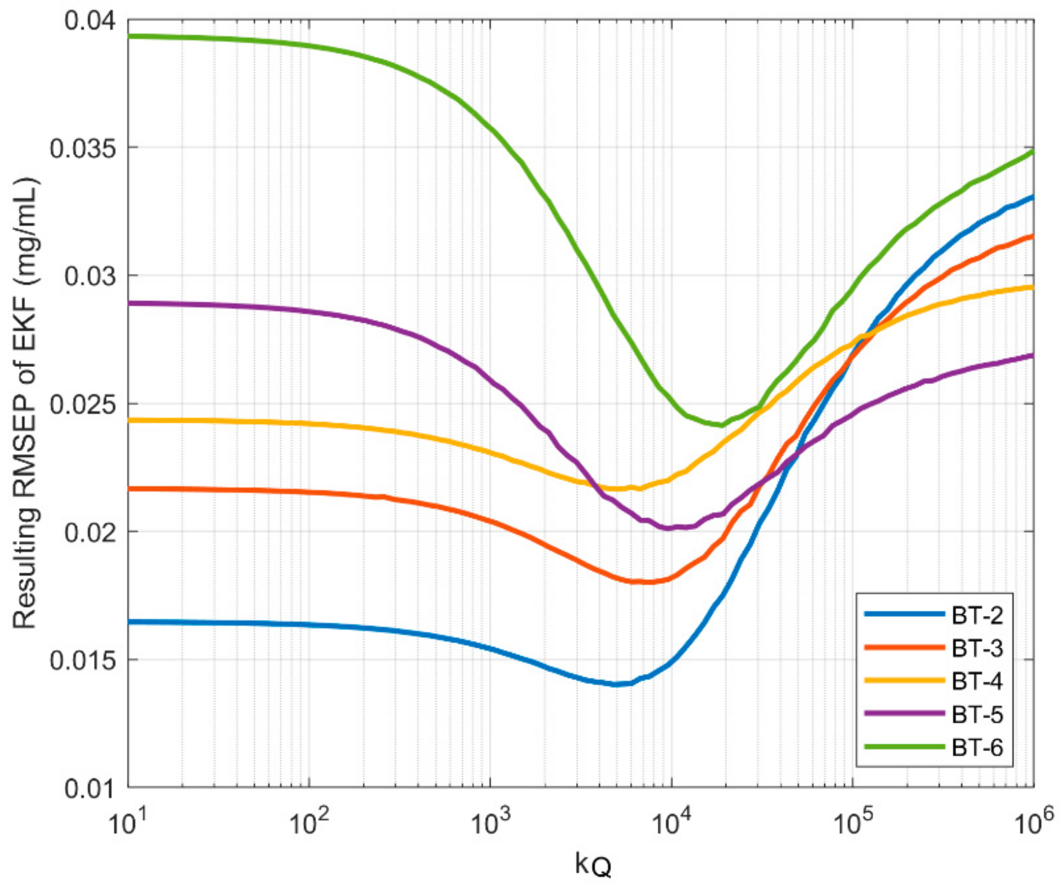
3.3. Extended Kalman Filter Tuning

Before applying the EKF concept, the filter design parameters $R$, $\widehat{x}\left(t_0^{+}\right)$, $Q$ and $k_Q$ needed to be carefully selected and tuned. For this, the variance of the Raman-PLS model ($RMSEC{V}_{PLS}{}^2)$ was used as the measurement noise $R$, while the process noise $Q$ was computed on-line at any given $t_k$, as described in Section 2.6. Since mismatches between the LKM predictions and external data set were expected, a rotation specific mismatch factor $k_Q$ was applied. In the following, the determination of $k_Q$ for ROT1 ($k_Q^{Rot 1})$ is described: The EKF was applied for each BT curve of the calibration set of ROT1, i.e., BT#2–6, using the Raman-PLS calibrated for ROT1, LKM predicting the distinct BT curve and varying $k_Q$ in a range between 10 and 1 × 10⁶. The resulting $RMSE{P}_{EKF}$ as a function of $k_Q$ for each BT curve of the training set is shown in Figure 7.

It can be seen that a minimal $RMSE{P}_{EKF}$ could be obtained by selecting $k_Q$ around 1 × 10⁴ for all BT curves. Note that $k_Q$ can be regarded as a measure of the confidence in Raman measurements versus the confidence in the mechanistic model. The higher $k_Q,$ the more the EKF relied on Raman-PLS, while for small $k_Q$, the LKM was considered as more trustworthy. It is also important to note that the absolute value of $k_Q$ depended strongly on the absolute values of the estimation of both measurement and process noise. The presence of the minimum in the middle of the investigated $k_Q$ range indicates the beneficial effect of considering both types of information in producing the estimates, thus indicating that this approach is better than using only the LKM (small $k_Q$) or the Raman-PLS model (large $k_Q$). It can be assumed that by further increasing $k_Q$ above 1 × 10⁶, even higher RMSEP could be obtained, since the filter would singly rely on Raman-PLS. In contrast, when $k_Q$ tended towards 10, it singly relied on the LKM. This procedure was repeated for all rotations, and the resulting rotation-specific model mismatch factors ($k_Q^{Rot i})$ are summarized in

Table 5. Rotational specific model mismatch factor $k_Q^{Rot i}$ for all rotations.

	ROT1	ROT2	ROT3	ROT4	ROT5	ROT6
$k_Q^{Rot i}$	1.35 × 104	1.92 × 104	1.92 × 104	2.15 × 104	1.92 × 104	1.07 × 104

. It can be seen that the values of $k_Q^{Rot i}$ were similar for all rotations, thus indicating a robust confidence balancing between Raman-PLS and LKM predictions.

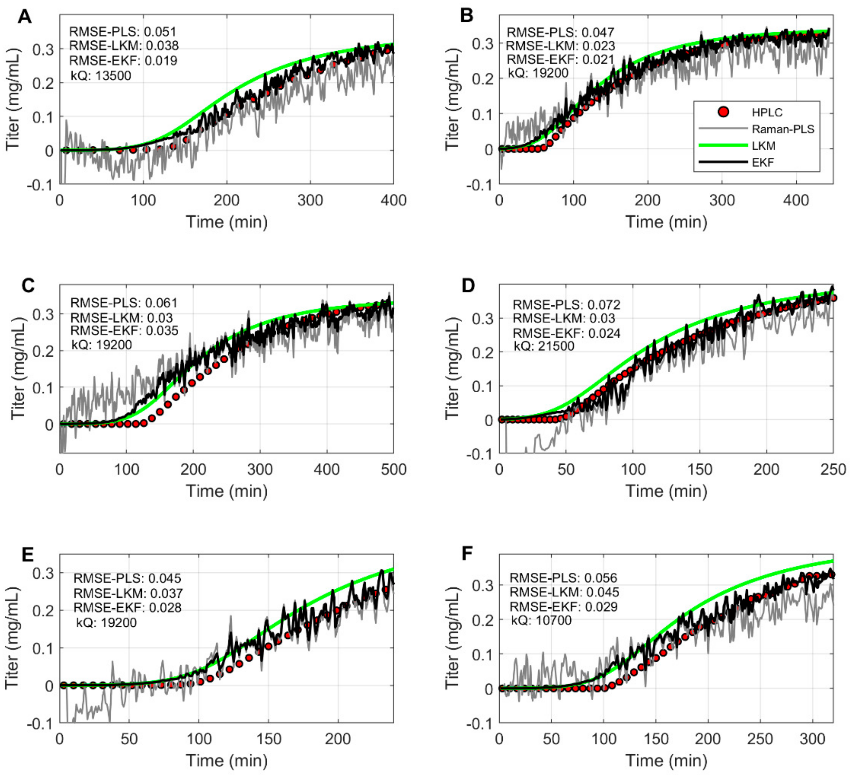
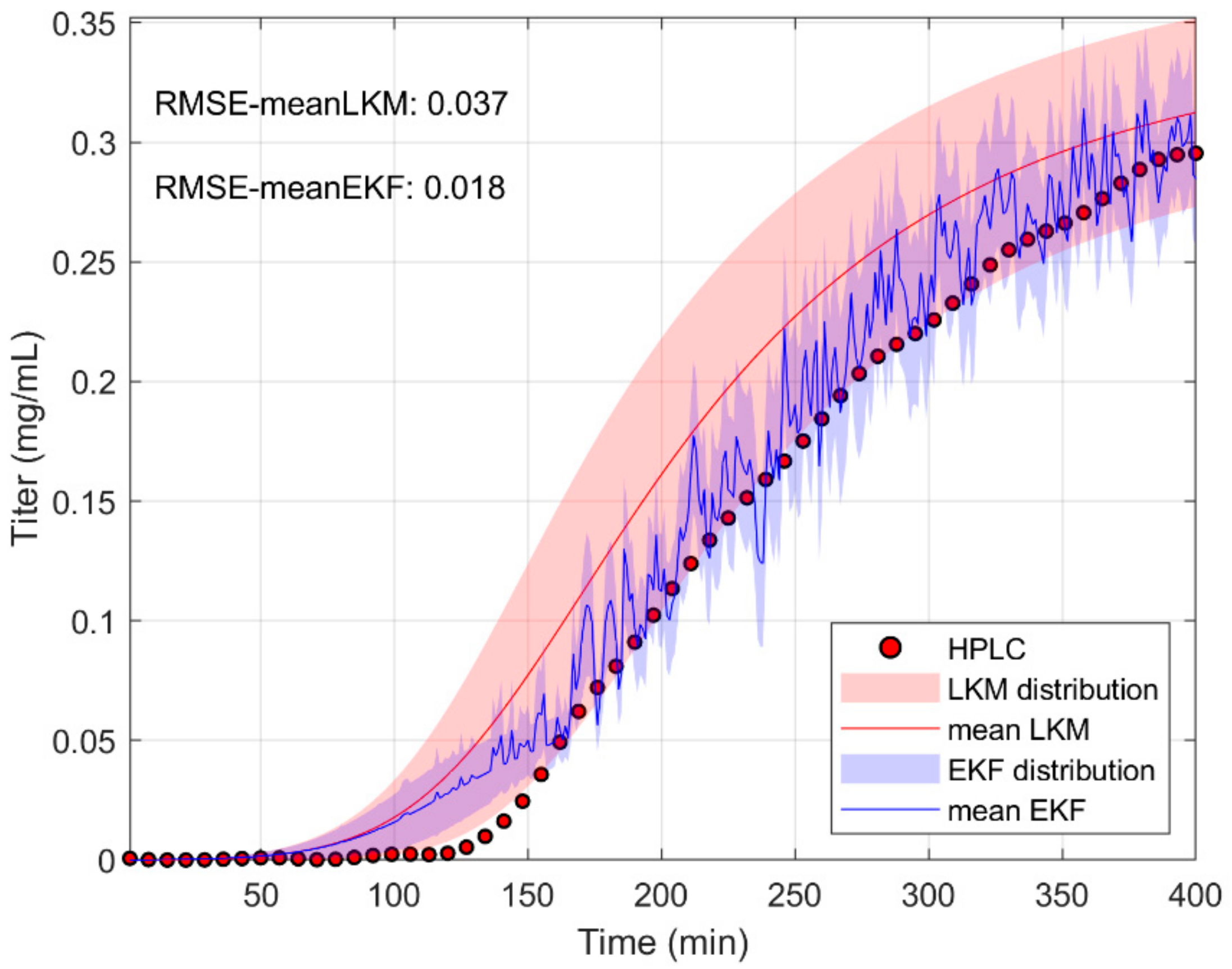
3.4. Extended Kalman Filter Validation

To externally validate the EKF, the rotational approach explained in Section 2.6 and Table 2, was applied for all rotations. In Figure 4A–F, the final results of Raman-PLS, the LKM and EKF for ROT1-6 are shown, respectively.

The red dots represent the off-line HPLC measurements; the continuous grey and green lines represent the Raman-PLS and LKM predictions, respectively; the black line represents the results of the EKF. As mentioned above, the Raman-PLS predictions showed significant noise, although they captured the trend of the actual BT curve. A significant prediction offset can be seen in ranges at the beginning of the breakthrough. Here, the Raman-PLS prediction was rather untrustworthy, which might be explained through difficulties in training the model on samples which did not contain the target molecule or contained a very small amount of it, close to the limit of detection. On the other hand, the LKM was able to smoothly predict the shape of the BT curve, although it showed a constant and significant error. As also noted before, the LKM tended to anticipate the onset of breakthrough, which appeared sharper in the experiments. The line of the EKF seemed, as expected, to be a combination of the curves above, with the beneficial effect of eliminating the mechanistic model offsets on one hand and smoothening the high noise of the Raman predictions on the other. The EKF was particularly reliable in the region of the incipient breakthrough, where its predictions relied mostly on the LKM results, thus eliminating the negative concentration values predicted by the Raman-PLS. On the other hand, at concentration values of 0.1 mg/mL, the offset with respect to the off-line measurements was eliminated and simultaneously reduced the noise. This same pattern exists in all other rotations, as seen by the data summarized in

Table 6. Prediction errors of the Raman-PLS, the LKM and EKF model for all rotations.

	Raman-PLS RMSEP (mg/mL)	LKM RMSEP (mg/mL)	EKF RMSEP (mg/mL)
ROT1	0.051	0.038	0.019
ROT2	0.047	0.023	0.021
ROT3	0.061	0.030	0.035
ROT4	0.072	0.030	0.024
ROT5	0.045	0.037	0.028
ROT6	0.055	0.045	0.029
Mean:	0.055	0.034	0.026

, where the errors in terms of RMSEP for Raman-PLS, LKM and EKF predictions are compared for all considered rotations.

As can be observed in Table 6, the RMSEP_PLS and RMSEP_LKM could be reduced by applying the EKF. The only exception to this trend was ROT3, where the LKM was slightly better. In this case, both the Raman-PLS and the LKM both largely anticipated the BT time. Nevertheless, the advantage of using an EKF estimator appears very clear from this table, especially in significantly reducing the error of those rotations exhibiting a large Raman-PLS model error.

3.5. Extended Kalman Filter Perturbation

One of the major drawbacks of the LKM approach is its sensitivity to the input process parameters. This is illustrated in Figure 8 with reference to ROT1, where the effect of a 5% Gaussian distributed perturbation in feed concentration and flow rate, as well as bed porosity on the predictions of the LKM and the EKF, is compared for 200 simulations. The selected perturbed process parameters are representative of the variables that are actually subject to perturbations in real applications.

The solid line indicates the mean of the predictions of all 200 simulations using the LKM (red) and EKF (blue), whereas the shaded areas show the corresponding 68% confidence intervals, respectively. While the red shaded area is broad and clearly deviates from the reference off-line HPLC measurements, the blue shaded area is rather narrow and distributed around the reference values. It can be concluded that the LKM was strongly affected by perturbations of its input parameters, while this sensitivity was reduced for the EKF predictions due to the influence of the Raman-based estimates.

4. Conclusions

In this work, an EKF estimator of the monoclonal antibody concentration at the outlet of a chromatographic column was developed. Its predictions considerably improved with respect to the use of the single Raman-PLS or the LKM. This was demonstrated for the case of a low titer harvest (mAb conc. < 0.42 mg/mL), which is typical for perfusion bioreactors. In general, the PLS-based predictive Raman models were able to capture the shape of the breakthrough curves, but the obtained results were too noisy for practical applications—for example, in the direction of process control. On the other hand, the mechanistic LKM, properly tuned on an external data set, was able to capture the qualitative shape of the breakthrough curves, but it exhibited deviations that were too large with respect to the off-line reference measurements. The proper application of the EKF requires the preliminary estimation of the parameter $k_Q$, which is responsible for weighting the contribution of the Raman-PLS and the LKM predictions in the final estimate of the filter. By applying the tuned EKF to an external data set, its superiority as compared to Raman-PLS and LKM became obvious. While the LKM predictions served as a solid backbone for the EKF, the Raman-PLS real-time information updated the state estimates and significantly reduced the LKM offset. Though the LKM showed, in some cases, comparable prediction errors, the perturbation analysis showed the additional benefit of EKF through the increased robustness with respect to the model input parameter values. It is worth noting that the RMSE-EKF of 0.026 mg/mL on a range of 0–0.42 mg/mL is very close to the analytical standard deviation of the reference off-line HPLC measurements (0.01 mg/mL). However, it needs to be mentioned that the low detection limit of Raman spectroscopy becomes critical at very low protein concentrations. Here, the LKM could of course be of help, and the EKF predictions should rely mostly on these values. To fully benefit from the LKM, it should be specifically tuned in the region of low concentrations, which is at the incipient breakthrough. Nevertheless, the EKF performance reported in this work is already sufficient for the implementation in the frame of the control of a capture chromatographic step, where the range of interest is around 70% of the breakthrough value [39]. It can be concluded that the EKF is a powerful tool for smart sensors and should be considered more often for monitoring and control within bioprocesses. In the future, this approach might be extended to other applications where deterministic knowledge is available, like in the monitoring of protein aggregation [40], crystallization [41] or in-line buffer preparation. At the same time, research activities on the different components of a Raman analyzer towards increased signal intensities should be continued to further increase the prediction accuracy and reduce the measurement duration.

References

1. Glassey, J.; Gernaey, K.V.; Clemens, C.; Schulz, T.W.; Oliveira, R.; Striedner, G.; Mandenius, C.-F. Process Analytical Technology (PAT) for Biopharmaceuticals. Biotechnol. J. 2011, 6, 369–377. [Google Scholar] [CrossRef] [PubMed]
2. Rathore, A.S.; Bhambure, R.; Ghare, V. Process Analytical Technology (PAT) for Biopharmaceutical Products. Anal. Bioanal. Chem. 2010, 398, 137–154. [Google Scholar] [CrossRef] [PubMed]
3. Simon, L.L.; Pataki, H.; Marosi, G.; Meemken, F.; Hungerbühler, K.; Baiker, A.; Tummala, S.; Glennon, B.; Kuentz, M.; Steele, G.; et al. Assessment of Recent Process Analytical Technology (PAT) Trends: A Multiauthor Review. Org. Process Res. Dev. 2015, 19, 3–62. [Google Scholar] [CrossRef]
4. Read, E.K.; Park, J.T.; Shah, R.B.; Riley, B.S.; Brorson, K.A.; Rathore, A.S. Process Analytical Technology (PAT) for Biopharmaceutical Products: Part I. Concepts and Applications. Biotechnol. Bioeng. 2010, 105, 276–284. [Google Scholar] [CrossRef] [PubMed]
5. Sommeregger, W.; Sissolak, B.; Kandra, K.; von Stosch, M.; Mayer, M.; Striedner, G. Quality by control: Towards model predictive control of mammalian cell culture bioprocesses. Biotechnol. J. 2017, 12, 1600546. [Google Scholar] [CrossRef] [PubMed]
6. Rüdt, M.; Briskot, T.; Hubbuch, J. Advances in Downstream Processing of Biologics—Spectroscopy: An Emerging Process Analytical Technology. J. Chromatogr. A 2017, 1490, 2–9. [Google Scholar] [CrossRef] [PubMed]
7. Santos, R.M.; Kessler, J.-M.; Salou, P.; Menezes, J.C.; Peinado, A. Monitoring MAb cultivations with in-situ raman spectroscopy: The influence of spectral selectivity on calibration models and industrial use as reliable PAT tool. Biotechnol. Prog. 2018, 34, 659–670. [Google Scholar] [CrossRef] [PubMed]
8. Berry, B.; Moretto, J.; Matthews, T.; Smelko, J.; Wiltberger, K. Cross-scale predictive modeling of CHO cell culture growth and metabolites using raman spectroscopy and multivariate analysis. Biotechnol. Prog. 2015, 31, 566–577. [Google Scholar] [CrossRef]
9. Craven, S.; Whelan, J.; Glennon, B. Glucose concentration control of a fed-batch mammalian cell bioprocess using a nonlinear model predictive controller. J. Process Control 2014, 24, 344–357. [Google Scholar] [CrossRef]
10. Feidl, F.; Garbellini, S.; Vogg, S.; Sokolov, M.; Souquet, J.; Broly, H.; Butté, A.; Morbidelli, M. A new flow cell and chemometric protocol for implementing in-line raman spectroscopy in chromatography. Biotechnol. Prog. 2019. [Google Scholar] [CrossRef]
11. Buckley, K.; Ryder, A.G. Applications of Raman spectroscopy in biopharmaceutical manufacturing: A short review. Appl. Spectrosc. 2017, 71, 1085–1116. [Google Scholar] [CrossRef] [PubMed]
12. Esmonde-White, K.A.; Cuellar, M.; Uerpmann, C.; Lenain, B.; Lewis, I.R. Raman spectroscopy as a process analytical technology for pharmaceutical manufacturing and bioprocessing. Anal. Bioanal. Chem. 2017, 409, 637–649. [Google Scholar] [CrossRef] [PubMed]
13. Lewis, I.R. Handbook of Raman Spectroscopy; CRC Press: Boca Raton, FL, USA, 2001. [Google Scholar] [CrossRef]
14. Guiochon, G. Preparative liquid chromatography. J. Chromatogr. A 2002, 965, 129–161. [Google Scholar] [CrossRef]
15. Auger, F.; Hilairet, M.; Guerrero, J.M.; Monmasson, E.; Orlowska-Kowalska, T.; Katsura, S. Industrial applications of the Kalman Filter: A Review. IEEE Trans. Ind. Electron. 2013, 60, 5458–5471. [Google Scholar] [CrossRef]
16. Krämer, D.; King, R. On-line monitoring of substrates and biomass using near-infrared spectroscopy and model-based state estimation for enzyme production by S. cerevisiae. IFAC PapersOnLine 2016, 49, 609–614. [Google Scholar] [CrossRef]
17. Stelzer, I.V.; Kager, J.; Herwig, C. Comparison of particle filter and extended kalman filter algorithms for monitoring of bioprocesses. In Computer Aided Chemical Engineering; Elsevier: Amsterdam, The Netherlands, 2017; Volume 40, pp. 1483–1488. [Google Scholar] [CrossRef]
18. Arndt, M.; Hitzmann, B. Kalman Filter Based Glucose Control at Small Set Points during Fed-Batch Cultivation of Saccharomyces Cerevisiae. Biotechnol. Prog. 2008, 20, 377–383. [Google Scholar] [CrossRef]
19. Kalman, R.E. A new approach to linear filtering and prediction problems. J. Basic Eng. 1960, 82, 35. [Google Scholar] [CrossRef]
20. Faragher, R. Understanding the Basis of the Kalman Filter Via a Simple and Intuitive Derivation [Lecture Notes]. IEEE Signal Process. Mag. 2012, 29, 128–132. [Google Scholar] [CrossRef]
21. Simon, D. THE H∞ FILTER. In Optimal State Estimation; John Wiley & Sons, Inc.: Hoboken, NJ, USA, 2006; pp. 331–371. [Google Scholar] [CrossRef]
22. Wolf, M.K.F.; Müller, A.; Souquet, J.; Broly, H.; Morbidelli, M. Process design and development of a mammalian cell perfusion culture in shake-tube and benchtop bioreactors. Biotechnol. Bioeng. 2019, 116, 1973–1985. [Google Scholar] [CrossRef]
23. Feidl, F.; Vogg, S.; Wolf, M.K.F.; Podobnik, M.; Ruggeri, C.; Ulmer, N.; Wälchli, R.; Souquet, J.; Broly, H.; Butte, A.; et al. Process-Wide Control and Automation of an Integrated Continuous Manufacturing Platform for Therapeutic Proteins. Submiss 2019. submitted for publication. [Google Scholar]
24. Savitzky, A.; Golay, M.J.E. Smoothing and Differentiation of Data by Simplified Least Squares Procedures. Anal. Chem. 1964, 36, 1627–1639. [Google Scholar] [CrossRef]
25. Barnes, R.J.; Dhanoa, M.S.; Lister, S.J. Standard normal variate transformation and de-trending of near-infrared diffuse reflectance spectra. Appl. Spectrosc. 1989, 43, 772–777. [Google Scholar] [CrossRef]
26. Van den Berg, R.A.; Hoefsloot, H.C.; Westerhuis, J.A.; Smilde, A.K.; van der Werf, M.J. Centering, scaling, and transformations: Improving the biological information content of metabolomics data. BMC Genom. 2006, 15, 1–15. [Google Scholar] [CrossRef]
27. Wold, S.; Sjöström, M.; Eriksson, L. PLS-Regression: A Basic Tool of Chemometrics. Chemom. Intell. Lab. Syst. 2001, 58, 109–130. [Google Scholar] [CrossRef]
28. Kohavi, R. A study of cross-validation and bootstrap for accuracy estimation and model selection. IJCAI 1995, 14, 1137–1145. [Google Scholar]
29. Baur, D.; Angarita, M.; Müller-Späth, T.; Morbidelli, M. Optimal model-based design of the twin-column capturesmb process improves capacity utilization and productivity in protein A affinity capture. Biotechnol. J. 2016, 11, 135–145. [Google Scholar] [CrossRef] [PubMed]
30. Hahn, R.; Schlegel, R.; Jungbauer, A. Comparison of protein A affinity sorbents. J. Chromatogr. B 2003, 790, 35–51. [Google Scholar] [CrossRef]
31. Guiochon, G.; Shirazi, D.G.; Felinger, A.; Katti, A.M. Fundamentals of Preparative and Nonlinear Chromatography; Academic Press: Cambridge, MA, USA, 2006. [Google Scholar]
32. Ng, C.K.S.; Osuna-Sanchez, H.; Valéry, E.; Sørensen, E.; Bracewell, D.G. Design of high productivity antibody capture by protein A chromatography using an integrated experimental and modeling approach. J. Chromatogr. B 2012, 899, 116–126. [Google Scholar] [CrossRef] [Green Version]
33. Valappil, J.; Georgakis, C. Systematic estimation of state noise statistics for extended kalman filters. AIChE J. 2000, 46, 292–308. [Google Scholar] [CrossRef]
34. Schneider, R.; Georgakis, C. How to not make the extended Kalman filter fail. Ind. Eng. Chem. Res. 2013, 52, 3354–3362. [Google Scholar] [CrossRef]
35. Kuo, A.D. An optimal state estimation model of sensory integration in human postural balance. J. Neural Eng. 2005, 2, S235–S249. [Google Scholar] [CrossRef] [PubMed]
36. Jazwinski, A.H. Stochastic Processes and Filtering Theory; Courier Corporation: North Chelmsford, MA, USA, 2007. [Google Scholar]
37. Wen, Z. Raman Spectroscopy of Protein Pharmaceuticals. J. Pharm. Sci. 2007, 96, 2861–2878. [Google Scholar] [CrossRef] [PubMed]
38. Carta, G.; Jungbauer, A. Protein Chromatography; Wiley: Weinheim, Germany, 2010. [Google Scholar] [CrossRef]
39. Steinebach, F.; Angarita, M.; Karst, D.J.; Müller-Späth, T.; Morbidelli, M. Model based adaptive control of a continuous capture process for monoclonal antibodies production. J. Chromatogr. A 2016, 1444, 50–56. [Google Scholar] [CrossRef] [PubMed]
40. Nicoud, L.; Owczarz, M.; Arosio, P.; Morbidelli, M. A multiscale view of therapeutic protein aggregation: A colloid science perspective. Biotechnol. J. 2015, 10, 367–378. [Google Scholar] [CrossRef] [PubMed]
41. Rupp, B. Predictive models for protein crystallization. Methods 2004, 34, 390–407. [Google Scholar] [CrossRef] [PubMed]
Figure 1. Schematic illustration of the developed flow cell.
Processes 07 00683 g001
Figure 2. Schematic illustration of the experimental set up to perform chromatographic breakthrough runs and collecting synchronized Raman measurements and breakthrough fractions.
Processes 07 00683 g002
Figure 3. Time evolutions of Raman-PLS predictions (blue) for rotation 1 (ROT1) compared to off-line HPLC measurements (red).
Processes 07 00683 g003
Figure 4. Titer predictions of Raman-PLS (grey), the LKM (green), the EKF model with tuned k Q (black) and HPLC off-line measurements (red) for rotations 1–6 (AF).
Processes 07 00683 g004
Figure 5. Internal mechanistic model (LKM) predictions of titer for BT#7–15 (blue) and corresponding HPLC off-line measurements (red).
Processes 07 00683 g005
Figure 6. Mechanistic model (LKM) predictions of titer for BT# 1–6 with parameter values fitted on BT# 7–15 (blue) compared to HPLC off-line measurements (red).
Processes 07 00683 g006
Figure 7. Error in the EKF prediction of the monoclonal antibody (mAb) concentration as a function of the model mismatch factor k Q for each of the BT curves of the calibration set of ROT1.
Processes 07 00683 g007
Figure 8. Effect of 5% Gaussian distributed perturbations in feed concentration and flow rate, as well as bed porosity on the predictions of the LKM (mean = dark red; standard deviation interval = light red) and the EKF (mean = dark blue; standard deviation interval = light blue) of ROT1 in 200 simulations.
Processes 07 00683 g008