Diagnostics-Oriented Modelling of Micro Gas Turbines for Fleet Monitoring and Maintenance Optimization

Abstract

The market for the small-scale micro gas turbine is expected to grow rapidly in the coming years. Especially, utilization of commercial off-the-shelf components is rapidly reducing the cost of ownership and maintenance, which is paving the way for vast adoption of such units. However, to meet the high-reliability requirements of power generators, there is an acute need of a real-time monitoring system that will be able to detect faults and performance degradation, and thus allow preventive maintenance of these units to decrease downtime. In this paper, a micro gas turbine based combined heat and power system is modelled and used for development of physics-based diagnostic approaches. Different diagnostic schemes for performance monitoring of micro gas turbines are investigated.

1. Introduction

According to multiple sources, the global market for micro gas turbine (MGT) will experience an expeditious growth in the coming years [1,2,3]. The power generation segment of its product portfolio is expected to contribute to a bulk portion of this growth. In particular, the combined heat and power (CHP) configuration of this energy generator are grabbing much attention from both the industry and the policy makers [4,5]. Especially in the context of European Unions’(EU) initiatives against climate change, these micro-CHP units could play a vital role in achieving both short- and long-term emission reduction targets.

MGTs are gas turbines combined with high speed generators whose electrical output can range between few kilowatts and few hundreds kilowatts. They offer a number of benefits compared to other technologies for distributed heat and power generation, including compact size, lightweight, fewer moving parts, lower maintenance needs, lower noise and vibration, high reliability, higher fuel flexibility, lower emission levels, potential for low cost mass production, and potential for integration with others decentralised energy generators [6,7,8,9]. On the other hand, the main drawbacks of MGTs are low electrical efficiency, high research and development cost, and high ownership cost at the moment [5,7]. However, numerous development activities are under-way by academia, industry, and policy makers to overcome the aforementioned challenges.

To bring the cost of ownership down, multiple vendors are offering micro-CHP units that are being developed by utilizing commercial off-the-shelf (COTS) components from automotive turbocharger industry. The inclusion of mature turbocharger technology offers not only cost reduction, but also high reliability and robustness that the industry achieved through decades of continuous improvement. On the contrary, turbochargers are not optimised for MGT operation due to the trade-off between design point efficiency and cost of manufacturing. For this reason, the MGT market is still considered to be a niche market, and the cost for development of turbo-machinery optimised for MGT operation can only be justified with mass production. Hence, modification of automotive turbocharger is often preferred to improve design point efficiency.

In the context of a power sector with high share of intermittent energy sources, MGTs should offer high reliability and availability to ensure the security of supply. Subsequently, an on-line condition-based monitoring and fault detection system is necessary. MGT runtime can be extended by early detection of faults and performance degradation. Thus, it will be possible to plan maintenance activity long before a breakdown occurs. Eventually, this will improve the availability and lower the maintenance cost. Another important aspect of future MGT market that emphasises the need of a condition-based monitoring and fault detection system is the ownership structure. Traditionally, gas turbines are owned by utilities and large companies. However, MGT-based CHP units could also be owned by private persons and small and medium enterprises (SME). Hence, a service-oriented approach is vital, where the service provider (i.e., technology provider or system installer or independent service provider) might need to manage a large fleet of MGT units. This is where the concept of fleet level monitoring and diagnostics can play an important role. The service provider will be responsible for monitoring the MGT fleet and planning maintenance based on the engine health conditions and severity of deterioration. Hence, an integrated approach for MGT fleet monitoring and diagnostics is necessary to foster the adoption of this promising technology. Since the MGT technology is still in the early stage of commercialization phase, sufficient data on degraded and faulty operations are lacking, which rules out the use of data-driven diagnostics approaches for the moment. Moreover, data-driven approaches perform worse for cases that fall outside of the training dataset, which could be a limitation considering the wide operating flexibility that is expected from MGT units. Therefore, physics-based modelling for MGT diagnostics appears necessary to overcome the aforementioned challenges.

Realizing its potential, the exploitation of a physics-based model for MGT fleet monitoring and diagnostics is investigated in this paper. A diagnostic-oriented model for an MGT based CHP unit is developed. An in-house Fortran-based gas turbine modelling tool named EnVironmental Assessment (EVA) is used for model development [10,11]. Model adaptation techniques for individual MGT units in a fleet are also discussed in detail. Subsequently, a multi-level fault detection and isolation methods are presented along with a detailed fault diagnostics scheme that can identify the location and magnitude of different component faults. Finally, several simulation trials are performed to test the presented fault diagnostics scheme.

2. Review on Performance Based Gas Path Diagnostics

The performance of gas turbines deteriorates over time, leading to reduced output capacity and thermal efficiency that in turn result in reduced profitability and increased emissions [12]. Generally, any performance deterioration in a gas turbine can be linked with performance deterioration of one or more gas path components. The performance of these components deteriorate over time due to various degradation mechanisms such as fouling, erosion, corrosion, internal liner surface cracking, increase in tip and seal clearance, foreign object damage, plugging of the injector and the cooling holes, etc. [13,14,15]. The rate at which these deterioration mechanisms take place could be different depending on the manufacturing tolerance, engine operating conditions, operating regime, i.e., part or full load, start-stop cycles, and fuel type and quality. Deterioration generally causes deviations in the component performance parameters, i.e., efficiency, pressure ratio, flow capacity, and others, which in turn lead to deviations in the gas path measurable parameters such as temperatures, pressures, speed, and flow rates. Using the gas path measurable parameters to detect the change in component health parameters forms the foundation for performance-based gas path analysis (GPA) methods for gas turbine diagnostics. Two of the well-known variants of this method are physics-based and data-driven GPA. Numerous comprehensive review articles explore existing GPA approaches (both physics-based and data-driven) and their relative performance [16,17,18,19,20]. In these articles, the comparative pros and cons of different approaches are examined based on attributes such as reliability, accuracy, model complexity, computational efficiency, the ability to cope with noise and bias, and number of measurements required for diagnostics. The findings of these reviews can be summarized by stating that there is no single approach that outperforms the others in all the attributes; rather they are complementary and each has its own benefits and drawbacks. Hence, hybrid schemes that combine both physics-based and data-driven approaches should be preferred. As a starting point for MGT diagnostics and in light of the limitations previously discussed, the focus of this study is limited to a physics-based approach.

Physics-based GPA approaches for gas turbines diagnostics have been widely studied by the research community over the years. As the name suggests, these approaches explicitly rely on the physics-based models of gas turbines. The models are based on mathematical and thermodynamic equations that principally correlate gas path measurable parameters with component performance parameters. The has approach developed much since Urban pioneered it in 1967 [21]. Urban [22,23] and others [24,25,26] further investigated the approach, which is widely referred to as linear GPA in the literature. In linear GPA, unknown variations in components performance parameters are computed from known variations in measurable parameters by using a set of linear equations. The equations are derived by linearising the non-linear equations that link components performance parameters with measurable parameters, around a specific steady-state operating point. Being conceptually simple and computationally light, linear GPA offers numerous benefits such as fault isolation and quantification and multiple faults diagnostics. On the other hand, the method has multiple limitations. It requires many relevant measurements for fault diagnostics, which can be quite rare in commercial units. Due to the assumption of linearity, the method shows instability and large inaccuracy under higher level of deteriorations. Moreover, it is unable to deal with sensor noise and bias.

To cope with the non-linear behaviour of the gas turbines and improve the accuracy of GPA, non-linear GPA was introduced by House [27] and Esher [28]. The method was further improved by many others. Unlike linear GPA, in non-linear GPA, the full equations are treated directly without any linearisation. To deal with the engine to engine variations, an adaptive approach of non-linear GPA was examined by Stamatis et al. [29]. The author introduced modification factors to the health parameters to take care of the individual engine variation that are computed through an optimisation procedure. Li [30] developed a two step approach for linear and non-linear adaptive GPA that can detect both single and simultaneously occurring multiple faults. Not long ago, Larsson [31] presented a systematic design procedure to construct a fault detection and isolation system by using complex non-linear models. In a more recent work, Liu [32] proposed a dynamic tracking filter incorporating state observer to detect the variation of six performance parameters of three gas path components by using four measurement parameters. However, the usage of linear state observer resulted in reduced accuracy in fault detection capability of this approach; hence, a non-linear state observer is required. In another work, Kang [33] suggested a compressor map adaptation technique to enhance the accuracy of performance based diagnostics of a heavy-duty gas turbine. Comparison of different diagnostics approaches are studied in Koskoletos et al. [34]. The authors performed a comparative analysis among: (1) probabilistic neural network (PNN); (2) k-nearest neighbours; (3) optimization; (4) combinatorial; (5) adaptive 2X2; and (6) combination of PNN and adaptive 2X2 method. They concluded that Methods 3–6 can be used for component fault magnitude estimation and prognostic purpose.

Previous research efforts have made valuable contributions in improving performance-based gas path diagnostics methods. However, most of this work is focused on large scale industrial gas turbines; only a few studies are focused on micro gas turbine [35,36,37,38]. Performance-based diagnostics of MGT by employing GPA poses numerous challenges. To keep the cost of ownership down, MGTs include only few measurements of gas path parameters. Moreover, some of these measurements are used for control purpose, meaning that they cannot be utilized for diagnostics. Due to the high manufacturing tolerances, engine components show wide variations in performance, which could lead to deviations in measured parameters that are comparable to fault conditions. Hence, model tuning is essential for individual engines before employing any fault diagnostics approach.

3. Methodology

To develop a model-based diagnostics scheme for an MGT fleet, a diagnostics-oriented model of a nominal MGT unit is developed and presented in this article. The developed model is validated against the measurements from the performance test of a commercial MGT unit. Sequentially, a scheme for model tuning is employed to account for engine to engine variations. Finally, a diagnostics scheme is proposed and tested with the help of simulation studies.

3.1. Gas Path Modelling of the Micro Gas Turbine

The operating principle of an MGT is identical to large-scale open cycle gas turbines. Both operate on the well-known Brayton cycle. As shown in Figure 1, a typical MGT with CHP configuration consists of a compressor, a recuperator, combustor, a turbine, a high-speed generator, and an exhaust recovery heat exchanger. The air is compressed in the compressor and then preheated by the exhausts in the recuperator before being further heated by burning fuel in the combustor. The high temperature working fluid is then expanded in the turbine that operates the compressor and the high-speed generator. The remaining exhaust heat is recovered by water in the recovery heat exchanger.

The MGT unit under study in this paper is the EnerTwin Micro-CHP that is marketed by Micro Turbine Technology (MTT) B.V. It is a single-shaft, radial, recuperated gas turbine manufactured in CHP configuration. The micro-CHP unit have a capacity of 3.2 kW of electric and 16 kW thermal output.

A modular modelling technique is employed here to develop the MGT model. All the gas path components, i.e., compressor, recuperator, combustor and turbine including duct and rotating shaft are modelled and integrated just like the way they are connected in reality. As mentioned previously, the MGT model is developed by using an in-house Fortran-based gas turbine modelling tool called EVA. It is a multidisciplinary conceptual design tool that comprises various modules incorporating substantial detail within a wide range of disciplines, i.e., gas turbine performance, aerodynamic and mechanical design, emissions prediction, and environmental impact. In this work, the gas turbine performance analysis module of the tool is utilized.

The compressor and turbine models are based on their corresponding characteristic maps provided by the manufacturer and standard mass and energy balance equations. The characteristics maps provide correlations between pressure ratio ($PR$), shaft speed (N), mass flow rate ($\dot{m}$), and isentropic efficiency (${\eta }_{is}$), as shown in Equation (1).

$$\left(\frac{\dot{m}·\sqrt{T_{in}}}{P_{in}},{\eta }_{is}\right)=f\left(PR,\frac{N}{\sqrt{T_{in}}}\right)$$

(1)

where $T_{in}$ and $P_{in}$ refer to the inlet temperature and pressure respectively. For a known shaft speed and pressure ratio, corresponding mass flow rate and isentropic efficiency are extracted from the characteristic maps. The extracted values are then used in well-known thermodynamic equations to calculate parameters related to compressor and turbine. For example, compressor outlet temperature ($T_2$), pressure ($P_2$), and compression work ($W_{comp.}$) are calculated utilizing Equations (4), (7) and (9).

Starting by assuming isentropic compression and expansion in the compressor and turbine, respectively, the Gibbs equation takes the following form:

$$\underset{=0}{\underbrace{S_{out}-S_{in}}}={\int }_{T_{in}}^{T_{out,is.}}\frac{C_p}{T}·dT-R_g·ln\left(\frac{P_{out}}{P_{in}}\right)$$

(2)

Here, S refers to the entropy, $C_p$ is the specific heat capacity and $R_g$ is the universal gas constant. Defining entropy function as in Equation (3),

$$\varphi \left(T\right)={\int }_{T_{ref.}}^T\frac{C_p}{T}·dT$$

(3)

Equation (4) is derived:

$$\varphi \left(T_{out,is.}\right)=\varphi \left(T_{in}\right)+R_g·ln\left(\frac{P_{out}}{P_{in}}\right)$$

(4)

Here, $\varphi \left(T_{in}\right)$ and $\varphi \left(T_{out,is}\right)$ are the temperature dependent entropy functions at the inlet and outlet of the component (i.e., compressor or turbine).

However, the isentropic assumptions are not applicable to real compression and expansion processes which have inherent losses due to compressor and turbine inefficiencies. To account for these losses, isentropic efficiencies for compressor (${\eta }_{comp.,is.}$) and turbine (${\eta }_{turb.,is.}$) are defined as in Equations (5) and (6).

$${\eta }_{comp.,is.}=\frac{h\left(T_{2,is.}\right)-h\left(T_1\right)}{h\left(T_2\right)-h\left(T_1\right)}$$

(5)

$${\eta }_{turb.,is.}=\frac{h\left(T_5\right)-h\left(T_4\right)}{h\left(T_{5,is.}\right)-h\left(T_4\right)}$$

(6)

Subsequently, compressor and turbine pressure ratios are defined by Equations (7) and (8).

$$P{R}_{comp.}=\frac{P_2}{P_1}$$

(7)

$$P{R}_{turb.}=\frac{P_4}{P_5}$$

(8)

Finally, compressor and turbine works are calculated using Equations (9) and (10),

$$W_{comp.}={\dot{m}}_1\left(h_2-h_1\right)$$

(9)

$$W_{turb.}={\dot{m}}_4\left(h_4-h_5\right)$$

(10)

Here, $\varphi \left(T_1\right)$ and $\varphi \left(T_2\right)$ are the temperature dependent entropy functions at the inlet and outlet of the compressor, and $R_g$ is the universal gas constant.

The recuperator is modelled as a counter-current plate type heat exchanger. Heat exchanger’s key performance parameters related to heat transfer and pressure drop are used for this purpose. The thermal effectiveness ($ϵ$) is used as heat transfer performance parameter, while relative pressure drop in the air-side ($\Delta P_{23}$) and gas-side ($\Delta P_{56}$) are introduced as pressure drop performance parameters. A heat flux-based definition of effectiveness is considered instead of a temperature-based one to include the influence of the gas composition on the specific heat capacity, as shown in Equation (11).

$$ϵ=\frac{Q_{act.}}{Q_{max.}}$$

(11)

$$\Delta P_{23}=\frac{P_3-P_2}{P_2}$$

(12)

$$\Delta P_{56}=\frac{P_6-P_5}{P_5}$$

(13)

where $Q_{act.}$ and $Q_{max.}$ refer to actual heat transfer and maximum possible heat transfer in the recuperator. The maximum possible heat transfer is achieved when the fluid with minimum heat capacity rate undergoes the maximum temperature difference available present in the exchanger, which is the difference in the entering temperatures for the hot and cold fluids.

The combustor performance is given in terms of combustion efficiency (${\eta }_{comb.}$) and relative pressure drop ($\Delta P_{34}$). The combustor efficiency can be computed by Equation (14), while relative pressure drop can be computed using an equation similar to Equation (12). Using these parameters, fuel to air ratio (FAR) and pressure at exit of the combustor ($P_4$) are determined. Finally, energy balance is applied for the combustor to estimate the enthalpy at the combustor outlet that in-turn is used to determine the temperature. For simplicity, a constant lower heating value (LHV) is used in Equation (14).

$${\eta }_{comb.}=\frac{{\dot{m}}_3(h_3-h_2)}{{\dot{m}}_f·LHV}$$

(14)

Compressor, turbine, and generator are mounted on the same shaft; hence, the shaft mechanical efficiency is defined as in Equation (15).

$${\eta }_{shaft}=\frac{W_{comp.}+W_{gen.}}{W_{turb.}}$$

(15)

Pressure losses in the ducts are also taken into account by using an equation similar to Equation (12).

3.1.1. Matching Scheme for Gas Path Modelling

The steady state operating points of the gas turbine are obtained by matching the compressor and turbine. This is done by superimposing turbine map on the compressor map while mass flow and energy continuity are maintained. The serial nested loops method is used where initial guesses are continuously updated until all the residuals error terms, corresponding to components mass and energy balance, reach predefined accuracy. To do this, a Jacobian matrix is built where each element of the matrix is the sensitivity ratio between each output (or target) and state ($\delta Y$/$\delta X$). The Jacobian is used to compute and minimize the residuals between model outputs and targets. In normal conditions, the Jacobian consists of the following pairs of outputs and states in the rows and columns as shown in

Table 1. Jacobian matrix used for modelling (PWX: shaft power).

	States	${\mathit{N}}_{\mathit{rel}.}$	${\dot{\mathit{m}}}_{\mathit{int}.,\mathit{corr}.,\mathit{rel}.}$	${\mathit{\beta }}_{\mathit{comp}.}$	${\mathit{\beta }}_{\mathit{turb}.}$	${\mathit{Q}}_{\mathit{hex}.,\mathit{air},\mathit{nond}.}$	${\mathit{Q}}_{\mathit{hex}.,\mathit{gas},\mathit{nond}.}$	$\mathit{PWX}$	${\dot{\mathit{m}}}_{\mathit{corr}.,\mathit{f},\mathit{rel}.}$
Outputs
$Torqu{e}_{res.}$		0.8978	0.0000	0.7910	0.8590	0.1371	0.0000	0.0001	0.1106
${\dot{m}}_{comp.,res.}$		2.0321	0.9998	0.9557	0.0000	0.0000	0.0000	0.0000	0.0000
${\dot{m}}_{turb.,res.}$		0.4596	0.0000	0.9285	0.0951	0.1412	0.0000	0.0000	0.1102
$Q_{hex.,air,res.}$		0.4589	0.0000	0.0633	0.2508	0.4263	0.0000	0.0000	0.4334
$Q_{hex.,gas,res.}$		0.4589	0.0000	0.0633	0.2508	0.5737	1.0000	0.0000	0.4334
${\dot{m}}_{noz.,res.}$		7.7099	0.0000	1.6493	7.3678	0.0106	0.4625	0.0000	0.0330
$N_{rel,res.}$		1.0000	0.0000	0.0000	0.0000	0.0000	0.0000	0.0000	0.0000
$T_{5,res.}$		0.7408	0.0000	0.6401	0.1407	0.3219	0.0000	0.0000	0.2432

.

For example, the mass continuity in the compressor needs to be satisfied, which means that the mass flow calculated from the compressor map needs to match the compressor inlet mass flow. The speed factor $N_{rel.}$, defined as $N/N_{des.}$, is then varied until the residual between the two mass flow values (${\dot{m}}_{comp.,res.}$ ) is below a predefined defined threshold.

3.1.2. Modified Matching Scheme for Adaptation

For model tuning and gas path diagnostics purpose, correcting factors for the component performance parameters i.e., efficiencies, flow capacities, and effectiveness were included in the MGT model. These factors are included as state variables along with their corresponding target variables. Then, a new Jacobian matrix is built, and new residuals are generated between output variables and target values (

Table 2. Target and state pairs used in the Jacobian matrix for diagnostics (FC: flow capacity).

Targets	States
$Torqu{e}_{res.}$	$N_{rel.}$
${\dot{m}}_{comp.,res.}$	${\dot{m}}_{int.,corr.,rel.}$
${\dot{m}}_{turb.,res.}$	${\beta }_{comp.}$
$Q_{hex.,air,res.}$	${\beta }_{turb.}$
$Q_{hex.,gas,res.}$	$Q_{hex.,air,nond.}$
${\dot{m}}_{noz.,res.}$	$Q_{hex.,gas,nond.}$
$N_{rel,res.}$	$PWX$
$T_{5,res.}$	${\dot{m}}_{corr.,f,rel.}$
$T_{2,res.}$	$\Delta {\eta }_{comp.}$
$P_{2,res.}$	$\Delta F{C}_{comp.}$
$P_{5,res.}$	$\Delta {\eta }_{turb.}$
${\dot{m}}_{1,res.}$	$\Delta F{C}_{turb.}$
$T_{3,res.}$	$\Delta {ϵ}_{rec.}$

) to achieve a solution.

In this case, the standard matching scheme is modified to fit the required state variables. The correcting factor on the flow capacity for compressor and turbine is varied to satisfy the mass flow continuity in these two components. Once the flow capacity is fixed, the beta lines in the compressor and turbine maps are varied to match the desired exit pressure/temperature. The correction factor on the compressor efficiency is varied to match the torque on the shaft, while the speed factor becomes the variable that minimizes the residual between produced power and load demand.

3.2. Scheme for the Model Tuning

As noted previously, due to the high manufacturing tolerances, MGT components show wide variations in performance characteristics which result in engine to engine performance deviations. Hence, a baseline or nominal model to represent all the MGTs in a fleet may lead to inaccuracy in diagnostics. To reduce the model plant mismatch for healthy engines, model tuning is performed by following a tuning scheme, as shown in Figure 2. The scheme is followed to get individual models for each of the MGTs in the fleet. It is important to note here that the model tuning need to be performed for healthy engines operating in nominal conditions.

According to the tuning scheme, the MGT under consideration is operated in test conditions and data are collected. After that, the nominal MGT model is simulated with same test conditions and the results are compared with the measured data. The measured data are fed to the tuneable MGT model which is used to back-calculate the performance deltas to match the measured data from the healthy MGT. The performance deltas are the deviations in components performance parameters, i.e., efficiency and flow capacity of the turbine and compressor, effectiveness and pressure drop of the recuperator. These calculated performance deltas are then used to modify the nominal model to achieve the tuned model.

3.3. Scheme for the Diagnostics

Typically, diagnostics schemes for gas turbines are based on a multi-level approach that includes data pre-processing, threshold monitoring, sensor fault detection, engine fault detection and isolation, and fault identification [39,40,41]. However, here the focus will be only on fault identification, meaning assessment of fault location and magnitude. The proposed scheme for the diagnostics of individual MGT unit is presented in Figure 3.

The fault diagnostics scheme that is carried out here is based on a modification of the matching scheme previously discussed, where the Jacobian matrix includes additional states (the performance modification deltas) and additional targets (gas path measurements). In addition, a further step founded upon a signature-based algorithm is used to isolate and quantify the detected faults. A nominal model of representative average engine is used to create fault signatures by simulating different component faults that stored in a signature database. The faults are simulated by assuming associated performance deltas and using these deltas in the MGT model for fault simulation. An inventory of faults that are used to build an example signature database is listed in

Table 3. Considered fault inventory.

Component Name	Fault Description
Compressor	• 1% drop in isentropic efficiency ($\Delta {\eta }_{comp.}$) • 1% drop in flow capacity ($\Delta F{C}_{comp.}$)
Turbine	• 1% drop in isentropic efficiency ($\Delta {\eta }_{turb.}$) • 1% drop in flow capacity ($\Delta F{C}_{turb.}$)
Recuperator	• 1% drop in effectiveness ($\Delta {ϵ}_{rec.}$)
Duct	• 1% flow leakage from compressor outlet duct
Shaft/Bearings	• 1% drop in shaft efficiency due to increased bearing loss

. The signature database also includes multiple faults that assumed to be occurred at the same time.

The creation of fault database is something that is performed off-line, whereas the rest of the scheme is performed close to real-time. The first step of the real-time diagnostics scheme is based on a modification of the Jacobian matrix and is called analysis by synthesis (AnSyn). During this step, the measurements from an engine under operation are used to calculate any deviation in performance deltas by simulating the adaptive tuned model of the engine in actual operating conditions. The detected deltas can provide a good indication of the fault location and magnitude for single or multiple faults in compressor, turbine and recuperator as listed in Table 3. However, this step cannot detect other faults such as flow leakages, shaft loss, etc. Hence, the signature-based algorithm is also applied here. In the next step, the computed performance deltas are used as inputs in the adapted tuned model at ISA (International Standard Atmosphere) reference conditions, and exchange rates are calculated. The exchange rates are measurement deviations that are converted to ISA reference conditions. Subsequently, a correlation function, as shown in Equation (9), is used to find the correlations between engine exchange rates and the signatures from the database. The correlation function calculates the Pearson Product-Moment Correlation Coefficient (PPMCC) for two sets of values, in this case signatures from measurements and database.

$$Corr(x,y)=\frac{{\displaystyle \sum _{i=1}^k(x_{n,i}-{\overline{x}}_n)(y-{\overline{y}}_i)}}{\sqrt{{\displaystyle \sum _{i=1}^k{(x_{n,i}-{\overline{x}}_n)}^2}}\sqrt{{\displaystyle \sum _{i=1}^k{(y-{\overline{y}}_i)}^2}}}$$

(16)

Here, $Corr(x,y)$ is referred as the correlation coefficient. In the correlation function, subscript i is used to denote the series of sensor measurements where k is the total number of available measurements from the engine. $x_n$ refers to the signature resulted by the fault in nth component and y refers to the exchange rates at a given operating point.

The maximum correlations give the location of the fault. To get the magnitude of the faults, Equation (17) is solved in an iterative way to determine the coefficient estimates $c_m$ that give the magnitude of the corresponding faults.

$${\displaystyle Y\left(x\right)=\sum _{i=1}^l{c}_m{X}_m}$$

(17)

Here, $X_m$ and Y are the vectors that consists of signatures and exchange rates for specific faults which are indicated by the maximum correlation. Subscript l refers to the number of faults and m corresponds to a specific fault. Linear regression is employed to solve the above equation and determine the magnitude for single and multiple faults.

To prove the effectiveness of the proposed diagnostics scheme, in this work, the developed MGT model is used to generate measurements related to different faults.

4. Results and Discussion

Here, the findings from the gas path modelling and diagnostics, and their inferences are elaborated in detail. At first, the modelling error are presented against the performance test results of a commercial MGT unit. Thereafter, the proposed diagnostics scheme is demonstrated by formulating different case studies, which is complemented by sensitivity studies for different measurement uncertainties, i.e., sensor noise and bias.

4.1. Gas Path Modelling

In

Table 4. Modelling error against performance test result at the nominal load.

Parameters	Modelling Error (%)
$PWX$ (W)	$0.02$
$P_2$ (kPa)	$-0.26$
$T_3$ (K)	$-0.01$
N (RPM)	$0.00$
$T_5$ (K)	$0.00$

, the model outputs at nominal load are compared with the corresponding values from performance test results of a commercial scale MGT unit. As it can be seen, the simulated model have acceptable accuracy at the nominal load. It is important to note that the diagnostics scheme tested in this paper is applied only at nominal load.

The model outputs for three other off-design points at part-load are also compared with the performance test results. The comparison results are presented in Figure 4 as percentage error. It can be observed that the speed (N) and the turbine outlet temperature ($T_5$) give zero error. This is in-line with the matching scheme described in Section 3.1.1, where N and $T_5$ are used as target variables. The error in shaft power (PWX) becomes positive and then negative as the power moves from nominal value to part-load. The shaft power was not available directly from the performance test, and it was calculated from the electrical power output. Assumptions were made about auxiliary power consumption, generator efficiency, and inverter efficiency, these can be contributed to the mismatch between simulated and experimental data.

The error in the compressor outlet pressure ($P_2$) increases as power decreases. The compressor and turbine maps used here are the maps supplied by the turbocharger manufacturer; hence, they are not corrected for the modifications performed to the turbine and compressor. This might explain some of the errors in off-design operating points including $P_2$. Finally, the recuperator effectiveness was assumed to be constant over entire operating range. This could potentially be responsible for error in recuperator cold side outlet temperature ($T_3$). Overall, the results demonstrate a sufficient agreement between the simulation results with the performance test results for off-design operating points.

4.2. Diagnostics

To demonstrate the diagnostics scheme described in Section 3.3, two sets of case studies were formulated: one with only single faults occurring one at a time, and the other with multiple faults occurring concurrently. For the first set ($S1$ to $S7$), faults listed in Table 3 are considered, but the fault magnitudes are assumed to be 1.5% instead of 1% as used for the signature database. The results from the AnSyn step and the signature-based algorithm are presented below.

In Figure 5, the location and magnitude of all the single faults except the flow leakage and the shaft loss can be detected in the AnSyn step. This can be explained by looking at the matching scheme used for gas path component diagnostics as elaborated in Section 3.1.2. The modified Jacobian matrix (Table 2) includes performance deltas and their corresponding measurement pairs for the compressor, the turbine and the recuperator. However, there are no target-state pairs considered for the flow leakage and the shaft loss. This necessarily means that these faults will be detected during the AnSyn as multiple performance deviations. In these cases, in the AnSyn an equivalent fault is created by distributing the fault effects among other performance deltas that are included in the matching scheme. Alongside, the flow leakage and the shaft loss only affect turbine and recuperator deltas. This is because the GPA measurements corresponding to the compressor deltas are not affected by these two faults. However, due to the measurement uncertainties, compressor deltas are also expected to be affected marginally in reality.

It should be noted here that the AnSyn detects general performance deviations in all fault cases, without identifying the cause of the deviation. In some cases, deviations in efficiency and flow capacity can be directly related to a specific fault (e.g., compressor fouling or turbine erosion or recuperator fouling), while other faults such as flow leakage or additional shaft loss cannot be directly linked to the results from the AnSyn. Hence, a second step based on signature correlation is necessary. In reality, occurring faults will always have effect on more than one delta (e.g., compressor fouling reduces both efficiency and flow), but all the faults will correspond to deviations in the five performance parameters here presented, making AnSyn effective for fault detection. For consequent fault isolation and identification, without the need of increasing the number of required measurements, a second layer of fault diagnostics is applied. This second layer is the signature-based algorithm that includes correlation and regression analysis for fault localization and magnitude quantification respectively.

Table 5. Correlation coefficients for cases with single fault.

Cases	Correlation between Exchange Rates and Signatures for Cases with Single Fault
	$-1\%\Delta {\mathit{\eta }}_{\mathit{comp}.}$	$-1\%\Delta {\mathit{FC}}_{\mathit{comp}.}$	$-1\%\Delta {\mathit{\eta }}_{\mathit{turb}.}$	$-1\%\Delta {\mathit{FC}}_{\mathit{turb}.}$	$-1\%\Delta {\mathit{ϵ}}_{\mathit{rec}.}$	$1\%\mathit{Leakage}$	$1\%\mathit{Shaft}\mathit{Loss}$
$S1$	1.000	0.693	0.783	0.496	−0.754	0.129	0.790
$S2$	0.694	1.000	0.863	0.505	−0.815	0.134	0.869
$S3$	0.784	0.863	1.000	0.247	−0.994	0.476	0.997
$S4$	0.497	0.506	0.248	1.000	−0.145	−0.733	0.268
$S5$	−0.754	−0.814	−0.994	−0.144	1.000	−0.565	−0.992
$S6$	0.127	0.135	0.477	−0.733	−0.566	1.000	0.459
$S7$	0.790	0.869	0.997	0.267	−0.992	0.457	1.000

shows the correlation coefficients between exchange rates and signatures for case studies with single fault. It is found that, for all the cases, the maximum correlation coefficient always leads to correct location of the fault and thus is placed diagonally in the table. One observation from this study is that the faults corresponding to turbine isentropic efficiency loss and shaft loss have very close correlation coefficients, as red numbers in Table 5. This is quite obvious, since for a fixed turbine pressure ratio, both parameters highly depend on the ratio between actual isentropic enthalpy drop across turbine. However, a better decision about the fault location can be made by merging results from AnSyn and correlation steps.

Once the location of the fault is known, linear regression is applied to get the magnitude of the corresponding fault. Fault magnitudes estimated by the linear regression for the single faults cases are listed in

Table 6. Fault magnitudes for cases with single fault.

Cases	Fault Magnitude	Detected Fault Magnitude Using
		AnSyn	Regression
$S1$	−1.500	−1.500	−1.511
$S2$	−1.500	−1.500	−1.506
$S3$	−1.500	−1.500	−1.509
$S4$	−1.500	−1.500	−1.503
$S5$	−1.500	−1.500	−1.500
$S6$	1.500	-	1.506
$S7$	1.500	-	1.508

. It is observed that linear regression resulted in faults magnitude that is very close to the actual simulated faults.

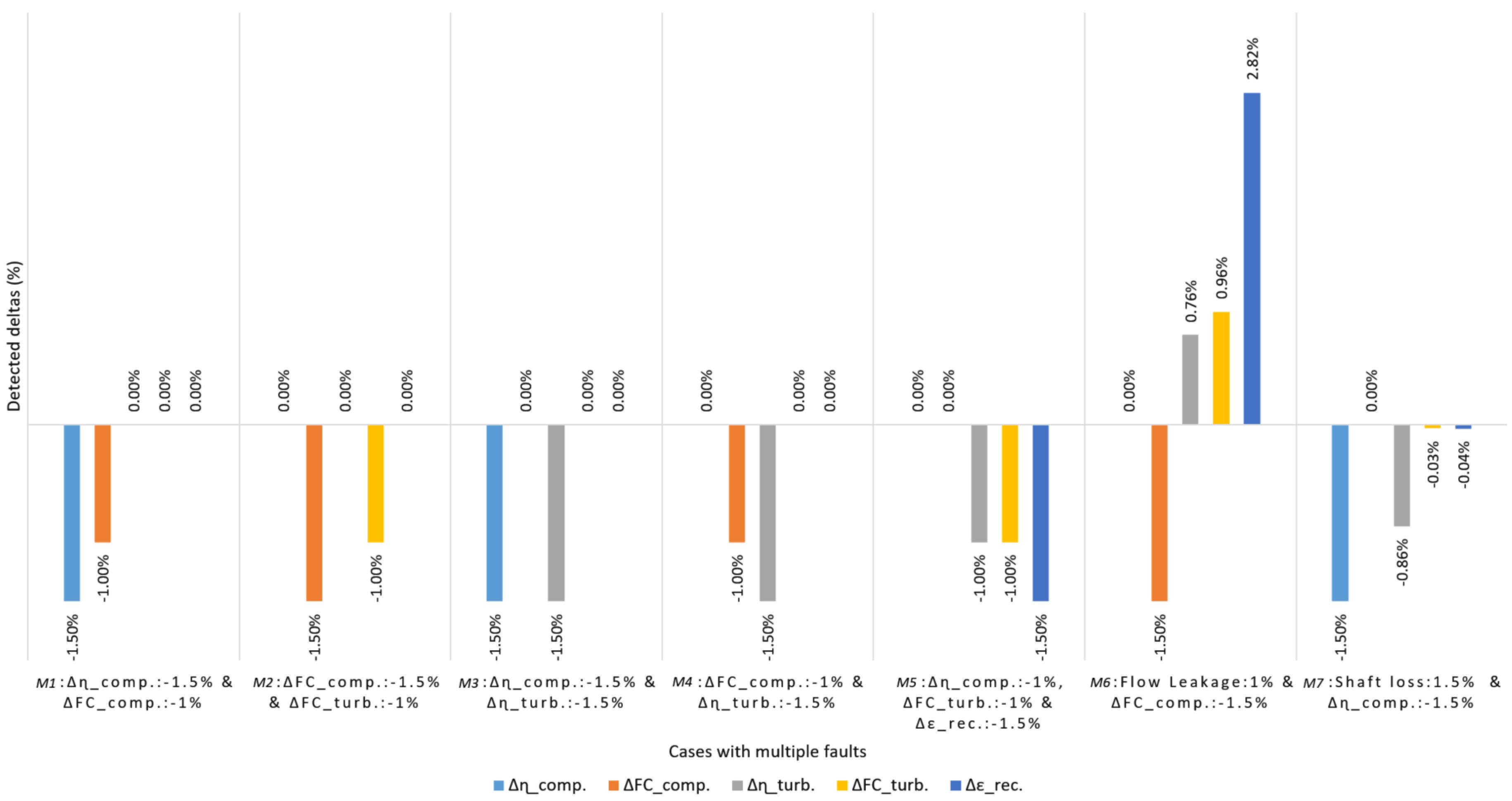
The second set of case studies ($M1$ to $M7$) that includes multiple faults are listed in

Table 7. List of case studies for multiple fault.

Case Identifier	Fault Number	Fault Location and Magnitude
$M1$	Fault-1:	$\Delta {\eta }_{comp.}$ = −1.5%
	Fault-2:	$\Delta F{C}_{comp.}$ = −1.0%
$M2$	Fault-1:	$\Delta F{C}_{comp.}$ = −1.5%
	Fault-2:	$\Delta F{C}_{turb.}$ = −1.0%
$M3$	Fault-1:	$\Delta {\eta }_{comp.}$ = −1.5%
	Fault-2:	$\Delta {\eta }_{turb.}$ = −1.5%
$M4$	Fault-1:	$\Delta F{C}_{comp.}$ = −1.0%
	Fault-2:	$\Delta {\eta }_{turb.}$ = −1.5%
$M5$	Fault-1:	$\Delta {\eta }_{comp.}$ = −1.0%
	Fault-2:	$\Delta F{C}_{comp.}$ = −1.0%
	Fault-3:	$\Delta {ϵ}_{rec.}$ = −1.5%
$M6$	Fault-1:	$Flowleakage$ = 1.0%
	Fault-2:	$\Delta F{C}_{comp.}$ = −1.5%
$M7$	Fault-1:	$Shaftloss$ = 1.5%
	Fault-2:	$\Delta {\eta }_{comp.}$ = −1.5%

. The magnitudes of the faults are chosen between 1% and 1.5% so that the combination is different from the signature database where all the faults are 1% in magnitude.

Results from the AnSyn for simultaneously occurring multiple faults are displayed in Figure 6. As expected, AnSyn can identify correct fault locations and magnitudes for all cases except those including flow leakage and shaft loss. However, when these faults are combined with compressor’s faults, corresponding compressors deltas can be correctly identified by the AnSyn.

The correlation coefficients between exchange rates and signatures for the above cases are reported in

Table 8. Correlation coefficients for cases with multiple faults.

Cases	Correlation between Exchange Rates and Signatures for Cases with Multiple Faults
	$$\begin{gathered} -1\%\Delta {\mathit{\eta }}_{\mathit{comp}.}\& \\ -1\%\Delta {\mathit{FC}}_{\mathit{comp}.} \end{gathered}$$	$$\begin{gathered} -1\%\Delta {\mathit{FC}}_{\mathit{comp}.}\& \\ -1\%\Delta {\mathit{FC}}_{\mathit{turb}.} \end{gathered}$$	$$\begin{gathered} -1\%\Delta {\mathit{\eta }}_{\mathit{comp}.}\& \\ -1\%\Delta {\mathit{\eta }}_{\mathit{turb}.} \end{gathered}$$	$$\begin{gathered} -1\%\Delta {\mathit{FC}}_{\mathit{comp}.}\& \\ -\mathbf{1}\%\Delta {\mathit{\eta }}_{\mathit{turb}.} \end{gathered}$$	$$\begin{gathered} -\mathbf{1}\%\Delta {\mathit{\eta }}_{\mathit{comp}.}, \\ -\mathbf{1}\%\Delta {\mathit{FC}}_{\mathit{turb}.}\& \\ -\mathbf{1}\%\Delta {\mathit{ϵ}}_{\mathit{rec}.} \end{gathered}$$	$$\begin{gathered} \mathbf{1}\%\mathit{Leakage}\& \\ -\mathbf{1}\%\Delta {\mathit{FC}}_{\mathit{comp}.} \end{gathered}$$	$$\begin{gathered} \mathbf{1}\%\mathit{Shaft}\mathit{Loss}\& \\ -\mathbf{1}\%\Delta {\mathit{\eta }}_{\mathit{comp}.} \end{gathered}$$
$M1$	0.997	0.658	0.946	0.871	0.877	0.437	0.971
$M2$	0.745	0.991	0.606	0.617	0.935	−0.093	0.629
$M3$	0.952	0.522	1.000	0.970	0.832	0.653	0.995
$M4$	0.890	0.500	0.972	0.999	0.810	0.722	0.946
$M5$	0.827	0.961	0.723	0.705	0.983	0.002	0.748
$M6$	0.562	−0.071	0.737	0.800	0.315	0.988	0.682
$M7$	0.972	0.553	0.995	0.944	0.846	0.595	1.000

. For each case, this step gives maximum correlation for corresponding signatures from the database that reveals the location of the faults correctly.

Table 9. Fault magnitudes for cases with multiple faults.

Cases	Fault Number	Fault Magnitude	Detected Fault Magnitude Using
			AnSyn	Regression
$\mathit{M}1$	Fault-1:	−1.500	−1.500	−1.486
	Fault-2:	−1.000	−1.000	−0.973
$M2$	Fault-1:	−1.500	−1.500	−1.262
	Fault-2:	−1.000	−1.000	−0.958
$M3$	Fault-1:	−1.500	−1.500	−1.520
	Fault-2:	−1.500	−1.500	−1.522
$M4$	Fault-1:	−1.000	−1.000	−0.948
	Fault-2:	−1.500	−1.500	−1.505
$M5$	Fault-1:	−1.000	−1.000	−0.984
	Fault-2:	−1.000	−1.000	−1.002
	Fault-3:	−1.500	−1.500	−0.993
$M6$	Fault-1:	1.000	-	0.999
	Fault-2:	−1.500	−1.500	−1.527
$M7$	Fault-1:	1.500	-	1.525
	Fault-2:	−1.500	−1.500	−1.517

summarizes the estimated magnitudes of faults for different cases with multiple faults by regression analysis and the comparison with AnSyn. As can be seen, the regression can give good indication of faults magnitude with some level of error, but the AnSyn performs better. The accuracy can be further improved by including more measurements in the multiple linear regression. However, a limited number of measurements are available in reality for such analysis. Additionally, if a sensor fault occurs and one or more measurements need to be removed from the scheme, the accuracy of the regression can even deteriorate. Sensor faults will also reduce the fault detectability by the AnSyn, since corresponding performance delta for the removed measurement also need to be removed from the matching scheme, as presented in Table 2.

Overall, the results presented until now show that the proposed diagnostics scheme can be used to detect the location and magnitude of different component faults with acceptable accuracy. Combining results from AnSyn with the signature-based algorithm increases the confidence on the final outcome of the proposed scheme. However, the above analysis thus far does not include any measurement uncertainty (i.e., sensor noise and bias), which can be quite common in reality. Hence, the influence of measurement uncertainty on the proposed fault diagnostics scheme is assessed in the following section.

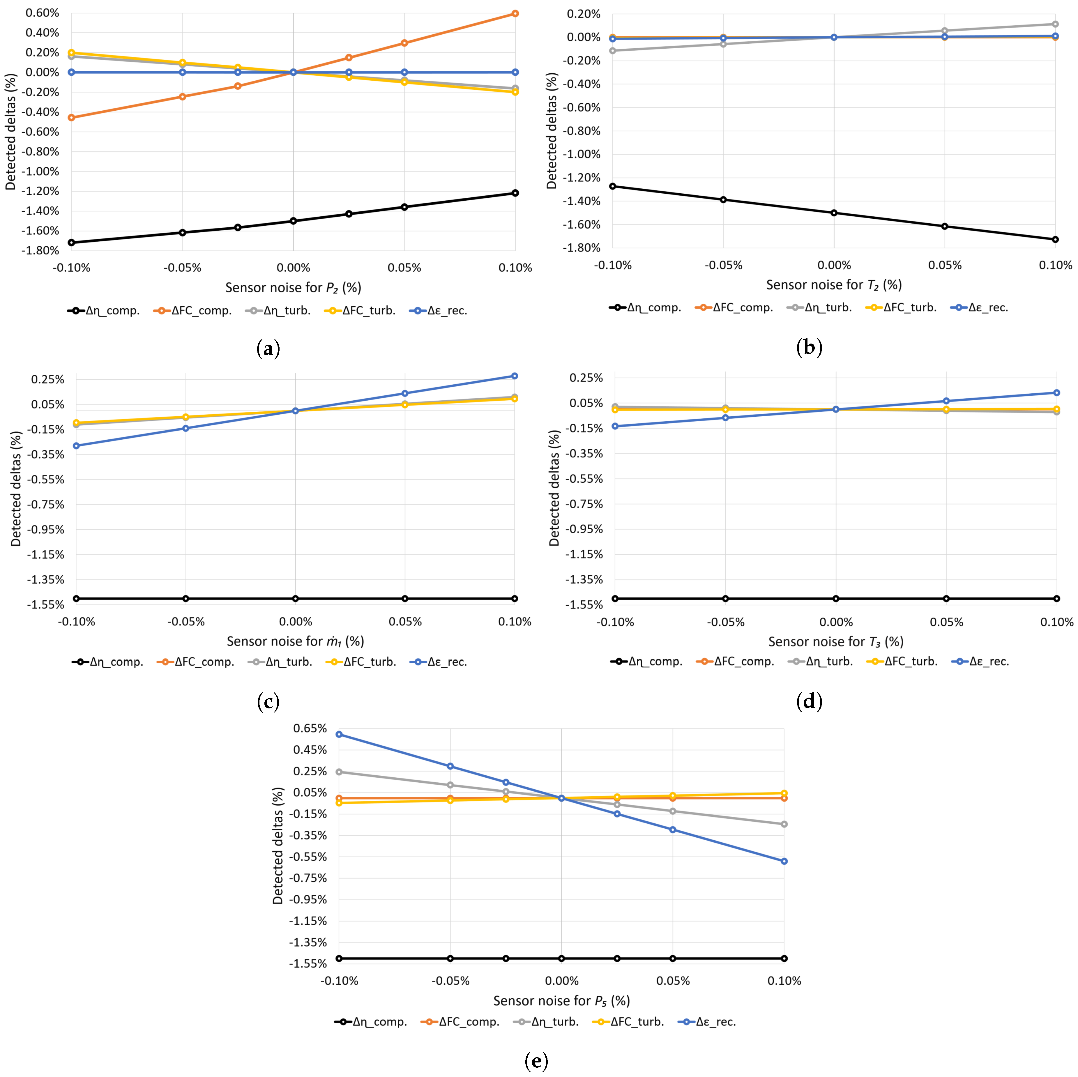
First, the influence of measurement uncertainty on the AnSyn is examined by performing a sensitivity analysis. Here, the measurements corresponding to each of the performance deltas, as listed in Table 2, are varied within measurement uncertainty range. The measurement uncertainties used in this paper are obtained from the literature [42,43]. It is considered here that $P5$ measurement is available through a differential pressure sensor across recuperator.

Figure 7 shows sensitivity analysis of measurement uncertainties on all five performance deltas. Here, case study $"S1"$ i.e., 1.5% drop in compressor isentropic efficiency is considered for this analysis. As can be seen in Figure 7, the compressor isentropic efficiency is only affected by $P_2$ and $T_2$ measurements. However, there is very strong linkage between $P_2$ and compressor flow capacity, and $P_5$ and recuperator effectiveness. Hence, measurement uncertainties in $P_2$ and $P_5$ can give misleading indication of faults related to compressor flow capacity and recuperator effectiveness, respectively; although their magnitudes are not as prominent as the fault. Other measurement uncertainties have negligible influence on different performance deltas. Therefore, it can be summarized from the sensitivity analysis that the influence of measurement uncertainties is limited and will have the effect of a reduced accuracy in fault magnitude estimation. Moreover, the sensor data can be filtered before using it for diagnostics purpose to decrease false alarm due to sensor noise related uncertainties.

Thereafter, the effect of measurement uncertainties on the correlation step is assessed. As in the previous section, the case study $"S1"$, i.e., 1.5% drop in compressor isentropic efficiency is considered. For each of the sensors, maximum deviation in the measurement is assumed. As can be seen in

Table 10. Correlation coefficients for different measurement uncertainties.

Cases	Correlation between Exchange Rates and Signatures for Different Measurement Uncertainties
	$-1\%\Delta {\mathit{\eta }}_{\mathit{comp}.}$	$-1\%\Delta {\mathit{FC}}_{\mathit{comp}.}$	$-1\%\Delta {\mathit{\eta }}_{\mathit{turb}.}$	$-1\%\Delta {\mathit{FC}}_{\mathit{turb}.}$	$-1\%\Delta {\mathit{ϵ}}_{\mathit{rec}.}$
$P_2$–0.1%	0.996	0.692	0.776	0.447	−0.750
$T_2$–0.2%	0.983	0.780	0.885	0.453	−0.860
${\dot{m}}_1$–0.2%	0.989	0.738	0.767	0.615	−0.722
$T_3$–0.2%	0.989	0.620	0.686	0.541	−0.650
$P_5$–0.01%	1.000	0.689	0.784	0.493	−0.754

, the measurement uncertainties has influence on the correlation coefficient. However, the influence is negligible and still faults are identified correctly by giving maximum correlation coefficient for corresponding fault location.

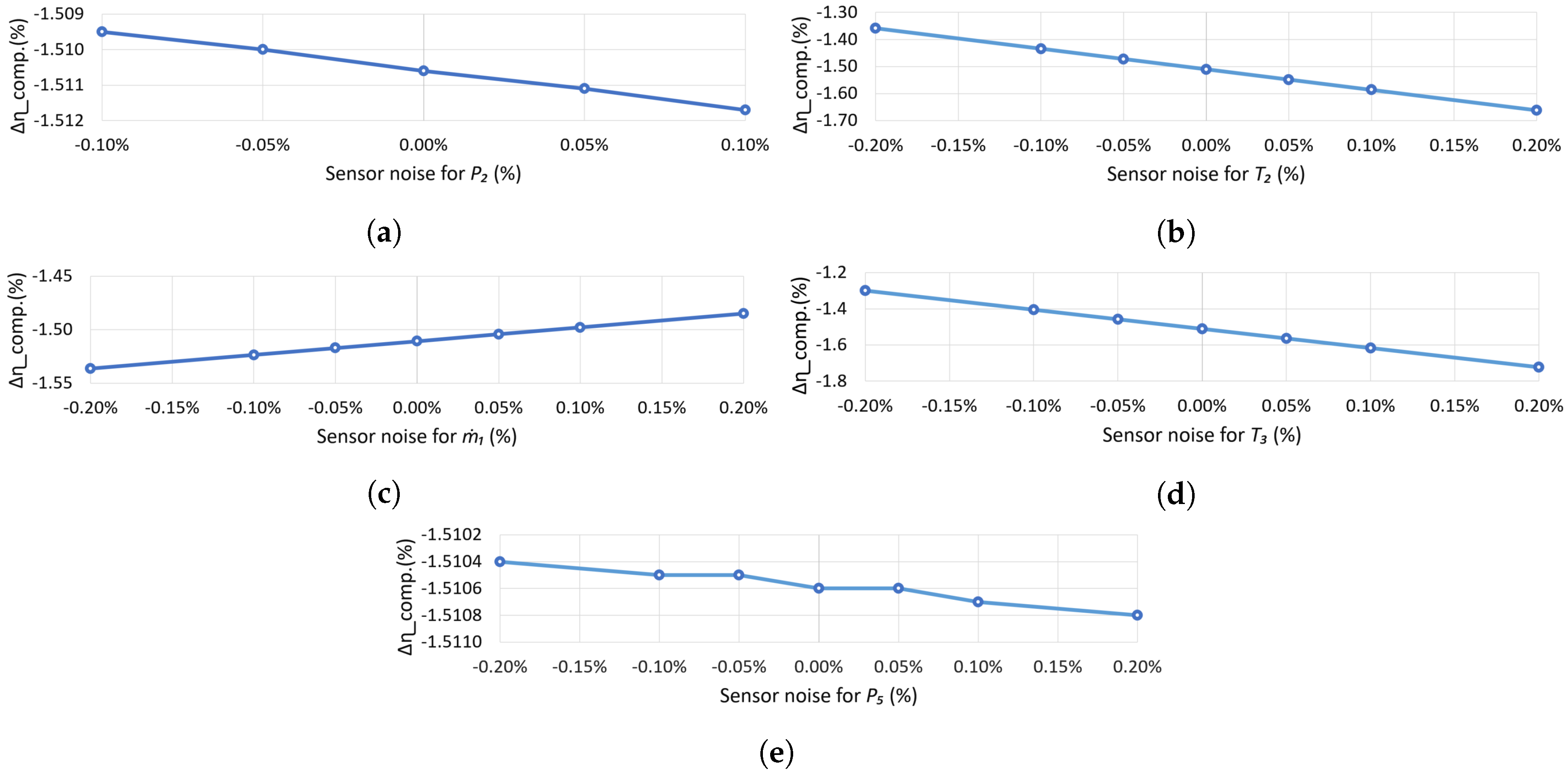
Eventually, the influence of measurement uncertainties on the fault magnitude detection by using linear regression is examined with the help of sensitivity analysis. The sensor measurements are varied by introducing different level of uncertainties and the corresponding fault magnitudes are calculated for case study $S1$. The result of the analysis is summarized in Figure 8. The most influencing measurement uncertainty in this case corresponds to $T_2$ and $T_3$. Despite the high sensitivity for some measurements, the regression can still provide fault magnitude with acceptable accuracy.

5. Conclusions

In this article, a multi-layer approach for monitoring and diagnostics of MGT fleet is investigated. A diagnostics-oriented model based on gas path analysis lies at the core of this approach. Subsequently, a model tuning approach is proposed to account for engine to engine variation as a result of production scatter. The two layers of diagnostics approach that are investigated in this paper include: (1) analysis by synthesis (AnSyn); and (2) signature based algorithm to detect the location and magnitude of different component faults. To perform AnSyn, performance deltas corresponding to each component fault are introduced in the physics-based model, where each delta is associated with a measurement of the engine. The performance deltas are then calculated by using real-time measurements from the engine that gives both location and magnitude of the fault. Due to the lack of measurements, not all the faults can be included in the AnSyn step. Moreover, to improve the robustness of the diagnostics approach, a signature based algorithm is applied as the second layer. Fault signatures were generated with the engine model and compared with the simulated faulty engine data. Correlation function and linear regression are applied to get the location and magnitude of the faults, respectively. Finally, results from both layers are merged together. The proposed diagnostics scheme was tested by formulating case studies corresponding to single and multiple faults. Furthermore, sensitivity studies were performed for different measurement uncertainties (i.e., sensor noise and bias) to evaluate the robustness of the scheme against measurement uncertainties. The result shows that the proposed diagnostics approach performs satisfactorily even under measurement uncertainties. Overall, magnitude of triple faults seems hard to detect by signature based algorithm, given that the number of measurements available for the analysis is limited to five. The accuracy can be improved by including more measurements in the analysis. In case of sensor faults, the corresponding measurements need to be removed from the matching scheme for AnSyn along with their associated performance deltas. This will unavoidably reduce the detectability of the corresponding fault by AnSyn. At the same time, the signature based algorithm might result in reduced accuracy or false alarm.

References

- Zampilli, M.; Bidini, G.; Laranci, P.; D’Amico, M.; Bartocci, P.; Fantozzi, F. Biomass microturbine based EFGT and IPRP cycles: Environmental impact analysis and comparison. In Proceedings of the Asme Turbo Expo: Turbine Technical Conference and Exposition, Charlotte, NC, USA, 26–30 June 2017; Volume 3, pp. 1–9. [Google Scholar] [CrossRef]
- European Turbine Network (ETN). R & D Recommendation Report 2016—For the Next Generation of Gas Turbines; Technical Report; European Turbine Network (ETN): Brussels, Belgium, 2017. [Google Scholar]
- Owens, B. The Rise of Distributed Power; Technical Report; General Electric Company: Boston, MA, USA, 2014. [Google Scholar] [CrossRef]
- European Parliament. EU Startegy on Heating and Cooling; 2016/2058(INI); European Parliament: Brussels, Belgium, 2016. [Google Scholar]
- European Turbine Network (ETN). Micro Gas Turbine Technology Summary: Research and Development for European Collaboration; Technical Report; European Turbine Network (ETN): Brussels, Belgium, 2017. [Google Scholar]
- Gopisetty, S.; Treffinger, P. Generic Combined Heat and Power (CHP) Model for the Concept Phase of Energy Planning Process. Energies 2016, 10, 11. [Google Scholar] [CrossRef]
- Rahman, M.; Malmquist, A. Modeling and Simulation of an Externally Fired Micro-Gas Turbine for Standalone Polygeneration Application. J. Eng. Gas Turbines Power 2016, 138, 112301. [Google Scholar] [CrossRef]
- Kim, S.; Chun Kim, K. Performance Analysis of Biogas-Fueled SOFC/MGT Hybrid Power System in Busan, Republic of Korea. Proceedings 2018, 2, 605. [Google Scholar] [CrossRef]
- Kalathakis, C.; Aretakis, N.; Mathioudakis, K. Solar Hybrid Micro Gas Turbine Based on Turbocharger. Appl. Syst. Innov. 2018, 1, 27. [Google Scholar] [CrossRef]
- Kyprianidis, K.G.; Quintero, R.F.C.; Pascovici, D.S.; Ogaji, S.O.T.; Pilidis, P.; Kalfas, A.I. EVA: A Tool for EnVironmental Assessment of Novel Propulsion Cycles. In Proceedings of the ASME Turbo Expo 2008: Power for Land, Sea, and Air, Berlin, Germany, 9–13 June 2008; pp. 547–556. [Google Scholar]
- Kyprianidis, K.G.; Dahlquist, E. On the trade-off between aviation NOx and energy efficiency. Appl. Energy 2017, 185, 1506–1516. [Google Scholar] [CrossRef]
- Razak, A.M.Y. Industrial Gas Turbines: Peformance and Operability; Woodhead Publishing Limited, Abington Hall: Abington, UK, 2007; p. 9. [Google Scholar]
- Kurz, R.; Brun, K.; Wollie, M. Degradation effects on industrial gas turbines. J. Eng. Gas Turbines Power 2009, 131, 62401. [Google Scholar] [CrossRef]
- Kurz, R. Gas Turbine Degradation. In Proceedings of the 43rd Turbomachinery & 30th Pump Users Symposia, Houston, TX, USA, 23–25 September 2014; pp. 1–36. [Google Scholar]
- Tahan, M.; Tsoutsanis, E.; Muhammad, M.; Abdul Karim, Z.A. Performance-based health monitoring, diagnostics and prognostics for condition-based maintenance of gas turbines: A review. Appl. Energy 2017, 198, 122–144. [Google Scholar] [CrossRef] [Green Version]
- Li, Y.G. Performance-analysis-based gas turbine diagnostics: A review. Proc. Inst. Mech. Eng. Part A J. Power Energy 2002, 216, 363–377. [Google Scholar] [CrossRef] [Green Version]
- Volponi, A.J.; Doel, D.L.; Provost, M.J.; Grodent, M.; Navez, A.; Mathioudakis, K.; Romessis, C.; Stamatis, A.; Singh, R. Gas Turbine Condition Monitoring and Fault Diagnostics; Lecture Series 2003-1; Von Karman Institute for Fluid Dynamics: Brussels, Belgium, 2003. [Google Scholar]
- Marinai, L.; Probert, D.; Singh, R. Prospects for aero gas-turbine diagnostics: A review. Appl. Energy 2004, 79, 109–126. [Google Scholar] [CrossRef]
- Stamatis, A.G. Evaluation of gas path analysis methods for gas turbine diagnosis. J. Mech. Sci. Technol. 2011, 25, 469–477. [Google Scholar] [CrossRef]
- Fentaye, A.D.; Gilani, S.I.U.H.; Baheta, A.T. Gas turbine gas path diagnostics: A review. In Proceedings of the 3rd International Conference on Mechanical Engineering Research (ICMER 2015), Kuantan, Malaysia, 18–19 August 2015; Volume 74, p. 5. [Google Scholar]
- Urban, L.A. Gas Turbine Engine Parameter Interrelationships, 1st ed.; Hamilton Standard Division of United Aircraft Corporation: Windsor Locks, CT, USA, 1967. [Google Scholar]
- Urban, L.A. Parameter Selection for Multiple Fault Diagnostics of Gas Turbine Engines. J. Eng. Power 1975, 97, 225–230. [Google Scholar] [CrossRef]
- Urban, L.A.; Volponi, A.J. Mathematical Methods of Relative Engine Performance Diagnostics; Technical Paper; Society of Automotive Engineers (SAE): Warrendale, PA, USA, 1992. [Google Scholar] [CrossRef]
- Passalacque, J. Description of automatic gas turbine engine trends diagnostic system. In Proceedings of the 1st National Research Council of Canada (NRCC) Conference on Gas Turbines Operations and Maintenance, Ottawa, ON, Canada, 1974. [Google Scholar]
- Stamatis, A.; Mathioudakis, K.; Papailiou, K.; Berios, G. Jet engine fault detection with discrete operating points gas path analysis. J. Propuls. Power 1991, 7, 1043–1048. [Google Scholar] [CrossRef]
- Simani, S.; Patton, R.J.; Daley, S.; Pike, A. Identification and fault diagnosis of an industrial gas turbine prototype model. In Proceedings of the 39th IEEE Conference on Decision and Control, Sydney, Australia, 12–15 December 2000; Volume 3, pp. 2615–2620. [Google Scholar]
- House, P. Gas Path Analysis Techniques Applied to a Turboshaft Engine. Ph.D. Thesis, Cranfield University, Cranfield, Bedfordshire, UK, 1992. [Google Scholar]
- Esher, P.C. Pythia: An Object-Oriented Gas Path Analysis Computer Program for General Applications. Ph.D. Thesis, Cranfield University, Cranfield, UK, 1995. [Google Scholar]
- Stamatis, A.; Mathioudakis, K.; Papailiou, K.D. Adaptive Simulation of Gas Turbine Performance. J. Eng. Gas Turbines Power 1990, 112, 168–175. [Google Scholar] [CrossRef]
- Li, Y.G. Gas Turbine Performance and Health Status Estimation Using Adaptive Gas Path Analysis. J. Eng. Gas Turbines Power 2010, 132, 41701–41709. [Google Scholar] [CrossRef]
- Larsson, E.; Åslund, J.; Frisk, E.; Eriksson, L. Gas Turbine Modeling for Diagnosis and Control. J. Eng. Gas Turbines Power 2014, 136, 71601–71617. [Google Scholar] [CrossRef]
- Liu, Y. Design of Fault Detection System for a Heavy Duty Gas Turbine with State Observer and Tracking Filter. In Proceedings of the ASME Turbo Expo 2017: Turbomachinery Technical Conference and Exposition, Charlotte, NC, USA, 26–30 June 2017; p. V006T05A017. [Google Scholar]
- Kang, D.W.; Kim, T.S. Model-based performance diagnostics of heavy-duty gas turbines using compressor map adaptation. Appl. Energy 2018, 212, 1345–1359. [Google Scholar] [CrossRef]
- Koskoletos, O.A.; Aretakis, N.; Alexiou, A.; Romesis, C.; Mathioudakis, K. Evaluation of Aircraft Engine Diagnostic Methods through ProDiMES. In Proceedings of the ASME Turbo Expo 2018: Turbomachinery Technical Conference and Exposition, Oslo, Norway, 11–15 June 2018; p. V006T05A023. [Google Scholar]
- Davison, C.R.; Birk, A.M. Automated fault diagnosis of a micro turbine with comparison to a neural network technique. In Proceedings of the ASME Turbo Expo 2006: Power for Land, Sea, and Air, Barcelona, Spain, 8–11 May 2006; pp. 795–804. [Google Scholar]
- Davison, C.R.; Birk, A.M. Prediction of time until failure for a micro turbine with unspecified faults. In Proceedings of the ASME Turbo Expo 2006: Power for Land, Sea, and Air, Barcelona, Spain, 8–11 May 2006; pp. 805–814. [Google Scholar]
- Mahmood, M.; Martini, A.; Traverso, A.; Bianchi, E. Model Based Diagnostics of AE-T100 Micro Gas Turbine. In Proceedings of the ASME Turbo Expo 2016: Turbomachinery Technical Conference and Exposition, Seoul, Korea, 13–17 June 2016; p. V006T05A021. [Google Scholar]
- Kim, M.J.; Kim, J.H.; Kim, T.S. The effects of internal leakage on the performance of a micro gas turbine. Appl. Energy 2018, 212, 175–184. [Google Scholar] [CrossRef]
- Zaccaria, V.; Stenfelt, M.; Aslanidou, I.; Kyprianidis, K.G. Fleet Monitoring and Diagnostics Framework Based on Digital Twin of Aero-Engines. In Proceedings of the ASME Turbo Expo 2018: Turbomachinery Technical Conference and Exposition, Oslo, Norway, 11–15 June 2018; p. V006T05A021. [Google Scholar]
- Ogaji, S.O.T.O. Advanced Gas-Path Fault Diagnostics for Stationary Gas Turbines. Ph.D. Thesis, Cranfield University, Cranfield, UK, 2003. [Google Scholar]
- Aslanidou, I.; Zaccaria, V.; Rahman, M.; Oostveen, M.; Olsson, T.; Kyprianidis, K.G. Towards an Integrated Approach for Micro Gas Turbine Fleet Monitoring, Control, and Diagnostics. In Proceedings of the Global Power and Propulsion Society (GPPS) Forum 2018, Zurich, Switzerland, 10–22 January 2018. [Google Scholar]
- Badami, M.; Giovanni Ferrero, M.; Portoraro, A. Dynamic parsimonious model and experimental validation of a gas microturbine at part-load conditions. Appl. Therm. Eng. 2015, 75, 14–23. [Google Scholar] [CrossRef]
- Mohtar, H.; Chesse, P.; Chalet, D. Describing uncertainties encountered during laboratory turbocharger compressor tests. Exp. Tech. 2012, 36, 53–61. [Google Scholar] [CrossRef]
Figure 1.
Layout of the MGT in CHP configuration (MGT: Micro Gas Turbine; CHP: Combined Heat and Power).
Figure 2.
Scheme for model tuning.
Figure 3.
Scheme for fault identification (ISA: International Standard Atmosphere).
Figure 4.
Comparison between model and performance test results for off-design operation (PWX: shaft power).
Figure 5.
Fault location and severity for cases with single faults detected by AnSyn (AnSyn: analysis by synthesis).
Figure 6.
Preliminary estimation of fault location and severity for cases with multiple faults by AnSyn.
Figure 7.
Sensitivity of AnSyn against measurement uncertainties in: (a) ; (b) ; (c) ; (d) ; and (e) .
Figure 8.
Sensitivity of fault magnitude detection using linear regression against different measurement uncertainties in: (a) ; (b) ; (c) ; (d) ; and (e) .