A Novel Framework for Parameter and State Estimation of Multicellular Systems Using Gaussian Mixture Approximations

Abstract

Multicellular systems play an important role in many biotechnological processes. Typically, these exhibit cell-to-cell variability, which has to be monitored closely for process control and optimization. However, some properties may not be measurable due to technical and financial restrictions. To improve the monitoring, model-based online estimators can be designed for their reconstruction. The multicellular dynamics is accounted for in the framework of population balance models (PBMs). These models are based on single cell kinetics, and each cellular state translates directly into an additional dimension of the obtained partial differential equations. As multicellular dynamics often require detailed single cell models and feature a high number of cellular components, the resulting population balance equations are often high-dimensional. Therefore, established state estimation concepts for PBMs based on discrete grids are not recommended due to the large computational effort. In this contribution a novel approach is proposed, which is based on the approximation of the underlying number density functions as the weighted sum of Gaussian distributions. Thus, the distribution is described by the characteristic properties of the individual Gaussians, like the mean and covariance. Thereby, the complex infinite dimensional estimation problem can be reduced to a finite dimension. The characteristic properties are estimated in a recursive approach. The method is evaluated for two academic benchmark examples, and the results indicate its potential for model-based online reconstruction for multicellular systems.

1. Introduction

Multicellular systems are not only found at the core of many fundamental biomedical processes like cell differentiation [1] and wound healing, but also play an essential role in a wide spectrum of biotechnological processes ranging from pharmaceutical manufacturing [2,3] to biopolymer production [4] to biological waste-water treatment [5]. The individual cells do not only interact with each other, but also with their environment. These interactions are affected by individual cellular properties like cell volume and gene/protein expression levels, which underlie a certain cell-to-cell variability, i.e., the properties appear distributed within the cell population. The reasons for such heterogeneities are manifold, including differences in local substrate concentrations [6] or non-synchronous cell-cycles [7], as well as stochastic effects on the genomic and proteomic level [8]. From an evolutionary point of view, this variability is argued to benefit the robustness of the cell population against rapid environmental changes. However, on an industrial scale, such variabilities can have undesired effects like decreased product yields and even result in an unstable behavior [9]. Therefore, close monitoring of the cellular properties and their distribution within the population is of paramount importance. In the last few decades, sophisticated measurement techniques such as flow and mass cytometry have been developed that allow inferring the distributions of cellular properties [10]. Nevertheless, these only supply information on representative samples from the cell population at discrete time points, so-called “snapshot data” [11]. Moreover, due to technical limitations (no established staining procedure), financial considerations (expensive dyes) or safety restrictions (hazardous staining procedures), only a limited amount of information is available on at least some of the cellular properties. A descriptive example is depicted in Figure 1: Cells are characterized by individual cell size and growth rate. Though individual growth rate can be accessed via sophisticated experiments in principle [12], measurement of individual cell size is much easier and less expensive. Assuming that exclusively the latter is measured, instead of a two-dimensional distribution over both variables, only a one-dimensional number distribution over the cell size is obtained from flow cytometric analysis.

For reconstructing unmeasured cellular characteristics, model-based state estimation techniques can be applied (see Figure 1 for a schematic representation): A mathematical model of the process is run in parallel to the process itself. The model is updated online with available measurements, and the model variables are used as surrogates for the real process variables. Such state estimation techniques, e.g., Luenberger observers and Kalman filters, are well studied and widely applied for systems with dynamics described by ordinary differential equations (ODEs) (see, e.g., [13]). Modeling of multicellular systems, as done in the population balance modeling framework [14], results in rather complex expressions: Generally, multi-dimensional population balance equations (PBEs) describing the dynamics of the cell number density function (NDF) are obtained. As these represent multi-dimensional partial-integro differential equations, established state estimation methods are not applicable directly. A grid-based discretization approach as presented for one-dimensional PBEs characterizing particle formation processes (see, e.g., [15]) is not recommended, as the computational effort becomes unreasonably large in the multi-dimensional case.

This motivates the design of a novel state estimation concept for PBEs proposed in this manuscript. The basic idea can be summarized as follows: The full NDF is approximated by a Gaussian mixture distribution (GMD) [16]. This technique is already established for the statistical analysis of heterogeneous cell populations measured with appropriate techniques such as flow and mass cytometry (see, e.g., [17,18] and the references therein). Instead of accounting for the dynamics of the full NDF, one only describes the dynamics of integral quantities of the Gaussians. In contrast to [19], we not only characterize those dynamics in terms of the Gaussians’ means alone, but also account for the dynamics of the Gaussians’ covariances. Subsequently, estimators are applied to reconstruct means and (co)variances of these Gaussian distributions. Thereby, the approach guarantees high flexibility, as it is not limited to a specific numerical solution method like the above-mentioned discretization-based approach: Depending on the problem, tailored numerical schemes can be implemented to compute the integral quantities of the Gaussians, e.g., moment methods [20]. Moreover, one is not restricted to a specific type of estimator: in principle, any established state estimation or observer design technique is applicable.

This manuscript is structured as follows: At first, the modeling of multicellular systems dynamics using PBEs is briefly introduced. Subsequently, it is explained how the full NDF is approximated with GMDs and how the dynamics of their integral quantities can be derived from the corresponding PBEs. The next section outlines the application of Kalman and particle filters, both representing established estimation techniques [13], for reconstructing the integral properties of the Gaussian distributions in special cases. Results for two numerical case studies are shown and discussed. A summary is given and potential future work outlined.

2. Materials and Methods

2.1. Modeling of the Multicellular Dynamics

Each cell can be characterized by individual properties, like size/shape or (bio)chemical composition, which are summarized in the cellular state vector $\mathbf{z}={\left[z_1,\dots ,z_{N_z}\right]}^T$. For single cell modeling of their dynamics, complex cellular mechanics on different time and size scales, such as metabolic, proteomic, genomic and regulatoric, have to be taken into account. In the following, it is assumed that the temporal evolution of $\mathbf{z}$ can be sufficiently described with a system of stochastic differential equations (SDEs) [21]:

$$\begin{array}{c}\hfill \mathrm{d}\mathbf{z}\left(t\right)={\mathbf{f}}_z(\mathbf{z}\left(t\right),t)\mathrm{d}t+\sqrt{2}D(\mathbf{z}\left(t\right),t)\mathrm{d}{W}_t.\end{array}$$

(1)

Therein, the vector field ${\mathbf{f}}_z={\left[f_{z_1},\dots ,f_{z_{N_z}}\right]}^T$ characterizes deterministic mechanics, while the remainder of the right-hand side accounts for stochastic effects by a vector Wiener-process $W_t$ in the space of the intracellular coordinates. Here, $D\left(\mathbf{z}\right(t),t)$ is a square matrix of dimension $N_z$ characterizing the effects of the Wiener-process on the cellular dynamics. Its elements may depend on $\mathbf{z}\left(t\right)$ and extracellular components. In the case of negligible stochasticity, Equation (1) reduces to a set of ordinary differential equations (ODEs):

$$\begin{array}{c}\hfill \dot{\mathbf{z}}\left(t\right)={\mathbf{f}}_z(\mathbf{z}\left(t\right),t).\end{array}$$

(2)

As already pointed out in the Introduction, several reasons may put restrictions on the available measurements such that only certain cellular properties or functions thereof are accessible, which is modeled by the output equation:

$$\begin{array}{c}\hfill {\mathbf{y}}_z\left(t\right)={\mathbf{h}}_z(\mathbf{z}\left(t\right),t)=\left[y_{z_1}\left(t\right),\dots ,y_{z_{N_y}}\left(t\right)\right].\end{array}$$

(3)

In a population of cells, individual properties underlie cell-to-cell variability and thus appear distributed. Dynamics of the distributed properties in terms of the cell number density distribution $n(t,\mathbf{z})$ can be described in the framework of population balance modeling (PBM), giving rise to the general population balance equation [21]:

$$\begin{array}{c}\hfill \frac{\partial n(t,\mathbf{z})}{\partial t}=-{\nabla }_{\mathbf{z}}·{\mathbf{f}}_z(\mathbf{z},t)n(t,\mathbf{z})+{\nabla }_{\mathbf{z}}{\nabla }_{\mathbf{z}}:\tilde{D}(\mathbf{z}\left(t\right),t)n(t,\mathbf{z})+P(n(t,\mathbf{z}),\mathbf{z}\left(t\right),t)\end{array}$$

(4)

where:

$$\begin{array}{c}\hfill \tilde{D}(\mathbf{z}\left(t\right),t)=D_z(\mathbf{z}\left(t\right),t)D_z^T(\mathbf{z}\left(t\right),t)\end{array}$$

(5)

and the double dot inner product is defined as:

$$\begin{array}{c}\hfill {\nabla }_{\mathbf{z}}{\nabla }_{\mathbf{z}}:\tilde{D}(\mathbf{z}\left(t\right),t)n(t,\mathbf{z})=\sum _{i=1}^{N_z}\sum _{i=1}^{N_z}\frac{{\partial }^2}{\partial z_i\partial z_j}\left\{{\tilde{D}}_{i,j}(\mathbf{z}\left(t\right),t)n(t,\mathbf{z})\right\}.\end{array}$$

(6)

Therein, ${\tilde{D}}_{i,j}(\mathbf{z}\left(t\right),t)$ denotes the $(i,j)$-element of $\tilde{D}(\mathbf{z}\left(t\right),t)$. Alternatively, Equation (4) can thus be written as:

$$\begin{array}{c}\hfill \frac{\partial n(t,\mathbf{z})}{\partial t}=-\sum _{i=1}^{N_z}\frac{\partial }{\partial z_i}\left\{f_{z_i}(\mathbf{z}\left(t\right),t)n(t,\mathbf{z})\right\}+\sum _{i=1}^{N_z}\sum _{i=1}^{N_z}\frac{{\partial }^2}{\partial z_i\partial z_j}\left\{{\tilde{D}}_{i,j}(\mathbf{z}\left(t\right),t)n(t,\mathbf{z})\right\}+P(n(t,\mathbf{z}),\mathbf{z}\left(t\right),t).\end{array}$$

(7)

The left-hand sides of Equations (4) and (7) characterize accumulation; while the first terms on the right-hand side describe the change of properties resulting from deterministic cellular kinetics (e.g., growth and biochemical reactions), the second stochastic effects and the third terms contain source processes like cell birth (e.g., budding and division) and death (e.g., apoptosis). In this contribution, rather small time horizons are considered on which the first effect is dominant in comparison to the latter two, such that we take $P\left(n\right(t,\mathbf{z}),\mathbf{z},t)=0$. It has to be mentioned that coupling to other species with distributed parameters (e.g., a second cell population) and non-distributed parameters (e.g., extracellular substrates) has also been neglected in this study. In the case of restrictions on measurements as described earlier, only projections of $n(t,\mathbf{z})$, but not the full NDF itself can be measured:

$$\begin{array}{c}\hfill n_{\mathbf{y}}(t,\mathbf{y})=H(t,n(t,\mathbf{z}),\mathbf{z}).\end{array}$$

(8)

Here, $H(t,n(t,\mathbf{z}),\mathbf{z})$ is the output operator that depends on the available single cell measurements represented by Equation (3). For example, out of two cellular states $\mathbf{z}=\left[z_1,z_2\right]$, only one may be accessible $y_z=z_2$ (e.g., cell size, but not cell growth) via flow cytometry. As a result, only the marginal distribution:

$$\begin{array}{c}\hfill n_y(t,z_2)=H(t,n(t,\mathbf{z}),\mathbf{z})=\underset{z_{1,min}}{\overset{z_{1,max}}{\int }}n(t,\mathbf{z})\mathrm{d}{z}_1\end{array}$$

(9)

will be available.

The main idea of the proposed approach predicates on approximation of the NDF with basis functions, e.g., a sum of Gaussian normal distributions:

$$\begin{array}{c}\hfill n(t,·)\approx \sum _{i=1}^{N_{GMD}}{a}^{\left(i\right)}\left(t\right)·\mathcal{N}({\mu }^{\left(i\right)}\left(t\right),{\Sigma }^{\left(i\right)}\left(t\right),·).\end{array}$$

(10)

It is well known that each distribution can be approximated by such a mixture density, yet a large number of individual Gaussians may be required to obtain a sufficient accuracy of the approximation. Furthermore, it has to be mentioned that there are several approaches to obtain these approximations, each having certain advantages and drawbacks (see, e.g., [16] and the references therein). For the proposed estimation method outlined in the following, the specific method is not important, as long as the approximations are sufficiently accurate. To improve the readability, dependence on t will not be written out explicitly in the following. The dynamics of the full NDF can be characterized by the dynamics of integral quantities of individual elements, i.e., mixture component $a^{\left(i\right)}$ (i.e., the zeroth order moment), vector of mean values ${\mu }^{\left(i\right)}$ (i.e., the normalized first order moments) and covariance ${\Sigma }^{\left(i\right)}$ (consists of normalized central second order moments). The corresponding state vectors for individual densities are given as:

$$\begin{array}{c}\hfill {\mathbf{x}}_{}^{\left(i\right)}=\left[a^{\left(i\right)},{\mu }^{\left(i\right)},{\Sigma }^{\left(i\right)}\right],i=1,\dots ,N_{GMD}.\end{array}$$

(11)

It is obvious that their temporal evolution and the corresponding measurement vector:

$$\begin{array}{cc}\hfill {\dot{\mathbf{x}}}_{}^{\left(i\right)}& ={\mathbf{f}}_{}^{}({\mathbf{x}}_{}^{\left(i\right)},\mathbf{v}),i=1,\dots ,N_{GMD}\hfill \end{array}$$

(12)

$$\begin{array}{cc}\hfill {\mathbf{y}}_{}^{\left(i\right)}& ={\mathbf{h}}_{}({\mathbf{x}}_{}^{\left(i\right)},\mathbf{w}),i=1,\dots ,N_{GMD}\hfill \end{array}$$

(13)

depend directly on the population balance Equation (4) and the available cellular measurement information. For the general nonlinear case, a closed set of equations is only found in rare cases, and thus, one relies on approximate closure techniques. These include power series expansions and approximate moment methods [20]. The variables $\mathbf{v}$ and $\mathbf{w}$ denote random perturbations on the process dynamics and measurements not included in the model formulation. For linear intracellular dynamics:

$$\begin{array}{c}\hfill {\mathbf{f}}_z\left(\mathbf{z}\right)=A_z·\mathbf{z}\end{array}$$

(14)

is obtained. Here, $A_z$ is an $N_z$-dimensional square matrix. If furthermore, the measurement dynamics are linear:

$$\begin{array}{c}\hfill {\mathbf{h}}_z\left(\mathbf{z}\right)=C_z·\mathbf{z}\end{array}$$

(15)

a closed set of equations is found for the dynamics of means and covariances. In case the stochasticity is assumed to be independent from the intracellular properties and time invariant $D(\mathbf{z},t)=D$, the following equations are obtained:

$$\begin{array}{c}\hfill {\dot{\mu }}^{\left(i\right)}=A_z·{\mu }^{\left(i\right)},{\dot{\Sigma }}^{\left(i\right)}=A_z·{\Sigma }^{\left(i\right)}+{\Sigma }^{\left(i\right)}·A_z^T+D.\end{array}$$

(16)

2.2. Observability of Multicellular Systems Dynamics

Prior to the design of any state estimator/observer, it has to be clarified if it is even possible to reconstruct non-measurable quantities from measurable ones with a model-based approach. This issue, also known as observability analysis, has received much attention over the last few decades. Initially, the focus was on finite dimensional systems dynamics described by linear and nonlinear ordinary differential equation systems [22,23]. Additionally, more general graph-based concepts were developed [24,25]. However, the application of these concepts to population balance models is scarce and mostly relies on a prior discretization step that transforms the infinite dimensional system to a high-dimensional system of ODEs (e.g., [26]). Recently, a new concept was presented that allows statements on the observability of ensemble systems [27]. Unfortunately, only sufficient conditions are provided for a limited class of individual (cellular) dynamics, and more general effects like cell death and cell division, as well as interaction with a non-distributed species are neglected.

In the proposed framework, the infinite dimensional system represented by the multi-dimensional PBE in Equation (4) is transformed to a finite dimension using the approximation of the multi-dimensional number density distributions by sums of the Gaussian distribution. This allows a straightforward analysis of observability in multicellular systems dynamics with established methods from linear and nonlinear systems theory. In the case of linear single cell kinetics, the overall dynamic and output equations of individual GMDs are given as:

$$\begin{array}{c}\hfill {\dot{\mathbf{x}}}^{\left(i\right)}=\frac{\mathrm{d}}{\mathrm{d}t}\left(\begin{array}{c}{\mu }^{\left(i\right)}\\ {\tilde{\Sigma }}^{\left(i\right)}\end{array}\right)=A{\mathbf{x}}^{\left(i\right)}+\left(\begin{array}{c}\mathbf{0}\\ \tilde{D}\end{array}\right),{\mathbf{y}}^{\left(i\right)}=C{\mathbf{x}}^{\left(i\right)}.\end{array}$$

(17)

Therein, the vector ${\tilde{\Sigma }}^{\left(i\right)}$ contains all diagonal and upper-diagonal elements of ${\Sigma }^{\left(i\right)}$, and the vector $\tilde{D}$ contains the corresponding values of D. The dynamic system in Equation (17) is observable if the Kalman rank condition [22]:

$$\begin{array}{c}\hfill rank\left(W_0\right)=\mathrm{d}im\left({\mathbf{x}}^{\left(i\right)}\right)=N_{\mathbf{x}},W_0=\left[\begin{array}{c}C\\ C·A\\ ⋮\\ C·A^{N_{\mathbf{x}}-1}\end{array}\right]\end{array}$$

(18)

is fulfilled. For more general nonlinear dynamics represented by Equation (12), weak local observability is given under the following (sufficient) condition [23]:

$$\begin{array}{c}\hfill rank\left(\frac{\partial Q}{\partial {\mathbf{x}}^{\left(i\right)}}\right)=N_{\mathbf{x}},Q=\left(\begin{array}{c}{\mathbf{y}}^{\left(i\right)}\\ \frac{\mathrm{d}{\mathbf{y}}^{\left(i\right)}}{\mathrm{d}t}\\ ⋮\\ \frac{{\mathrm{d}}^{N_{\mathbf{x}}-1}{\mathbf{y}}^{\left(i\right)}}{\mathrm{d}{t}^{N_{\mathbf{x}}-1}}\end{array}\right)=\left[\begin{array}{c}\mathbf{h}\\ {\mathcal{L}}_{\mathbf{f}}{\mathbf{h}}^{\left(i\right)}\\ ⋮\\ {\mathcal{L}}_{\mathbf{f}}^{N_{\mathbf{x}}-1}{\mathbf{h}}^{\left(i\right)}\end{array}\right].\end{array}$$

(19)

Furthermore, the system could also be tested for structural observability [24,26] posing a necessary condition on local observability. It has to be mentioned that these conditions are only valid for individual state vectors ${\dot{\mathbf{x}}}^{\left(i\right)}$, but not for the whole system, i.e., all GMDs $i=1,\dots ,N_{GMD}$ at once. However, it is immediately clear that the previously presented conditions have to be fulfilled for the special case $N_{GMD}=1$. For $N_{GMD}>1$, a data association algorithm is necessary that assigns $N_{GMD}$ model outputs ${\mathbf{y}}^{\left(i\right)}$ to $N_{GMD}$ measurements ${\mathbf{y}}_{meas}^{\left(i\right)}$. Here, in addition to the rank conditions in Equations (18) and (19), simultaneous convergence of the data association algorithm has to be guaranteed. Derivation of a complete set of conditions for the latter is beyond the scope of this contribution and represents a challenge for future research efforts. Possible solution approaches may be found in the field of multiple target tracking (see [28] and the references therein).

2.3. Estimator Design

The second key idea of the approach is to design suitable estimators for the state vectors defined in Equation (11) instead of the full NDF. Depending on the dynamics described in Equation (12), different established concepts may be applied to reconstruct the full state vector $\mathbf{x}$ from the available measurements. As alternative to deterministic methods such as (non-)linear Luenberger or sliding-mode observers, recursive Bayesian estimation algorithms can be employed [13]. Therein, individual states and measurements are formulated as probability density functions (PDF). Only for the following explanation, $N_{GMD}=1$ will be assumed, and indices $\left(i\right)$ will be dropped in the following. Bayes’ rule for recursive state estimation reads as:

$$\begin{array}{c}\hfill p\left({\mathbf{x}}_k\right|{\mathbf{y}}_{1:k})={\displaystyle \frac{p\left({\mathbf{y}}_k\right|{\mathbf{x}}_k)p\left({\mathbf{x}}_k\right|{\mathbf{y}}_{1:k-1})}{p\left({\mathbf{y}}_k\right|{\mathbf{y}}_{1:k-1})}}\end{array}$$

(20)

and describes how the posterior density $p\left({\mathbf{x}}_k\right|{\mathbf{y}}_{1:k})$ of the state estimate at time $t_k$ taking into account all measurements up to $t_k$ depends on the density $p\left({\mathbf{y}}_k\right|{\mathbf{x}}_k)$, which characterizes the likelihood of the measurement to be in the predicted state $p\left({\mathbf{x}}_k\right|{\mathbf{y}}_{1:k-1})$ at $t_k$. The latter contains information on available measurements according to Equation (13), the dynamics of the state vector defined in Equation (12) and the random perturbations. The density in the denominator is given by:

$$\begin{array}{c}\hfill p\left({\mathbf{y}}_k\right|{\mathbf{y}}_{1:k-1})=\int p\left({\mathbf{y}}_k\right|{\mathbf{x}}_k)p\left({\mathbf{x}}_k\right|{\mathbf{y}}_{1:k-1})\mathrm{d}{\mathbf{x}}_k\end{array}$$

(21)

and represents a normalizing constant.

Analytic solutions for recursive Bayesian estimation are only found for limited cases. If the posterior PDF is approximated by a Gaussian, random perturbations on states $\mathbf{v}$ and measurements $\mathbf{w}$ are drawn from zero-mean Gaussian distributions, and furthermore both, ${\mathbf{f}}_{}$ and ${\mathbf{h}}_{}$ are linear functions of the state vector defined in Equation (11):

$$\begin{array}{c}\hfill \mathbf{v}\sim \mathcal{N}(0,V),\mathbf{w}\sim \mathcal{N}(0,W),\mathbf{f}\left(\mathbf{x}\right)=F·\mathbf{x},\mathbf{h}\left(\mathbf{x}\right)=H·\mathbf{x},\end{array}$$

(22)

then a Kalman filter represents the optimal solution to the recursive estimation problem [13]. Its time-discrete implementation for the estimation of mean ${\widehat{\mathbf{x}}}_k$ and error covariance $P_k$ of the states PDF for the time-discrete version of the relations given above, $F_{\mathrm{d}is}$ and $H_{\mathrm{d}is}$, contains the following steps:

(I)

Prediction step, a priori state and error covariance estimates:

$$\begin{array}{c}\hfill {\widehat{\mathbf{x}}}_k^{-}=F_{\mathrm{d}is}{\widehat{\mathbf{x}}}_{k-1}^{+},P_k^{-}=F_{\mathrm{d}is}{P}_{k-1}^{+}{F}_{\mathrm{d}is}^T+V\end{array}$$

(23)

(II)

Computation of the estimator gain:

$$\begin{array}{c}\hfill K_k=P_k^{-}{H}_{\mathrm{d}is}^T{\left(H_{\mathrm{d}is}{P}_k^{-}{H}_{\mathrm{d}is}^T+W\right)}^{-1}\end{array}$$

(24)

(III)

Correction using current measurement ${\mathbf{y}}_k$, posterior estimates:

$$\begin{array}{c}\hfill {\widehat{\mathbf{x}}}_k^{+}={\widehat{\mathbf{x}}}_k^{-}+K_k\left({\mathbf{y}}_k-H_{\mathrm{d}is}{\widehat{\mathbf{x}}}_k^{-}\right),P_k^{+}=\left(I-K_k{H}_{\mathrm{d}is}\right)P_k^{-}\end{array}$$

(25)

However, as mentioned earlier in connection with the observability analysis, for $N_{GMD}>1$, the estimation problem is more complicated, and a single Kalman filter cannot be implemented easily. A possible solution is to use a set of separate Kalman filters for estimation of the state vectors ${\widehat{\mathbf{x}}}^{\left(i\right)}$, yet the association with the measurement vectors ${\mathbf{y}}^{\left(j\right)}$ has to be determined in each time step. For the current study, a rather simple algorithm was implemented where the association of the model to measurements is determined from the cost matrix C with elements given as:

$$\begin{array}{c}\hfill c_{i,j}={∥{\widehat{\mathbf{y}}}^{(i,k)}-{\mathbf{y}}^{(j,k)}∥}_2,i,j=1,\dots ,N_{GMD},\end{array}$$

(26)

for each recursion. The association with the minimal overall cost can be determined using combinatorial optimization techniques, e.g., the Hungarian algorithm [29]. Although more complex algorithms could have been implemented, in this study, we stick to this simple approach, as it showed a sufficient performance.

If the assumptions stated in the Equations (22) do not hold, suboptimal algorithms like extended Kalman filters or particle filters have to be employed. The latter puts a low number of conditions on the process model and the involved random perturbations. A large number of different particle filtering algorithms has been studied in the previous decades (see, e.g., [13] and the references therein for more detailed information). The major steps of the implementation used in this contribution are briefly summarized in the following:

(I)

Initialization: A set of $N_P$ initial estimates (particles) is drawn from the initial state PDF:

$$\begin{array}{c}\hfill {\widehat{\mathbf{x}}}_{0,j}^{+}\sim p\left({\mathbf{x}}_0\right),j=1,\dots ,N_P.\end{array}$$

(27)

Subsequently, the following steps are executed recursively for $k>0$:

(II)

Propagation: Each particle is propagated from $t_{k-1}$ to $t_k$ with Equation (12):

$$\begin{array}{c}\hfill {\widehat{\mathbf{x}}}_{k,j}^{-}=\underset{t_{k-1}}{\overset{t_k}{\int }}\mathbf{f}>({\mathbf{x}}_{k-1,j}^{+},{\mathbf{v}}_{k-1})\mathrm{d}t,{\widehat{\mathbf{y}}}_{k,j}^{-}=\mathbf{h}>({\mathbf{x}}_{k,j}^{-},{\mathbf{w}}_{k-1})\end{array}$$

(28)

(III)

Weighting: The relative likelihood $q_j$ of each particle conditioned on the current measurement is computed by evaluating $p>({\mathbf{y}}_{k,j}|{\mathbf{x}}_{k,j}^{-})$ using Equation (13). Furthermore, all weights are normalized.

$$\begin{array}{c}\hfill q_j=q_j{\left(\sum _{j=1}^{N_P}{q}_j\right)}^{-1}.\end{array}$$

(29)

(IV)

Regularization and resampling: The posterior state PDF $p>({\mathbf{x}}_k|{\mathbf{y}}_k)$ is approximated by a sum of weighted kernel functions, and $N_P$ a posteriori particles are generated from this PDF.

$$\begin{array}{c}\hfill p>({\mathbf{x}}_k|{\mathbf{y}}_k)=\sum _{j=1}^{N_P}{q}_{j}K>({\widehat{\mathbf{x}}}_{k,j}^{+}).\end{array}$$

(30)

From the posterior PDF, any desired statistical measures, e.g., mean and covariance, can be determined.

As an important advantage over the presented Kalman filter, no special augmentation is necessary for $N_{GMD}>1$. Here, the posterior PDF $p\left({\mathbf{x}}_k\right|{\mathbf{y}}_k)$ would show multiple modes, each corresponding to one GMD.

For good performance and accurate estimation, certain requirements have to be fulfilled for the measurements: Population snapshots are obtained for example from high-throughput measurements of single cells, e.g., via flow cytometry. The number of measured cells has to be large enough to be a representative sample of the cell population. For flow cytometric measurements, the number of measured cells per sample typically exceeds ${10}^4$ individual cells [10], thereby guaranteeing a representative measurement. Additionally, the samples have to represent the corresponding process dynamics, and hence, a certain sample density with respect to time is required to guarantee convergence of the estimator. Nevertheless, unrepresentative samples can be compensated up to a certain degree with a well-designed and tuned estimator. In general, the performance improves when more cellular components are measured, in particular for high-dimensional problems with a large number of cellular components in the model. As stated in the introduction, there is an upper limit to the number of measurable cellular components due to technical and economic limitations. However, even if a certain cellular component cannot be measured individually, data of the population mean may be available, which can be included in the model formulation to improve the overall estimation accuracy.

3. Results and Discussion

3.1. Comments on the Computational Implementation

All benchmarks that are presented in the following were implemented in MATLAB 2016b. Artificial measurement data were generated using a large number of simulations of the single cell dynamics defined in Equation (1) with different initial conditions. Stochastic dynamics were solved with the Euler–Maruyama-scheme [30]. At discrete time points, snapshots were generated using Equation (3). Subsequently, those were approximated by a Gaussian mixture distribution using the function fitgmdist in MATLAB 2016b, which employs the expectation maximization algorithm [16], to obtain the measurement vectors given in Equation (13). Parameters for both benchmarks are found in

Table 1. Parameters for the linear benchmark example.

Parameter	Value
k	2
d	$0.01$
V	${10}^{-2}·\mathrm{d}iag\left([2.1,2.73,2.11,4.2,0.04,0,0,0.04,0,0.01]\right)$
W	${10}^{-3}·\mathrm{d}iag\left([1,1,0]\right)$

and

Table 2. Parameters for the nonlinear benchmark.

Parameter	Value	Parameter	Value
$k_1$	0.8	V	${10}^{-4}·\mathrm{d}iag\left([0.6,0.05,1.2,{10}^{-3},5\times {10}^{-4},{10}^{-4}]\right)$
$k_2$	1.2	W	${10}^{-4}·\mathrm{d}iag\left([0.6,1.2,5\times {10}^{-4}]\right)$
$k_3$	0.4	$N_P$	200
$k_4$	0.5	$K\left(\mathbf{x}\right)$	$\mathcal{N}(\mathbf{x},0.01·V)$

. For the first example, artificial single cell measurements were subjected to white noise $\mathcal{N}(0,0.01)$. This measurement noise appeared as a constant bias in the measured variances of individual Gaussians, but did not affect the measurements of Gaussian means.

Up to this point, constraints on the states have not been addressed. For the elements of the state vector in Equation (11), certain conditions have to be fulfilled to guarantee physical meaningful estimates, e.g., non-negative $\mu$ and positive definiteness of $\Sigma$. In the Kalman filter context, constrained state estimation algorithms have been studied (see, e.g., [13]). However, in this contribution, this issue was neglected in the estimation algorithm and had to be addressed in a subsequent step. In a particle filter setup, constraints are handled in the initialization and resampling step, respectively. Here, only particles representing valid states fulfilling the constraints were drawn from the current PDF.

3.2. Linear Dynamics: Protein Expression

In the first example, heterogeneous gene expression was considered. Cells can be different with respect to individual mRNA and protein levels $z_1$ and $z_2$. Moreover, it was assumed that the cells differed with respect to their individual mRNA-expression rates $z_3$. The process also took stochasticity of the mRNA expression into account. The resulting single cell dynamics are given by the following set of SDEs:

$$\begin{array}{cc}\hfill \mathrm{d}{z}_1& =-z_1\mathrm{d}t+z_3\mathrm{d}t+\sqrt{2}\mathrm{d}\mathrm{d}{W}_t,\hfill \\ \hfill \mathrm{d}{z}_2& =k{z}_1\mathrm{d}t-z_2\mathrm{d}t,\hfill \\ \hfill \mathrm{d}{z}_3& =0\mathrm{d}t.\hfill \end{array}$$

(31)

It was assumed that only the individual protein levels $z_2$ can be measured via flow cytometry, and thus, the measurement equation reads as:

$$\begin{array}{c}\hfill y_z=z_2.\end{array}$$

(32)

In the context of the approximation procedure presented above, this translates into the following dynamics of individual Gaussians mean vectors and covariance matrices:

$$\begin{array}{cc}\hfill {\dot{\mu }}^{\left(i\right)}& =A_z{\mu }^{\left(i\right)}=\left(\begin{array}{ccc}-1& 0& 1\\ k& -1& 0\\ 0& 0& 0\end{array}\right){\mu }^{\left(i\right)},{\dot{\Sigma }}^{\left(i\right)}=A_z{\Sigma }^{\left(i\right)}+{\Sigma }^{\left(i\right)}{A}_z^T+\left(\begin{array}{ccc}\mathrm{d}& 0& 0\\ 0& 0& 0\\ 0& 0& 0\end{array}\right).\hfill \\ \hfill i& =1,\dots ,N_{GMD}\hfill \end{array}$$

(33)

As ${\Sigma }^{\left(i\right)}={\Sigma }^{\left(i\right)}{}^T$, the state vector is given by:

$$\begin{array}{c}\hfill {\mathbf{x}}^{\left(i\right)}={\left(a^{\left(i\right)},{\mu }_1^{\left(i\right)},{\mu }_2^{\left(i\right)},{\mu }_3^{\left(i\right)},{\Sigma }_{1,1}^{\left(i\right)},{\Sigma }_{1,2}^{\left(i\right)},{\Sigma }_{1,3}^{\left(i\right)},{\Sigma }_{2,2}^{\left(i\right)},{\Sigma }_{2,3}^{\left(i\right)},{\Sigma }_{3,3}^{\left(i\right)}\right)}^T.\end{array}$$

(34)

The corresponding measurement vector consists of individual mixture components, mean values and variances of the one-dimensional distribution $\tilde{n}(t,z_2)$ representing the projection of the full NDF $n(t,\mathbf{z})$ on the measurable subspace of $\mathbf{z}$:

$$\begin{array}{c}\hfill {\mathbf{y}}^{\left(i\right)}={\left(a^{\left(i\right)},{\mu }_2^{\left(i\right)},{\Sigma }_{2,2}^{\left(i\right)}\right)}^T,i=1,\dots ,N_{GMD}\end{array}$$

(35)

Parameter values are found in Table 1.

Observability can be inspected by application of the Kalman rank criterion on the observability matrix $W_O$ using the system matrix A and the output matrix C as defined in Equation (18). The first is derived as:

$$\begin{array}{c}\hfill A=\left(\begin{array}{cccccccccc}0& 0& 0& 0& 0& 0& 0& 0& 0& 0\\ 0& -1& 0& 1& 0& 0& 0& 0& 0& 0\\ 0& 2& -1& 0& 0& 0& 0& 0& 0& 0\\ 0& 0& 0& 0& 0& 0& 0& 0& 0& 0\\ 0& 0& 0& 0& -2& 0& 2& 0& 0& 0\\ 0& 0& 0& 0& 2& -2& 0& 0& 1& 0\\ 0& 0& 0& 0& 0& 0& -1& 0& 0& 1\\ 0& 0& 0& 0& 0& 4& 0& -2& 0& 0\\ 0& 0& 0& 0& 0& 0& 2& 0& -1& 0\\ 0& 0& 0& 0& 0& 0& 0& 0& 0& 0\end{array}\right).\end{array}$$

(36)

while the latter is given by:

$$\begin{array}{c}\hfill C=\left(\begin{array}{cccccccccc}1& 0& 0& 0& 0& 0& 0& 0& 0& 0\\ 0& 0& 1& 0& 0& 0& 0& 0& 0& 0\\ 0& 0& 0& 0& 0& 0& 0& 1& 0& 0\end{array}\right).\end{array}$$

(37)

It can be shown easily that:

$$\begin{array}{c}\hfill rank\left(\begin{array}{c}C\\ C·A\\ C·A^2\\ ⋮\\ C·A^{N_{\mathbf{x}}-1}\end{array}\right)=10\end{array}$$

(38)

and hence, the resulting system is observable. Thereby, the necessary condition for state estimator design has been fulfilled.

In the simulation scenario, it was assumed that the overall cell population consisted of two different subpopulations that exhibited different gene expression degrees. These two subpopulations cannot be distinguished with flow cytometry at the start as both show the same variability with respect to the individual protein levels. Two individual Kalman filters were designed to track the individual Gaussians that corresponded to the two subpopulations. As mentioned earlier, an additional data association scheme augmented the individual estimators by assigning measured and modeled Gaussians: In this study, for cost optimal assignment, the Hungarian method [29] was applied to the cost matrix in each sampling step.

Estimation results are shown in Figure 2. It can be seen that the non-measurable states were reconstructed sufficiently accurately with the possible exception of $S_{1,1}$, characterizing the variability within the cells with respect to cellular mRNA-levels. The main reason for this degraded performance lies in the stochastic dynamics. Despite its simplicity, data assignment with the described method was able to guarantee convergence of the overall estimation in the current study with two subpopulations. However, in the case of more subpopulations, advanced strategies may have to be taken into account.

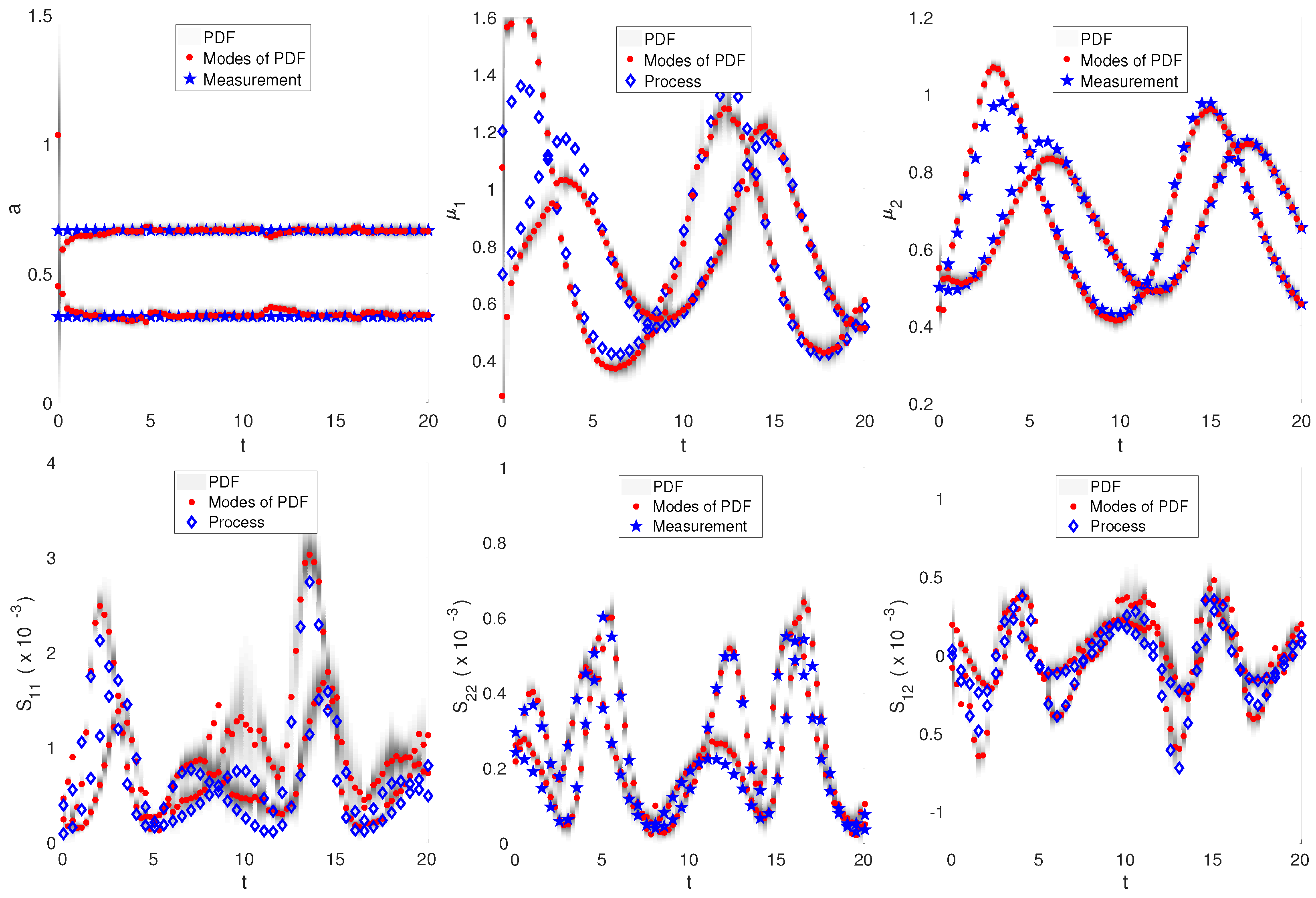
3.3. Nonlinear Dynamics: Intracellular Oscillator Modeled by Lotka–Volterra Dynamics

In the second benchmark, an intracellular oscillator was considered. Examples for such oscillatory behavior are found for example in the modeling of homeostasis and the cell cycle (see [31] and the references therein). It was assumed that the cell population exhibited variability with respect to two unspecified intracellular properties. Their coupled behavior was characterized by a Lotka–Volterra-type dynamics. As in the first benchmark, only the second cellular property was accessible. Thus, the following set of systems equations was obtained:

$$\begin{array}{cc}\hfill {\dot{z}}_1& =k_1{z}_1-k_2{z}_1{z}_2,\hfill \\ \hfill {\dot{z}}_2& =-k_3{z}_2+k_4{z}_1{z}_2,\hfill \\ \hfill y_z& =z_2.\hfill \end{array}$$

(39)

This also means that only projections to $z_2$ were measurable for the overall cell population number density function. Thus, after applying the proposed GMD approximation of the NDF, the following set of measurements was obtained:

$$\begin{array}{c}\hfill {\mathbf{y}}^{\left(i\right)}={\left(a^{\left(i\right)},{\mu }_2^{\left(i\right)},{\Sigma }_{2,2}^{\left(i\right)}\right)}^T,i=1,\dots ,N_{GMD}\end{array}$$

(40)

In contrast to the previous example, no closed set of equations was found to describe the evolution of Gaussians from one sample point to the next. Therefore, an approximate moment method based on the direct quadrature method of moments [20] was implemented: therein, each Gaussian was represented by a set of random sampling points. These were propagated by the nonlinear intracellular dynamics. The propagated samples themselves were approximated with a new Gaussian. The overall procedure was rather complex, and a direct function $\mathbf{f}\left(\mathbf{x}\right)$ was not determined easily. Hence, it was hardly possible to check for nonlinear observability of the cell population with the methods introduced previously. However, the nonlinear single cell dynamics were (weakly) observable, and the weak observability of individual Gaussians has been conjectured. In the implementation of the resampling step of the particle filter, a rather simple static normal distribution was implemented as the kernel function. All parameter values used in the numerical implementation are reported in Table 2.

Simulation results are depicted in Figure 3. The set of particles represents the PDF of the estimated state vector (depicted in grey scale, darker areas indicating regions of higher particle density). The measurements (and also the cell populations NDF) were approximated by two GMDs. Initially, the particles were evenly distributed (broad PDF), reflecting the uncertainty about the current state of the process. However, after a short period, a bimodal PDF was obtained indicating that the particles had focused within two regions. The PDF modes represent the particle filters’ estimates for the state vectors. It can be seen that most states were accurately estimated. In general, the estimates of mixture components and means seemed to be more reliable than the estimates of the covariance. Here, the estimate for $S_{1,1}$, i.e., the variance with respect to non-measurable component $z_1$, shows some significant deviations at some time points. The simulation showed that the estimates became worse for periods in which the two measurement GMDs overlapped, yielding a kind of practical non-observability. This was particularly obvious in the period $8<t<12$ where the uncertainty in the estimates increased (the PDF became broader), and the PDF modes did not represent good estimates for the measurements any longer. However, after a short time, the estimator was able to recover. It is also clear that the particle filter had to converge before a new critical practical non-observability situation arose. It has to be mentioned that the implemented particle filter algorithm was relatively simple and could be improved further by taking into account advanced techniques, e.g., different resampling strategies and improved particle prediction steps [13]. Another point for fine-tuning of the performance was found in the approximate moment method for the prediction of the state vectors: here, a more complex approximate moment closures could be considered.

4. Conclusions

This contribution proposed a novel approach to model-based online state estimation for multicellular systems from snapshot data. In classical approaches, state estimators are designed for grid-based discrete approximations of the involved PBEs. This approach is not favorable for multicellular systems: here, modeling is based on single cell kinetics commonly involving a high number of cellular states. As each of these states translates directly into one independent coordinate of the corresponding PBE, generally high-dimensional partial differential equations are obtained. Application of the grid-based discrete method would involve out-of-scale computational costs. In contrast, the proposed technique is based on an approximation of the cell number density distribution and snapshot measurements by Gaussian mixture densities. These are characterized by integral quantities, namely the mixture component (zeroth order moment), mean (first order moments) and covariance (centralized second order moments). In an online estimation, those are reconstructed instead of the full NDF. Thereby, the estimation is reduced from an infinite to a low dimensional problem, which enables the application of established estimator techniques, like Kalman and particle filtering. Dynamic equations for the integral quantities have to be derived from the PBE. Here, a closed set of equations is only found under special conditions, and approximate moment methods have to be implemented. The proposed framework also ensures a degree of flexibility with respect to the specific approximate moment method, as well as the specific estimator. Furthermore, well-known observability criteria from systems theory can be employed. Within two benchmark studies, the performance of Kalman and particle filters for the reconstruction of non-measurable properties of the cellular system was analyzed. In the first, a closed set of ODEs was used to compute means and covariances for linear cellular dynamics, while an approximate moment method was used in the second benchmark, which involved nonlinear cellular dynamics. The results indicate that the proposed approach represents a promising tool for online reconstruction of non-measurable cellular properties, which may also be extended to other multicellular processes with non-negligible cell death and cell division. Even though the proposed estimation technique is shown for the approximation of the full NDF with Gaussian mixture densities in this contribution, the general procedure could also be adopted for different mixture densities, e.g., Gamma distributions [32]. As for the second nonlinear benchmark, dynamics of the integral distribution quantities could be determined with an approximate moment method. Furthermore, it has to be mentioned that the introduced technique could also be applied to other particulate processes, e.g., particle formation or crystallization, which will be investigated in the future.

References

- Herberg, M.; Glauche, I.; Zerjatke, T.; Winzi, M.; Buchholz, F.; Roeder, I. Dissecting mechanisms of mouse embryonic stem cells heterogeneity through a model-based analysis of transcription factor dynamics. J. R. Soc. Interface 2016, 13, 201160167. [Google Scholar] [CrossRef] [PubMed]
- Müller, T.; Dürr, R.; Isken, B.; Schulze-Horsel, J.; Reichl, U.; Kienle, A. Distributed modeling of human influenza a virus-host cell interactions during vaccine production. Biotechnol. Bioeng. 2013, 110, 2252–2266. [Google Scholar] [CrossRef] [PubMed]
- Tapia, F.; Vázquez-Ramírez, D.; Genzel, Y.; Reichl, U. Bioreactors for high cell density and continuous multi-stage cultivations: Options for process intensification in cell culture-based viral vaccine production. Appl. Microbiol. Biotechnol. 2016, 100, 2121–2132. [Google Scholar] [CrossRef] [PubMed]
- Franz, A.; Dürr, R.; Kienle, A. Population Balance Modeling of Biopolymer Production in Cellular Systems. IFAC Proc. Vol. 2014, 47, 1705–1710. [Google Scholar] [CrossRef]
- Nopens, I.; Torfs, E.; Ducoste, J.; Vanrolleghem, P.; Gernaey, K. Population balance models: A useful complementary modelling framework for future WWTP modelling. Water Sci. Technol. 2015, 71, 159–167. [Google Scholar] [CrossRef]
- Pigou, M.; Morchain, J. Investigating the interactions between physical and biological heterogeneities in bioreactors using compartment, population balance and metabolic models. Chem. Eng. Sci. 2015, 126, 267–282. [Google Scholar] [CrossRef] [Green Version]
- Liou, J.; Fredrickson, A.G.; Srienc, F. Selective synchronization of Tetrahymena pyriformis cell populations and cell growth kinetics during the cell cycle. Biotechnol. Prog. 1998, 14, 450–456. [Google Scholar] [CrossRef] [PubMed]
- Müller, S.; Harms, H.; Bley, T. Origin and analysis of microbial population heterogeneity in bioprocesses. Curr. Opin. Biotechnol. 2010, 21, 100–113. [Google Scholar] [CrossRef] [PubMed]
- Binder, D.; Drepper, T.; Jaeger, K.E.; Delvigne, F.; Wiechert, W.; Kohlheyer, D.; Grünberger, A. Homogenizing bacterial cell factories: Analysis and engineering of phenotypic heterogeneity. Metab. Eng. 2017, 42, 145–156. [Google Scholar] [CrossRef] [PubMed]
- de Vargas Roditi, L.; Claassen, M. Computational and experimental single cell biology techniques for the definition of cell type heterogeneity, interplay and intracellular dynamics. Curr. Opin. Biotechnol. 2015, 34, 9–15. [Google Scholar] [CrossRef] [PubMed]
- Hasenauer, J.; Waldherr, S.; Doszczak, M.; Radde, N.; Scheurich, P.; Allgöwer, F. Identification of models of heterogeneous cell populations from population snapshot data. BMC Bioinform. 2011, 12, 125. [Google Scholar] [CrossRef] [PubMed]
- Natarajan, A.; Srienc, F. Glucose uptake rates of single E. coli cells grown in glucose-limited chemostat cultures. J. Microbiol. Methods 2000, 42, 87–96. [Google Scholar] [CrossRef]
- Simon, D. Optimal State Estimation: Kalman, H Infinity, and Nonlinear Approaches; John Wiley & Sons, Inc.: Hoboken, NJ, USA, 2006. [Google Scholar]
- Fredrickson, A.G.; Ramkrishna, D.; Tsuchiya, H.M. Statistics and dynamics of procaryotic cell populations. Math. Biosci. 1967, 1, 327–374. [Google Scholar] [CrossRef]
- Mangold, M. Use of a Kalman filter to reconstruct particle size distributions from FBRM measurements. Chem. Eng. Sci. 2012, 70, 99–108. [Google Scholar] [CrossRef]
- McLachlan, G.; Peel, D. Finite Mixture Models; Wiley Series in Probability And Statistics; John Wiley & Sons, Inc.: Hoboken, NJ, USA, 2000. [Google Scholar]
- Slack, M.D.; Martinez, E.D.; Wu, L.F.; Altschuler, S.J. Characterizing heterogeneous cellular responses to perturbations. Proc. Natl. Acad. Sci. USA 2008, 105, 19306–19311. [Google Scholar] [CrossRef] [PubMed] [Green Version]
- Altschuler, S.J.; Wu, L.F. Cellular Heterogeneity: Do Differences Make a Difference? Cell 2010, 141, 559–563. [Google Scholar] [CrossRef] [PubMed]
- Hasenauer, J.; Hasenauer, C.; Hucho, T.; Theis, F.J. ODE Constrained Mixture Modelling: A Method for Unraveling Subpopulation Structures and Dynamics. PLoS Comput. Biol. 2014, 10, e1003686. [Google Scholar] [CrossRef] [PubMed]
- Dürr, R.; Müller, T.; Duvigneau, S.; Kienle, A. An efficient approximate moment method for multi-dimensional population balance models—Application to virus replication in multi-cellular systems. Chem. Eng. Sci. 2017, 160, 321–334. [Google Scholar] [CrossRef]
- Ramkrishna, D. Population Balances: Theory and Applications to Particulate Systems in Engineering; Academic Press: San Diego, CA, USA, 2000. [Google Scholar]
- Luenberger, D. An introduction to observers. IEEE Trans. Autom. Control 1971, 16, 596–602. [Google Scholar] [CrossRef]
- Zeitz, M. Observability canonical (phase-variable) form for non-linear time-variable systems. Int. J. Syst. Sci. 1984, 15, 949–958. [Google Scholar] [CrossRef]
- Blanke, M.; Kinnaert, M.; Lunze, J.; Staroswiecki, M.; Schröder, J. Diagnosis and Fault-Tolerant Control, 3rd ed.; Springer-Verlag: Berlin/Heidelberg, Germany, 2016. [Google Scholar]
- Liu, Y.Y.; Slotine, J.J.; Barabási, A.L. Observability of complex systems. Proc. Natl. Acad. Sci. USA 2013, 110, 2460–2465. [Google Scholar] [CrossRef] [PubMed] [Green Version]
- Mangold, M.; Bück, A.; Schenkendorf, R.; Steyer, C.; Voigt, A.; Sundmacher, K. Two state estimators for the barium sulfate precipitation in a semi-batch reactor. Chem. Eng. Sci. 2009, 64, 646–660. [Google Scholar] [CrossRef]
- Zeng, S.; Waldherr, S.; Ebenbauer, C.; Allgöwer, F. Ensemble Observability of Linear Systems. IEEE Trans. Autom. Control 2016, 61, 1452–1465. [Google Scholar] [CrossRef]
- Wang, X.; Li, T.; Sun, S.; Corchado, J.M. A Survey of Recent Advances in Particle Filters and Remaining Challenges for Multitarget Tracking. Sensors 2017, 17, 2707. [Google Scholar] [CrossRef] [PubMed]
- Gerards, A. Chapter 3: Matching. In Network Models; Elsevier: Amsterdam, The Netherlands, 1995; Volume 7, pp. 135–224. [Google Scholar]
- Higham, D.J. An Algorithmic Introduction to Numerical Simulation of Stochastic Differential Equations. SIAM Rev. 2001, 43, 525–546. [Google Scholar] [CrossRef] [Green Version]
- Drengstig, T.; Ni, X.Y.; Thorsen, K.; Jolma, I.W.; Ruoff, P. Robust Adaptation and Homeostasis by Autocatalysis. J. Phys. Chem. B 2012, 116, 5355–5363. [Google Scholar] [CrossRef] [PubMed]
- Isensee, J.; Diskar, M.; Waldherr, S.; Buschow, R.; Hasenauer, J.; Prinz, A.; Allgöwer, F.; Herberg, F.W.; Hucho, T. Pain modulators regulate the dynamics of PKA-RII phosphorylation in subgroups of sensory neurons. J. Cell Sci. 2014, 127, 216–229. [Google Scholar] [CrossRef] [PubMed]
Figure 1.
(Left) Two-dimensional cell distribution; only individual size is measurable, but not growth rate; (right) model-based online estimation.
Figure 2.
Benchmark 1: protein expression, ; reconstruction of integral quantities of GMDs using Kalman filters and the Hungarian algorithm for data association.
Figure 3.
Benchmark 2: Lotka–Volterra dynamics, ; reconstruction of integral quantities of GMDs using particle filter: modes of the PDF (red) represent estimates of the GMDs (only each second measurement (blue) is depicted to improve visibility).