Nutrient Diagnosis of Eucalyptus at the Factor-Specific Level Using Machine Learning and Compositional Methods

 ,
,  ,
,
Abstract
:
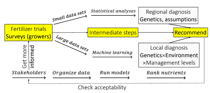
1. Introduction
2. Materials and Methods
2.1. Data Set
2.2. Fertilization
2.3. Plant Measurements and Analysis
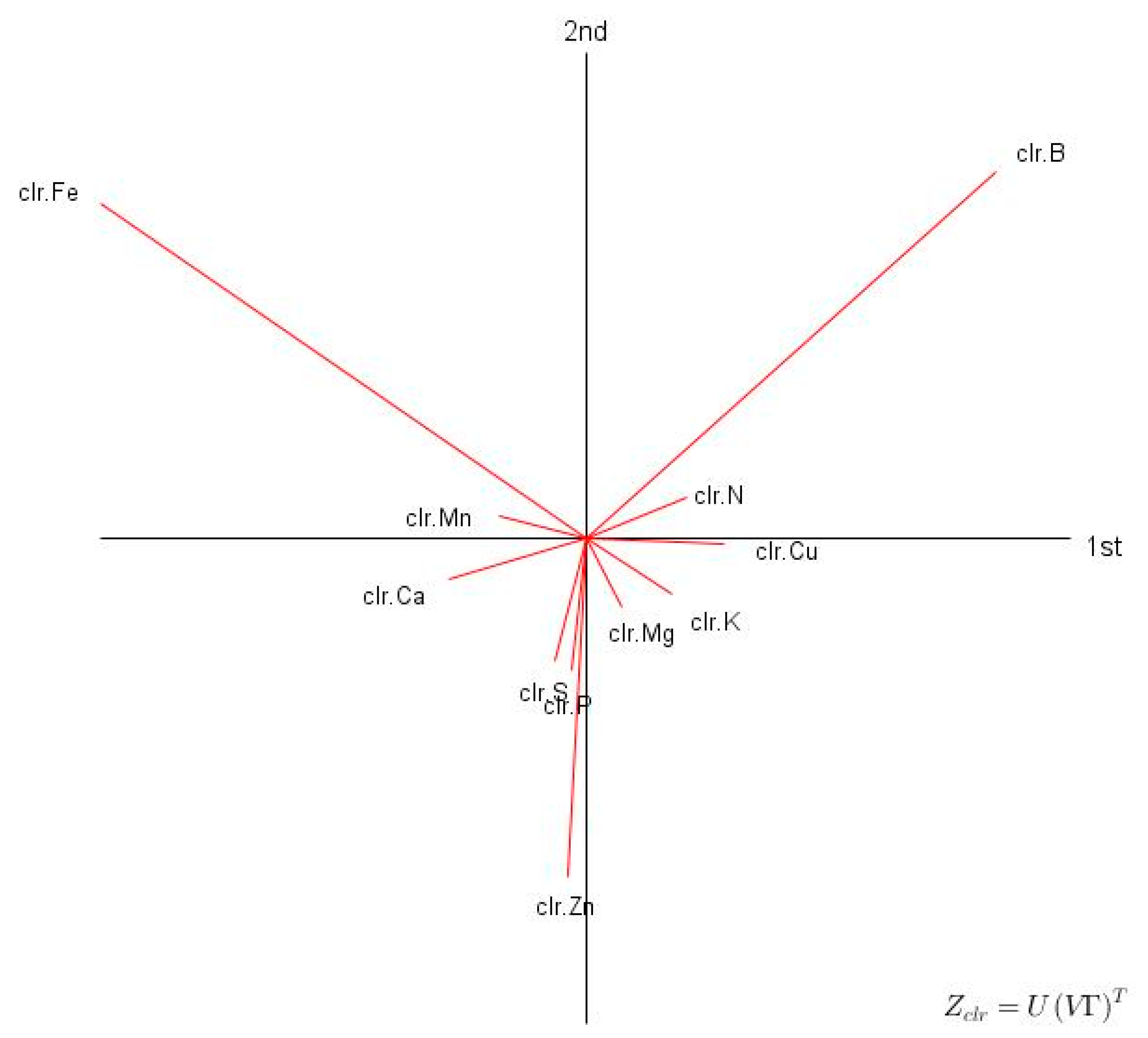
2.4. Log-Ratio Transformation Techniques
2.5. Regional Diagnosis
2.6. Local Diagnosis
2.7. Statistical Analysis
3. Results
3.1. Descriptive Statistics and Exploratory Analyses
3.2. Machine Learning Models
3.3. Nutrient Intervals at a Regional Scale
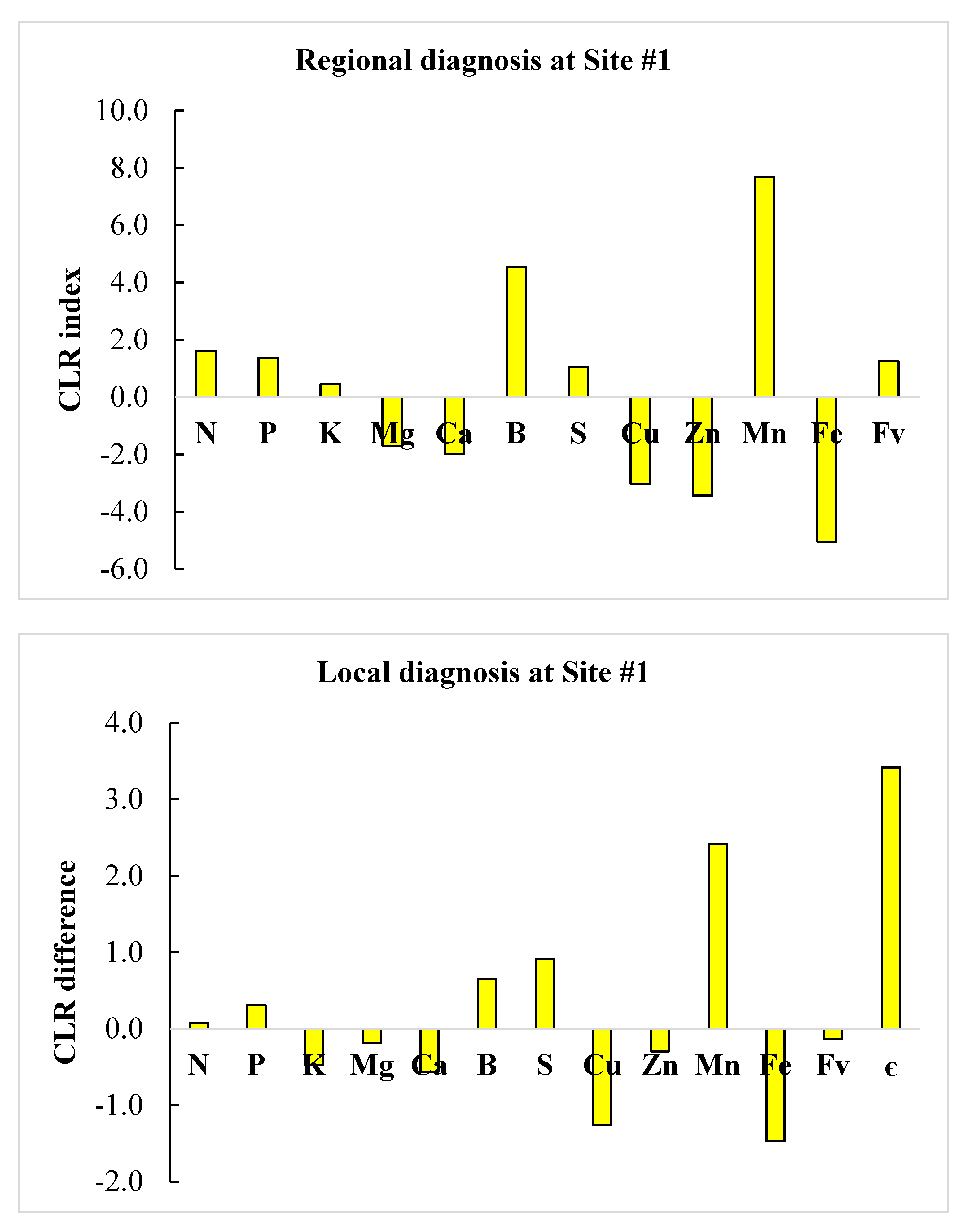
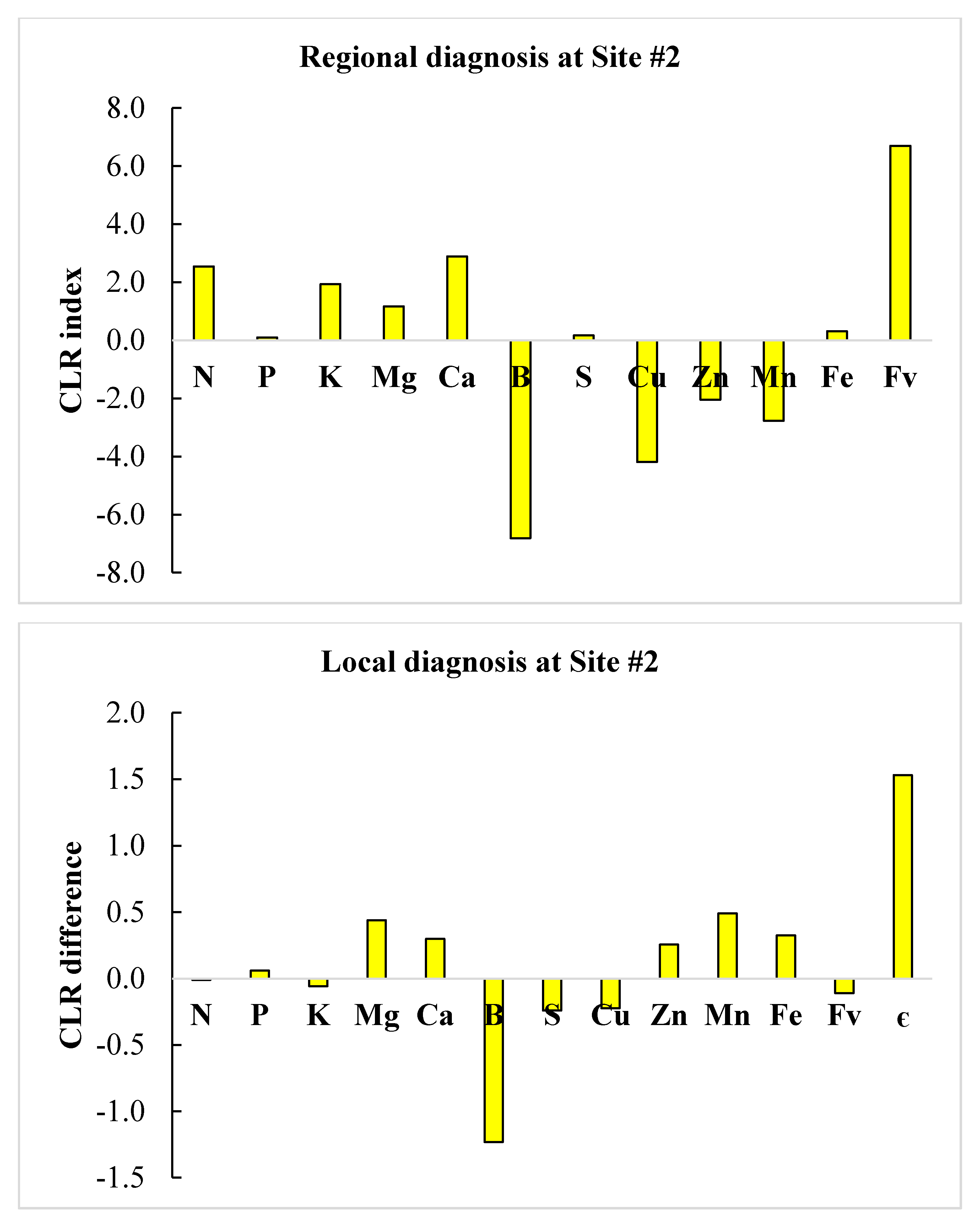
3.4. Regional vs. Local Diagnosis
4. Discussion
4.1. ML Model
4.2. Compositions as Unique Combinations of Nutrients
5. Conclusions
Author Contributions
Funding
Conflicts of Interest
References
- Laclau, J.P. Eucalyptus 2018: Managing Eucalyptus Plantations under Global Changes, 1st ed.; IUFRO, Ed.; Montpellier: Le Corum, France, 2018; ISBN 978-2-87614-743-0. [Google Scholar]
- IBÁ Relatório Anual 2017. Available online: https://iba.org/images/shared/Biblioteca/IBA_RelatorioAnual2017.pdf (accessed on 10 July 2019).
- Clearwater, M.J.; Meinzer, F.C. Relationships between hydraulic architecture and leaf photosynthetic capacity in nitrogen-fertilized Eucalyptus grandis trees. Tree Physiol. 2001, 21, 683–690. [Google Scholar] [CrossRef]
- Graciano, C.; Goya, J.F.; Frangi, J.L.; Guiamet, J.J. Fertilization with phosphorus increases soil nitrogen absorption in young plants of Eucalyptus grandis. For. Ecol. Manag. 2006, 236, 202–210. [Google Scholar] [CrossRef]
- Laclau, J.-P.; Almeida, J.C.R.; Goncalves, J.L.M.; Saint-Andre, L.; Ventura, M.; Ranger, J.; Moreira, R.M.; Nouvellon, Y. Influence of nitrogen and potassium fertilization on leaf lifespan and allocation of above-ground growth in Eucalyptus plantations. Tree Physiol. 2008, 29, 111–124. [Google Scholar] [CrossRef]
- Gazola, R.d.N.; Buzetti, S.; Teixeira Filho, M.C.M.; Gazola, R.P.D.; Celestrino, T.D.S.; Silva, A.C.D.; Silva, P.H.M.D. Potassium fertilization of eucalyptus in an entisol in low-elevation cerrado. Rev. Bras. Ciência do Solo 2019, 43. [Google Scholar] [CrossRef] [Green Version]
- Hubbard, R.M.; Ryan, M.G.; Giardina, C.P.; Barnard, H. The effect of fertilization on sap flux and canopy conductance in a Eucalyptus saligna experimental forest. Glob. Chang. Biol. 2004, 10, 427–436. [Google Scholar] [CrossRef]
- Viera, M.; Ruíz Fernández, F.; Rodríguez-Soalleiro, R. Nutritional prescriptions for eucalyptus plantations: Lessons learned from spain. Forests 2016, 7, 84. [Google Scholar] [CrossRef] [Green Version]
- Stape, J.L.; Binkley, D.; Ryan, M.G.; Fonseca, S.; Loos, R.A.; Takahashi, E.N.; Silva, C.R.; Silva, S.R.; Hakamada, R.E.; Ferreira, J.M.d.A.; et al. The Brazil eucalyptus potential productivity project: Influence of water, nutrients and stand uniformity on wood production. For. Ecol. Manag. 2010, 259, 1684–1694. [Google Scholar] [CrossRef]
- Munson, R.D.; Nelson, W.L. Principles and Practices in Plant Analysis. In Soil Testing and Plant Analysis; Westerman, R.L., Ed.; Soil Science Society of America, Inc.: Madison, WI, USA, 1990; pp. 359–387. [Google Scholar]
- Gatiboni, L.C.; Da Ros, C.O.; Stahl, S.; Araújo, E.F. Adubação de Eucalipto. In Manual de Calagem e Adubação do RS/SC; Silva, L.S., Ed.; Comissão de Química e Fertilidade: Alegre, Brazil, 2016; pp. 245–247. [Google Scholar]
- Ferreira, E.V.d.O.; Novais, R.F.; Médice, B.M.; de Barros, N.F.; Silva, I.R. Leaf total nitrogen concentration as an indicator of nitrogen status for plantlets and young plants of Eucalyptus clones. Rev. Bras. Ciência do Solo 2015, 39, 1127–1140. [Google Scholar] [CrossRef] [Green Version]
- de Morais, T.C.B.; Prado, R.D.M.; Traspadini, E.I.F.; Wadt, P.G.S.; de Paula, R.C.; Rocha, A.M.S. Efficiency of the CL, DRIS and CND Methods in assessing the nutritional status of eucalyptus spp. rooted cuttings. Forests 2019, 10, 786. [Google Scholar] [CrossRef] [Green Version]
- da Silva, G.G.C.; Neves, J.C.L.; Alvarez, V.V.H.; Leite, F.P. Nutritional diagnosis for eucalypt by DRIS, M-DRIS, and CND. Sci. Agric. 2004, 61, 507–515. [Google Scholar] [CrossRef] [Green Version]
- Aitchison, J. The statistical analysis of compositional data. J. R. Stat. Soc. Ser. B 1982, 44, 139–160. [Google Scholar] [CrossRef]
- Amrhein, V.; Greenland, S.; McShane, B. Retire statistical significance. Nature 2019, 567, 305–307. [Google Scholar] [CrossRef] [PubMed] [Green Version]
- Walworth, J.L.; Sumner, M.E. The diagnosis and recommendation integrated system (DRIS). Adv. Soil Sci. 1987, 6, 149–188. [Google Scholar] [CrossRef]
- Betemps, D.L.; de Paula, B.V.; Parent, S.-É.; Galarça, S.P.; Mayer, N.A.; Marodin, G.A.B.; Rozane, D.E.; Natale, W.; Melo, G.W.B.; Parent, L.E.; et al. Humboldtian diagnosis of peach tree (prunus persica) nutrition using machine-learning and compositional methods. Agronomy 2020, 10, 900. [Google Scholar] [CrossRef]
- Umesh, U.N.; Peterson, R.A.; McCann-Nelson, M.; Vaidyanathan, R. Type IV error in marketing research: The investigation of ANOVA interactions. J. Acad. Mark. Sci. 1996, 24, 17–26. [Google Scholar] [CrossRef]
- Wallace, A.; Wallace, G.A. Horticultural Review; Janick, J., Ed.; John Wiley & Sons, Inc.: Oxford, UK, 1993; ISBN 9780470650547. [Google Scholar]
- Adams, M.; Rennenberg, H.; Kruse, J. Resilience of primary metabolism of eucalypts to variable water and nutrients. In Eucalyptus 2018: Managing Eucalyptus Plantations under Global Changes; Montpellier: Le Corum, France, 2018; pp. 100–104. ISBN 978-2-87614-743-0. [Google Scholar]
- Aspinwall, M.; Blackman, C.; Resco De Dios, V.; Tjoelker, M.; Tissue, D. Photosynthesis and carbon allocation are both important predictors of genotype productivity responses to elevated CO2 in Eucalyptus camaldulensis. In Eucalyptus 2018: Managing Eucalyptus Plantations under Global Changes; Montpellier: Le Corum, France, 2018; pp. 106–110. ISBN 978-2-87614-743-0. [Google Scholar]
- Keppel, G.; Kreft, H. Integration and synthesis of quantitative data: Alexander von Humboldt’s renewed relevance in modern biogeography and ecology. Front. Biogeogr. 2019, 11. [Google Scholar] [CrossRef] [Green Version]
- Olden, J.D.; Lawler, J.J.; Poff, N.L. Machine learning methods without tears: A Primer for ecologists. Q. Rev. Biol. 2008, 83, 171–193. [Google Scholar] [CrossRef] [Green Version]
- Shalev-Shwartz, S.; Ben-David, S. Understanding Machine Learning: From Theory to Algorithms, 1st ed.; Cambridge University Press: New York, NY, USA, 2014; ISBN 978-1-107-05713-5. [Google Scholar]
- Parent, S.-É. Why we should use balances and machine learning to diagnose ionomes. Authorea 2020, 1. [Google Scholar] [CrossRef]
- Coulibali, Z.; Cambouris, A.N.; Parent, S.-É. Cultivar-specific nutritional status of potato (Solanum tuberosum L.) crops. PLoS ONE 2020, 15, e0230458. [Google Scholar] [CrossRef] [Green Version]
- de Wit, C.T. Resource use efficiency in agriculture. Agric. Syst. 1992, 40, 125–151. [Google Scholar] [CrossRef]
- Grunsky, E.C.; de Caritat, P. State-of-the-art analysis of geochemical data for mineral exploration. Geochem. Explor. Environ. Anal. 2020, 20, 217–232. [Google Scholar] [CrossRef]
- Martín-Fernández, J.A.; Barceló-Vidal, C.; Pawlowsky-Glahn, V. Dealing with zeros and missing values in compositional data sets using nonparametric imputation. Math. Geol. 2003, 35, 253–278. [Google Scholar] [CrossRef]
- Egozcue, J.J.; Pawlowsky-Glahn, V.; Mateu-Figueras, G.; Barceló-Vidal, C. Isometric logratio transformations for compositional data analysis. Math. Geol. 2003, 35, 279–300. [Google Scholar] [CrossRef]
- Köppen, W.; Geiger, G. Klima Der Erde (Map) 1954. Available online: http://koeppen-geiger.vu-wien.ac.at (accessed on 3 March 2020).
- Santos, H.G. Sistema Brasileiro de Classificação de Solos, 5th ed.; Embrapa: Brasilia, Brazil, 2018; ISBN 978-85-7035-800-4. [Google Scholar]
- Tedesco, M.J.; Gianello, C.; Bissani, C.A.; Bohnen, H. Análises de Solo, Plantas e Outros Materiais; UFRGS: Porto Alegre, Brazil, 1995. [Google Scholar]
- Tolosana-Delgado, R.; Talebi, H.; Khodadadzadeh, M.; Van den Boogaart, K.G. On machine learning algorithms and compositional data. In Proceedings of the 8th International Workshop on Compositional Data Analysis, Terrassa, Spain, 3–8 June 2019; Egozcue, J.J., Graffelman, J., Ortego, M.I., Eds.; pp. 172–175. [Google Scholar]
- Budhu, M. Soil Mechanics and Foundations, 3rd ed.; Wiley: New York, NY, USA, 2010; Volume 1, ISBN 9788578110796. [Google Scholar]
- Parent, L.E.; Dafir, M. A theoretical concept of compositional nutrient diagnosis. J. Am. Soc. Hortic. Sci. 1992, 117, 239–242. [Google Scholar] [CrossRef] [Green Version]
- Beaufils, E. Diagnosis and Recommendation Integrated System (DRIS), 1st ed.; University of Natal: Pietermaritzburg, South Africa, 1973. [Google Scholar]
- Badra, A.; Parent, L.-É.; Allard, G.; Tremblay, N.; Desjardins, Y.; Morin, N. Effect of leaf nitrogen concentration versus CND nutritional balance on shoot density and foliage colour of an established Kentucky bluegrass (Poa pratensis L.) turf. Can. J. Plant Sci. 2006, 86, 1107–1118. [Google Scholar] [CrossRef]
- Aitchison, J. Principles of compositional data analysis. Multivar. Anal. Its Appl. IMS Lect. Notes Monogr. Ser. 1994, 24, 73–81. [Google Scholar]
- Rodgers, J.L.; Nicewander, W.A.; Toothaker, L. Linearly independent, orthogonal, and uncorrelated variables. Am. Stat. 1984, 38, 133. [Google Scholar] [CrossRef]
- Filzmoser, P.; Hron, K.; Reimann, C. Univariate statistical analysis of environmental (compositional) data: Problems and possibilities. Sci. Total Environ. 2009, 407, 6100–6108. [Google Scholar] [CrossRef]
- Egozcue, J.J.; Pawlowsky-Glahn, V. Groups of parts and their balances in compositional data analysis. Math. Geol. 2005, 37, 795–828. [Google Scholar] [CrossRef] [Green Version]
- de Oliveira, C.T.; Rozane, D.E.; de Amorim, D.A.; de Souza, H.A.; Fernandes, B.S.; Natale, W. Diagnosis of the nutritional status of ‘Paluma’ guava trees using leaf and flower analysis. Rev. Bras. Frutic. 2020, 42, 1–9. [Google Scholar] [CrossRef]
- Breiman, L. Random forests. Mach. Learn. 2001, 45, 5–32. [Google Scholar]
- Delacour, H.; Servonnet, A.; Perrot, A.; Vigezzi, J.F.; Ramirez, J.M. La courbe ROC (receiver operating characteristic): Principes et principales applications en biologie clinique. Ann. Biol. Clin. (Paris) 2005, 63, 145–154. [Google Scholar]
- Parent, S.-É.; Parent, L.E.; Rozane, D.-E.; Natale, W. Plant ionome diagnosis using sound balances: Case study with mango (Mangifera Indica). Front. Plant Sci. 2013, 4, 449. [Google Scholar] [CrossRef] [PubMed] [Green Version]
- Parent, L.E.; Rozane, D.E.; Deus, J.A.L.; Natale, W. Diagnosis of nutrient composition in Fruit crops: Latest developments. In Fruit Crops. Diagnosis and Management of Nutrient Constraints; Srivastava, A.K., Hu, C., Eds.; Elsevier: New York, NY, USA, 2019; p. 400. [Google Scholar]
- Ryo, M.; Rillig, M.C. Statistically reinforced machine learning for nonlinear patterns and variable interactions. Ecosphere 2017, 8, e01976. [Google Scholar] [CrossRef]
- Nowaki, R.H.D.; Parent, S.-É.; Cecílio Filho, A.B.; Rozane, D.E.; Meneses, N.B.; Silva, J.A.; Natale, W.; Parent, L.E. Phosphorus over-fertilization and nutrient misbalance of irrigated tomato crops in Brazil. Front. Plant Sci. 2017, 8, 825. [Google Scholar] [CrossRef] [PubMed]
- Wilkinson, S.R.; Grunes, D.L.; Sumner, M.E. Nutrient interactions in soil and plant nutrition. In Handbook of Soil Fertility and Plant Nutrition; Sumner, M.E., Ed.; CRC Press: London, UK, 2000; p. 91. [Google Scholar]
- Marschner, P. Marschner ’ s Mineral Nutrition of Higher Plants, 3rd ed.; Academic Press: London, UK, 2012; ISBN 9780123849052. [Google Scholar]
- Barber, S.A. Soil Nutrient Bioavailability: A Mechanistic Approach, 2nd ed.; Wiley: New York, NY, USA, 1995. [Google Scholar]
- Gibson, K.J.; Streich, M.K.; Topping, T.S.; Stunz, G.W. Utility of citizen science data: A case study in land-based shark fishing. PLoS ONE 2019, 14, e0226782. [Google Scholar] [CrossRef]


| Component | Minimum | Median | Maximum |
|---|---|---|---|
| g kg−1 | |||
| N | 9.1 | 21.9 | 38.8 |
| P | 0.5 | 1.3 | 3.3 |
| K | 1.2 | 9.4 | 19.6 |
| Mg | 1.0 | 2.6 | 7.5 |
| Ca | 2.7 | 8.6 | 34.9 |
| S | 0.4 | 1.5 | 5.1 |
| B | 0.011 | 0.038 | 0.105 |
| Cu | 0.001 | 0.008 | 0.036 |
| Zn | 0.006 | 0.018 | 0.129 |
| Mn | 0.066 | 0.964 | 4.954 |
| Fe | 0.002 | 0.076 | 0.594 |
| Filling value | 925.6 | 952.1 | 973.3 |
| Expression | AUC | CA | TN | FN | FP | TP |
|---|---|---|---|---|---|---|
| Random Forests | 0.787 | 0.718 | 521 | 219 | 315 | 816 |
| Neural Networks | 0.778 | 0.705 | 548 | 271 | 278 | 764 |
| Naïve Bayes | 0.793 | 0.715 | 614 | 318 | 212 | 717 |
| Support Vector Machine | 0.544 | 0.529 | - | - | - | - |
| KNN | 0.589 | 0.570 | - | - | - | - |
| Adaboost | 0.636 | 0.641 | - | - | - | - |
| Stochastic Gradient Decent | 0.674 | 0.679 | - | - | - | - |
| Nutrient Expression | Area Under Curve | Classification Accuracy |
|---|---|---|
| Raw concentration data | 0.787 | 0.718 |
| Pairwise log ratios | 0.721 | 0.664 |
| Centered log ratios | 0.785 | 0.706 |
| Isometric log ratios | 0.776 | 0.701 |
| Nutrient | State (Gatiboni et al. [11]) | True Negative Quartiles (25, 75) | ||
|---|---|---|---|---|
| Lower bound | Upper bound | Lower bound | Upper bound | |
| g kg−1 | ||||
| N | 15.0 | 20.0 | 17.0 | 25.3 |
| P | 1.0 | 1.3 | 1.0 | 1.4 |
| K | 9.0 | 13.0 | 7.2 | 11.5 |
| Mg | 6.0 | 10.0 | 2.3 | 3.2 |
| Ca | 5.0 | 8.0 | 7.0 | 10.2 |
| S | 1.5 | 2.0 | 1.2 | 1.8 |
| mg kg−1 | ||||
| B | 30 | 50 | 6 | 12 |
| Cu | 7 | 10 | 14 | 21 |
| Zn | 35 | 50 | 60 | 96 |
| Mn | 400 | 600 | 34 | 54 |
| Fe | 150 | 200 | 679 | 1281 |
| Nutrient | Site #1 | Site #2 | Site #1 | Site #2 | ||
|---|---|---|---|---|---|---|
| g kg−1 | State Standards | TN Quartiles | State Standards | TN Quartiles | ||
| N | 27.1 | 15.0 | High | High | Normal | Low |
| P | 1.4 | 1.3 | High | Normal | Normal | Normal |
| K | 8.8 | 8.2 | Low | Normal | Low | Normal |
| Mg | 1.5 | 3.8 | Low | Low | Low | High |
| Ca | 3.9 | 21.2 | Low | Low | High | High |
| S | 1.7 | 1.4 | Normal | Normal | Low | Normal |
| mg kg−1 | Diagnosis | |||||
| B | 48.0 | 1.3 | Normal | High | Low | Low |
| Cu | 4.7 | 17.9 | Low | Low | High | Normal |
| Zn | 14.7 | 151.8 | Low | Low | High | High |
| Mn | 452.3 | 73.8 | Normal | High | Low | High |
| Fe | 66.9 | 1614.4 | Low | Low | High | High |
| Nutrient | 489 TN Specimens | |
|---|---|---|
| Mean | Standard Deviation | |
| N | 2.9050 | 0.3048 |
| P | 0.0726 | 0.2618 |
| K | 2.1387 | 0.2878 |
| Mg | 0.8880 | 0.2270 |
| Ca | 2.0454 | 0.2962 |
| B | −4.8438 | 0.4189 |
| S | 0.3053 | 0.3024 |
| Cu | −4.0882 | 0.3872 |
| Zn | −2.7212 | 0.4089 |
| Mn | −3.2629 | 0.3338 |
| Fe | −0.2132 | 0.4754 |
| Fv | 6.7743 | 0.1453 |
© 2020 by the authors. Licensee MDPI, Basel, Switzerland. This article is an open access article distributed under the terms and conditions of the Creative Commons Attribution (CC BY) license (http://creativecommons.org/licenses/by/4.0/).
Share and Cite
Vahl de Paula, B.; Squizani Arruda, W.; Etienne Parent, L.; Frank de Araujo, E.; Brunetto, G. Nutrient Diagnosis of Eucalyptus at the Factor-Specific Level Using Machine Learning and Compositional Methods. Plants 2020, 9, 1049. https://doi.org/10.3390/plants9081049
Vahl de Paula B, Squizani Arruda W, Etienne Parent L, Frank de Araujo E, Brunetto G. Nutrient Diagnosis of Eucalyptus at the Factor-Specific Level Using Machine Learning and Compositional Methods. Plants. 2020; 9(8):1049. https://doi.org/10.3390/plants9081049
Chicago/Turabian StyleVahl de Paula, Betania, Wagner Squizani Arruda, Léon Etienne Parent, Elias Frank de Araujo, and Gustavo Brunetto. 2020. "Nutrient Diagnosis of Eucalyptus at the Factor-Specific Level Using Machine Learning and Compositional Methods" Plants 9, no. 8: 1049. https://doi.org/10.3390/plants9081049