Probability Distribution Functions of Solar and Stellar Flares


National Astronomical Observatory of Japan, 2-21-1 Osawa, Mitaka, Tokyo 181-8588, Japan
Physics 2023, 5(1), 11-23; https://doi.org/10.3390/physics5010002
Submission received: 28 September 2022
/
Revised: 2 December 2022
/
Accepted: 14 December 2022
/
Published: 28 December 2022
(This article belongs to the Special Issue A Themed Issue in Honor of Professor Marcel Goossens on the Occasion of His 75th Birthday)
Abstract
:The paper studies the soft X-ray data of solar flares and found that the distribution functions of flare fluence are successfully modeled by tapered power law or gamma function distributions whose power exponent is slightly smaller than 2, indicating that the total energy of the flare populations is mostly due to a small number of large flares. The largest possible solar flares in 1000 years are predicted to be around X70 (a peak flux of 70 × 10−4 W m−2) in terms of the GOES (Geostationary Operational Environmental Satellites) flare class. The paper also studies superflares (more energetic than solar flares) from solar-type stars and found that their power exponent in the fitting of the gamma function distribution is around 1.05, which is much flatter than solar flares. The distribution function of stellar flare energy extrapolated downward does not connect to the distribution function of solar flare energy.
1. Introduction
Solar flares are the most energetic phenomena among a wide variety of magnetic activities taking place on the Sun [1,2]. The first flare observation was made by Carrington in 1859 in white light [3], and the earlier observations were restricted to Hα emission. Later radio and X-ray observations revealed that flares heat the corona from its normal 1–2 MK state to 10 MK or beyond. Then, it was found in 1980s that the largest fraction of energy in flares goes to the kinetic energy of coronal mass ejections (CMEs). The most energetic flares liberate energies up to 1033 erg [4]. Now it seems established that the energy release in solar flares is due to magnetic reconnection [5].
The number of flares, f(E)dE, with energies between E and E + dE is distributed roughly in power law [6,7] with a negative exponent, f(E)~E−α; i.e., smaller flares are more numerous. This property led Parker [8] to propose that the solar corona might be heated [9] by energies supplied from numerous small flares, later called nanoflares (in contrast to another class of theory based on waves [10,11]). Here, the important criterion is whether the power law index α is larger or smaller than 2 [12]. The total energy brought by all the flares with energies between E1 and E2 is
If α > 2, then contributions from smaller events (E1→0) determine the total energy involved in the flare phenomenon. However, for the observed flares of moderate or large sizes it is generally believed that α < 2 (1.8 or about). Therefore, more contributions to W come from larger flares. On the large energy end, in terms of space weather it has been discussed how frequent very large (extreme) events would happen [4]. Recent discovery of energetic flares (superflares) from solar-type (old and slowly rotating) stars [13,14] has stimulated interest in solar extreme events.
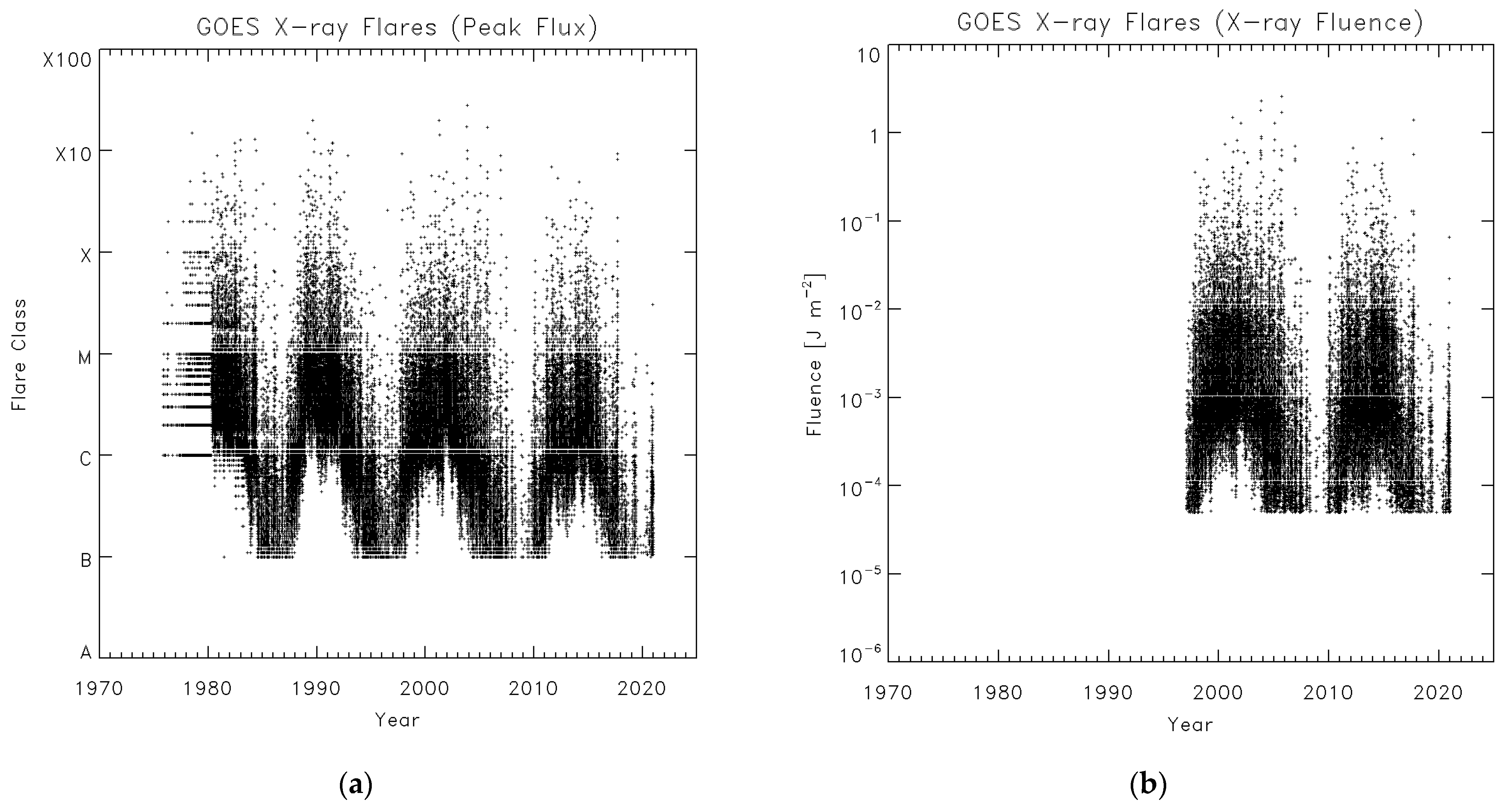
This study looks into the probability distribution functions of solar X-ray flares. As numerical measures both X-ray peak flux and X-ray fluence, which is the time integration of X-ray flux, are used. The peak X-ray flux may be subject to detector saturation for very large flares (X17 or larger [15]), but we expect that X-ray fluence data would suffer less influences because of time integration. The data used here are the soft X-ray observation by the Geostationary Operational Environmental Satellites (GOES) [16] (Figure 1). In Figure 1, 7.9 × 10⁴ flare events of peak flux above 10−7 W m−2 (1975–2020) and 3.4 × 10⁴ events of fluence above 5 × 10⁻⁵ J m−2 (1997–2020) are plotted.
In a foregoing study [17], the power law indices of α = 2.11 for X-ray peak flux and α = 2.03 for X-ray fluence were derived. Additionally, it was pointed out that α would be 1.88 if the background intensity is subtracted from the flare data.
The conclusions here are that although the distributions are roughly of a power law, at the high energy end they are tapered off exponentially. The power law is a scale-free distribution and could be a viable model for phenomena taking place in scales sufficiently smaller than the entire system (the Sun in the present case). Solar flares are powered by magnetic energy stored in sunspot regions, and since sunspot sizes cannot exceed the Sun (or more effectively limited by the depth of the convection zone), a limit is expected on the amount of energy released in flares. Therefore, a power-law extension of the distribution overestimates the frequency of extremely large solar flares. In Section 4, the energy distribution function of stellar flares is briefly discussed and compared with the solar flare case
2. Data and Methods
In this study, X-ray flux observed in the 0.1–0.8 nm band of the GOES X-ray sensors (1980–2020) is used. The peak flux values are traditionally expressed [18] in terms of A (10−8 W m−2), B (10−7 W m−2), C (10−6 W m−2), M (10−5 W m−2), and X (10−4 W m−2) classes. Namely, an M5.5 flare means a flare of peak flux 5.5 × 10⁻⁵ W m−2 and an X12 flare has a peak flux of 12 × 10−4 W m−2. The data are available from 1975, but the data before 1980 had one-digit accuracy (C2, M4, etc.); therefore, the data after 1980 which have two-digit accuracy (C2.1, M3.9, etc.) are used. The data after 1997 also include the fluence values (time integration of X-ray flux). In the following analysis flares with peak flux above M3 or 3 × 10⁻⁵ W m−2 (1980–2020, 1720 events) and also flares with fluence above 1 × 10⁻² J m−2 (1997–2020, 1945 events) are picked up (the data are available as described in the Supplementary Materials). The analysis uses the old operational scale instead of the new science scale adopted by the National Oceanic and Atmospheric Administration (NOAA) [15] (operational values = 0.7 × science values). The peak flux data of 2020 and the background data of 2011–2020 which were in the science database had been converted to the operational scale.
As previously suggested [17], background subtraction may significantly affect the data from small events particularly. Here, a simplified approach is adopted by subtracting the daily background value from the flare peak flux, and the value of the background times the duration from the fluence data (the duration of a flare can be computed from the flare start and end times given in the database). The background subtraction was not applied for 1980–1983 April (data not available) and on other days with no background data available, and when the background exceeds the flare intensity (e.g., when the background was too high because of a preceding flare).
The complementary cumulative distribution function, CCDF(F), of fluence F defined as [19]
is studied, where N = 1945 is the total number of events under study. The probability distribution function (PDF) is defined by
but here the flare occurrence rate is used defined by
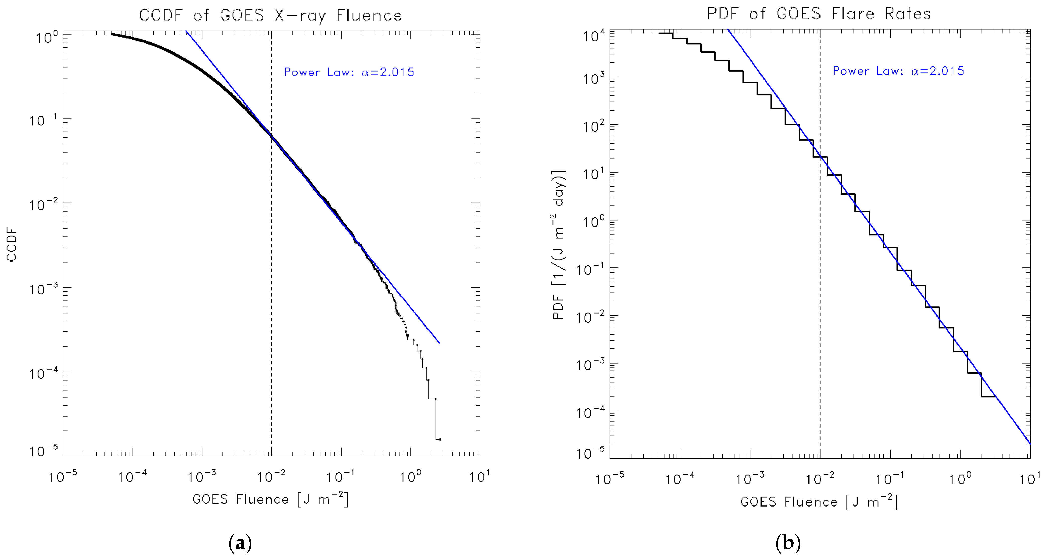
where τobs is the total duration of data (24 years). The dimension of f(F) is 1/(J m−2 day). Figure 2 shows CCDF(F) (Figure 2a) and f(F) (Figure 2b).
CCDF(F) = n(fluence ≥ F)/N,
One can likewise define the quantities for X-ray peak flux Fp, with Np = 1720 and τobs,p = 41 years. The dimension of f(Fp) is 1/(W m−2 day).
Let us fit the observed CCDF by four kinds of models: power law, tapered power law, gamma function, and Weibull distributions. The power law distribution is defined by [19]
where α > 1 and F0 (=1 × 10⁻² J m−2; F0p = 3 × 10⁻⁵ W m−2 for the peak flux data) is the lower boundary of the fitting. The other three are two-parameter models. The tapered power law distribution is defined by [20]
where α > 1, β > 0. The gamma function distribution is defined by [20]
where α > 1, β > 0, and Γ is the incomplete gamma function. The CCDF of the gamma function distribution is given as
The tapered power law and gamma function distributions have been used in geophysics in representing the distributions of earthquake magnitudes [21], in contrast to the power law distribution which is called the Gutenberg–Richter relation in seismology [22,23].
The Weibull distribution is defined by
where k > 0, β > 0. The Weibull distribution was first introduced to evaluate the failure rates of industrial products [24].
The parameters can be determined by using the maximum likelihood method, namely by maximizing the log-likelihood (LLH) defined by
Specific forms of the maximum-likelihood solutions can be found in the literature for power law [19], tapered power law [25], gamma function [20], and Weibull [26] distributions. The goodness of fit can be evaluated by the Kolmogorov–Smirnov (K-S) test [27], which uses the maximum difference between the observed and theoretical CCDFs. Whether one model is superior to the others can be estimated by Akaike’s Information Criterion (AIC) [28] given by
where K is the number of parameters used for fitting (K = 1 for power law; K = 2 for the other three models). By introducing more parameters, the fitting will improve, and one may obtain a larger LLH, but meaningful improvement requires that AIC decreases sufficiently (reduction in AIC of about 9–11 [29]). A similar analysis was conducted by the author on the area distribution of sunspots [30].
AIC = −2∙LLH + 2K,
Statistical errors in the determined parameter values can be estimated by generating many statistical distributions from the same parameter values and by seeing the distributions of the fitted parameter values (parametric bootstrap method [31]).
3. Results
Table 1 and Table 2 summarize the fitting results for X-ray fluence and peak flux, respectively. The errors given in Table 1 and Table 2 are the one-sigma (one-standard-deviation) errors thus derived.
ΔAIC is the difference in AIC from the smallest AIC value (indicating the most likely model) among all the models, and models with ΔAIC 9–11 are poorly supported compared to the ΔAIC = 0 model. Therefore, we can conclude that the power law model, shown in Figure 3, is not favorable compared to the other two-parameter models.
A model can be rejected by the K-S test by examining its measure, √N × KS, where KS is the maximum difference between the observed and model CCDFs. The probability that the observed √N ×KS value or larger is obtained (the “KS p-value” in Table 1 and Table 2) is given analytically as the Kolmogorov–Smirnov function which has only a weak dependence on √N regardless of the models assumed [32]. If the value of √N F0× KS is large and the corresponding KS p-value is small, one can conclude that the model is rejected. However, it is found here that the KS measures are generally small, and the p-values are not so small even for the power-law models. This happens because the K-S test is not sensitive to misfitting at the tail of the distributions. If F0 value is reduced, the fitting degrades and eventually all the models tend to be rejected by the K-S test. The ambiguities in setting the lower bound F0 of the probability distribution function are discussed in Section 4.
3.1. Tapered Power Law and Gamma Function Distributions
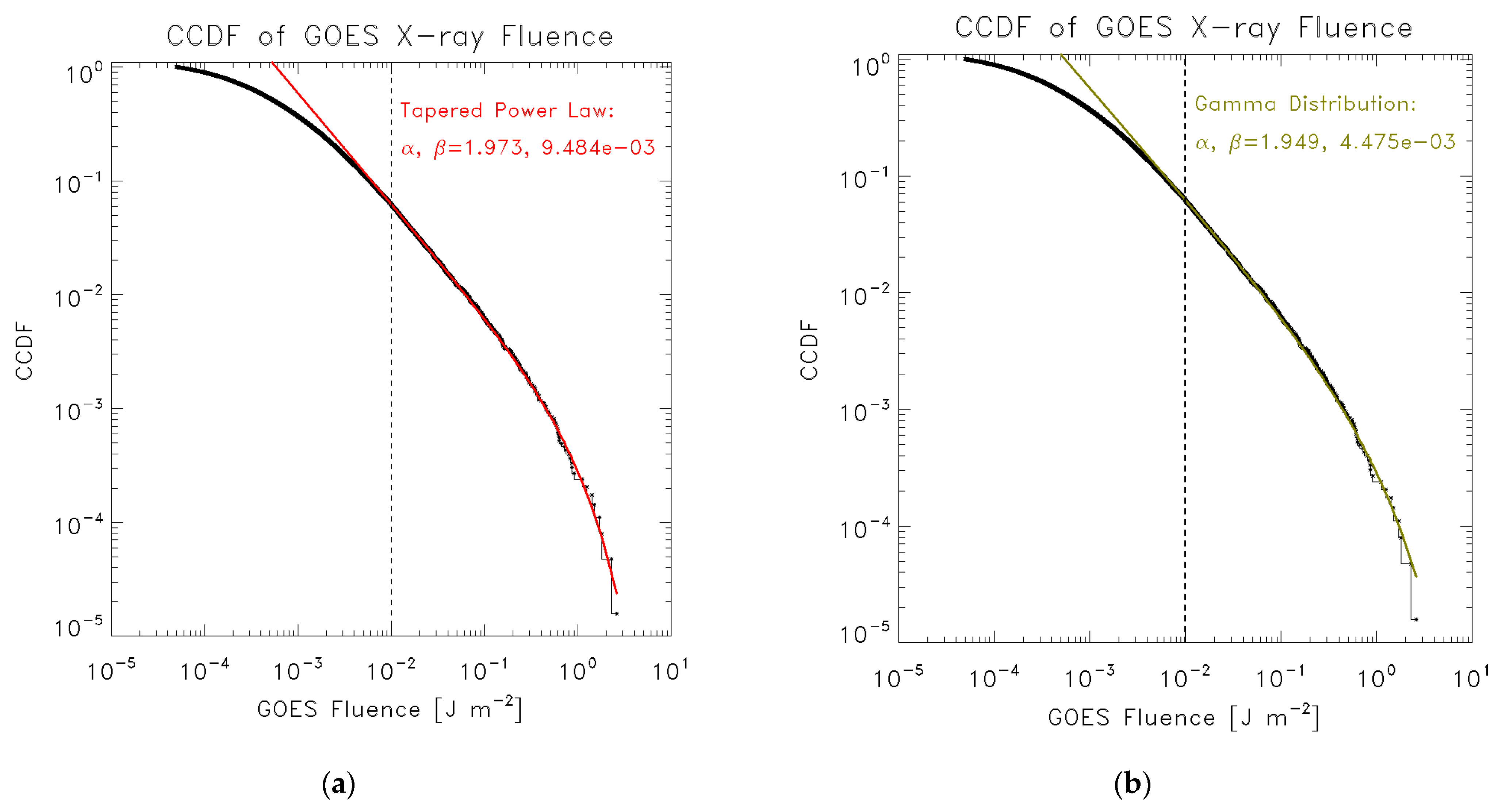
These two models (Figure 4a,b) show similar performance in terms of ΔAIC. The power-law indices α for the fluence are 1.973 for the tapered power law model and 1.949 for the gamma function model. Considering one-sigma errors one can still say that the values of α are less than 2, namely the total energy of all the flare populations is contributed primarily from large events. The values of α for the peak flux are 2.077 for the tapered power law model and 2.040 for the gamma function model, larger than 2. These values generally agree with the results of Ref. [17].
3.2. Weibull Distribution
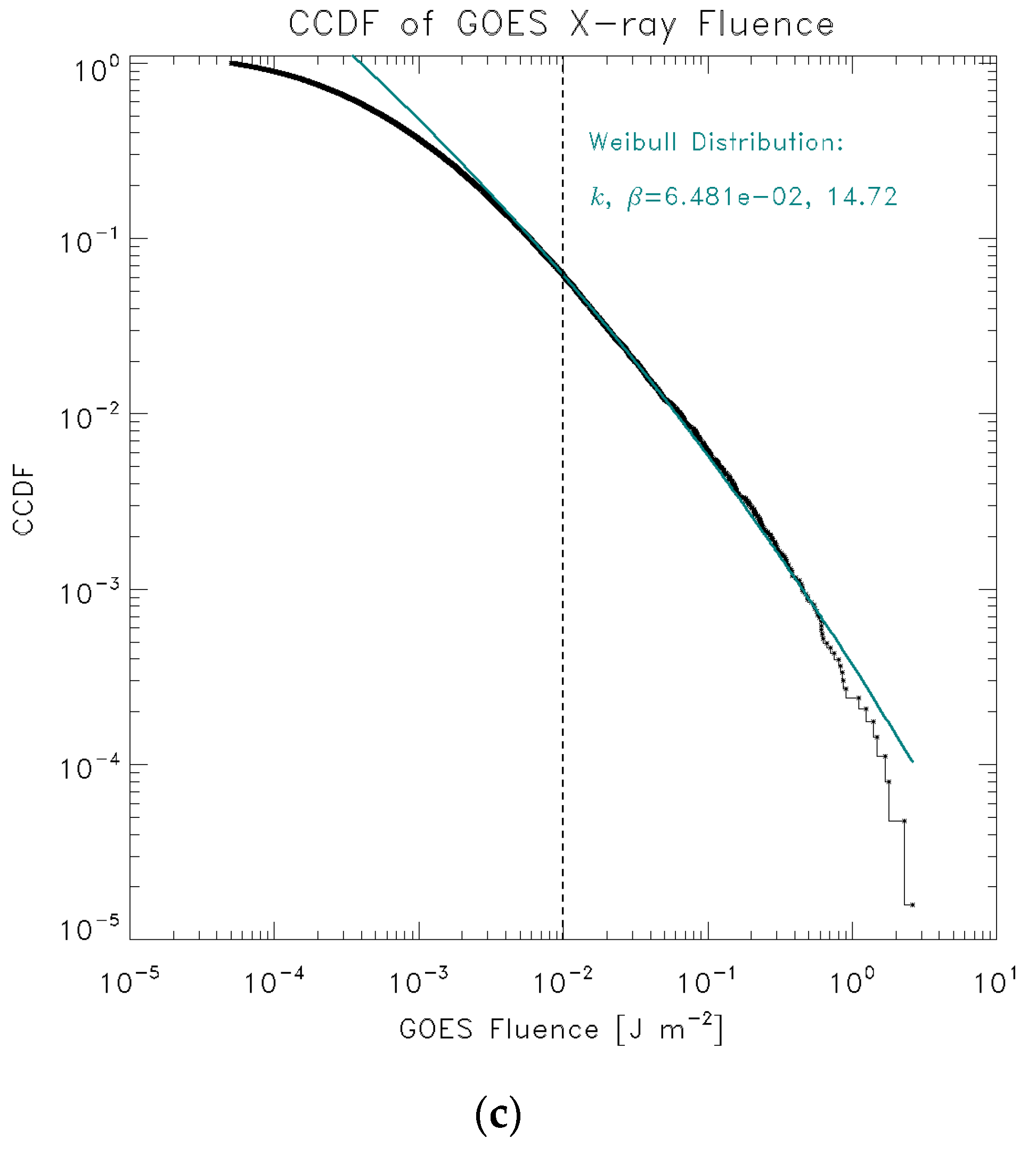
In terms of ΔAIC, the Weibull distribution (Figure 4c) cannot be dismissed but is supported only marginally (30 times less likely than the ΔAIC = 0 model).
If the distribution is extended to F << F0, the Weibull PDF approaches a power law with exponent 1 − k. Therefore, the fluence PDF behaves like F−(1−k) = F−0.935, which is significantly flatter than the tapered power law and gamma function distributions. This is another reason why the Weibull distribution is not favored compared to the tapered power law and gamma function distributions.
3.3. Comparison with Published Results
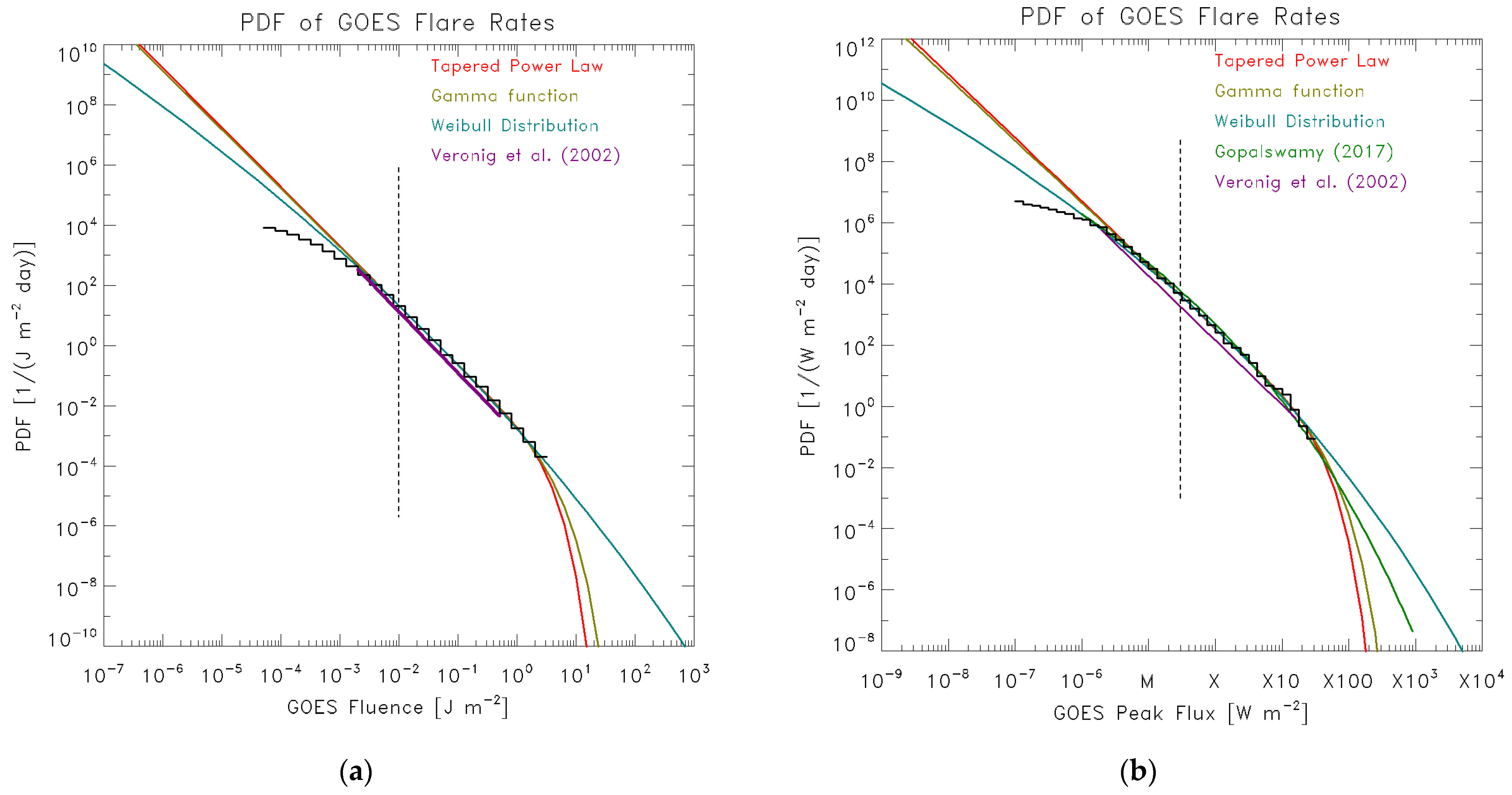
Similar analyses have been made by Veronig et al. [17] using the power law model and by Gopalswamy [33] using the Weibull function model. Figure 5 compares the present results with these publications. The tapered power law and gamma function distributions derived here show similar behaviors. The power-law distributions derived in Ref. [17] roughly follow the data histograms found here but deviates from the data at the higher end of the data. The Weibull distributions (both here and in Ref. [33]) become flatter at the smaller ends and decay less at the higher ends.
In the next Section, only the gamma function distributions are considered. The Weibull distributions are less favorable as described before. The tapered power-law PDFs are made of a mixture of two power-law exponents α and α − 1, and this sometimes may lead to undesirable features [30].
3.4. Prediction of Extreme Events
Based on the found fit to the flare fluence data in terms of the gamma function distribution, let us estimate the expected rates of large flares. The total soft X-ray energy emitted, EX, is given in terms of the X-ray flare fluence, F, as
Here, F is in J m−2, EX is in erg, and 1 astronomical unit (au) = 1.5 × 10¹¹ m. From this, Erad, the total radiated energy all over the electromagnetic spectrum (contributed mostly from ultra-violet (UV)) in erg, is estimated as [34]
The flare total (kinetic plus radiative) energy is approximately 4 times this quantity [34,35]. Finally, the quantities derived from the flare fluence data can be translated into the flare peak flux, Fp (J m−2), approximately by
which is the relation derived from our data.
EX = 2π × (1 au)2 × F × 107.
Erad = 1.03 × 10⁹ × EX0.766.
Fp ≈ 7.93 × 10⁻⁴ × F0.945,
Using these relations, the probability distribution function obtained here for soft X-ray fluence is translated to flare peak flux and total flare energy as shown in Table 3 and Table 4. Table 3 gives, for a specified value of flare fluence, the approximate peak flux, energy, and interval of flares exceeding the specified fluence. Table 4 gives, for a specified interval of a flare, the flare fluence, peak flux, and energy. The numbers are based on the gamma function distribution of α = 1.949, β = 0.00448. The second numbers after a slash are derived by assuming one-sigma errors (α = 1.949 + 0.021, β = 0.00448 − 0.0010 because the errors are correlated).
From Table 3, the Carrington event in 1 September 1859, which is estimated to be an X45 flare [34], may take place every 460 years, or every 110 years within one-sigma errors in α and β. From Table 4, the largest flare in 1000 years would be X46, or X69 (or X70 as a round number) for one-sigma errors. Even for the age of the solar system (4.6 × 10⁹ years), the largest flare we experience would be X224, or X374 for one-sigma errors.
4. Discussion
Recent discovery of energetic flares (called superflares) on solar-type stars observed with the Kepler satellite [36] (whose main targets are exoplanets, by high-precision photometry to detect the brightness decrease due to the transit of planets) has attracted attention in relation to extreme events that might happen on our Sun [13,14,37,38]. Those stellar flares are observed in the visible light; in the case of solar flares the emission in the visible light is detected only from intense flares (called “white-light flares”) [1].
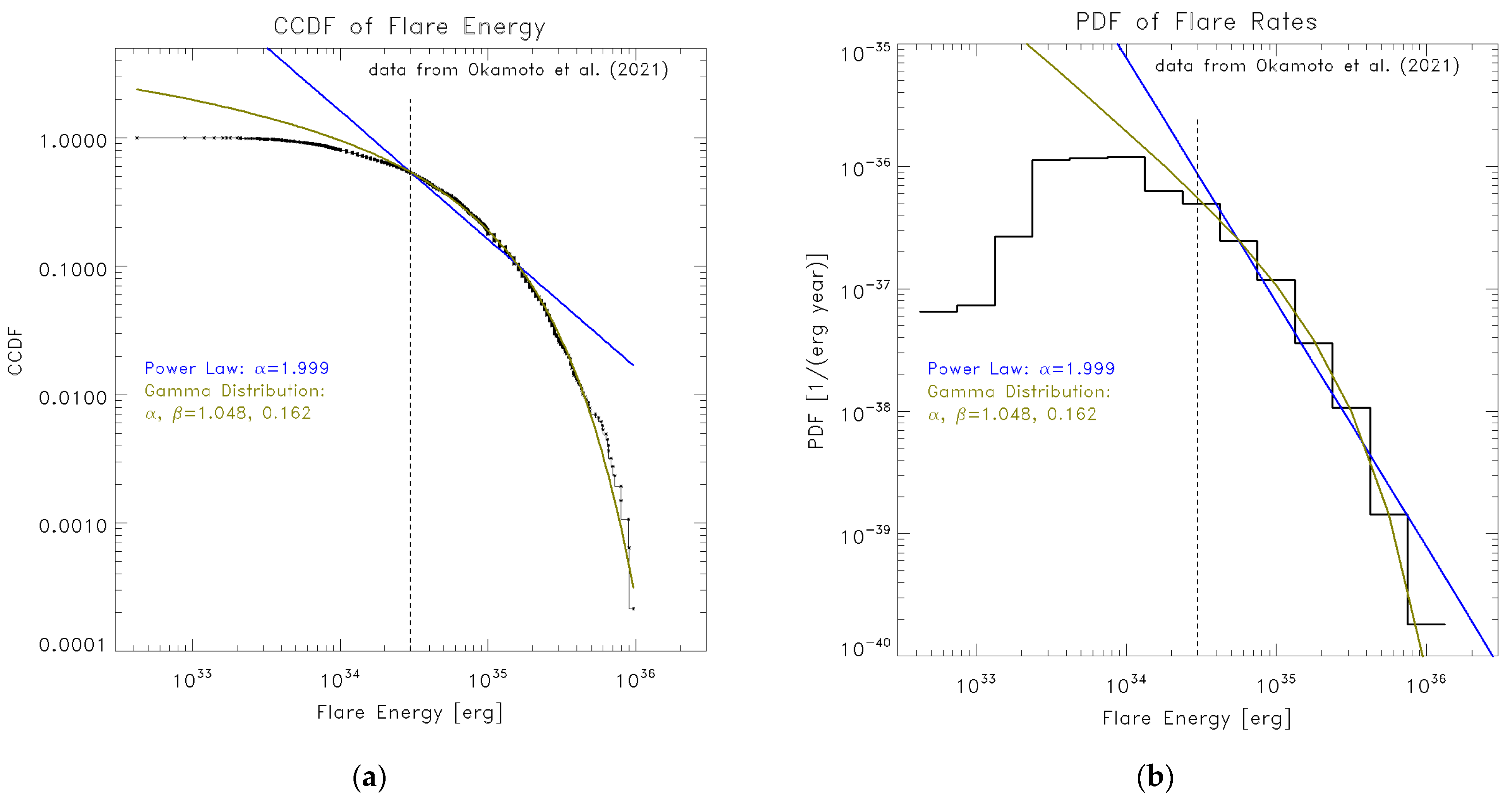
As an application of the analysis methods described in this paper, the energy distribution functions of stellar flares were studied. By using the most recent database on superflares from solar-type stars (G-type main-sequence stars with effective temperature of 5600−6000 K and rotation period longer than 20 days) which carefully removed contaminations from binaries or evolved stars [39], the results for CCDF and PDF have been obtained as shown in Figure 6a and Figure 6b, respectively. The data contain 2341 flares from 265 stars observed over 4 years. Both power law (blue) and gamma function (olive) model fits are shown. Here, the assumption is that the observed distribution function may mimic a hypothetical distribution function of flares from a single Sun-like star observed over 4 × 265 = 1060 years.
The value of ΔAIC of the power law model is about 90 compared to the gamma function distribution, so that the power law is unfavorable compared to the gamma function distribution. The power-law model gives a K-S measure √N × KS = 4.2 and its p-value is infinitesimally small. The gamma function model gives the parameter values α = 1.05, β = 0.16. The p-value from the K-S test is 0.39 and not so high, indicating room for better model of distribution functions.
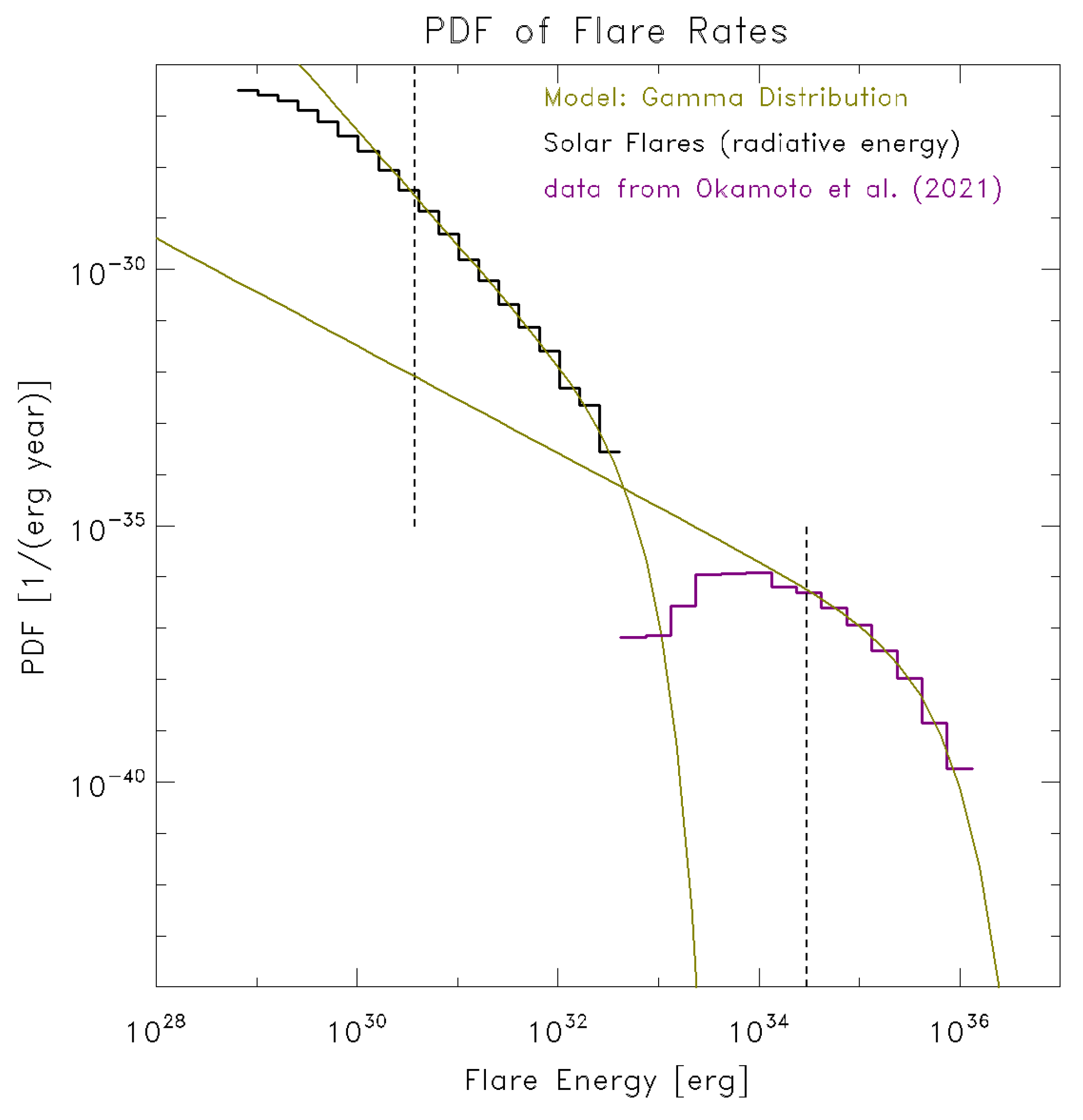
Combining the results shown in Figure 6 with those from Figure 4b, after converting flare fluence to radiated energy in the latter, Figure 7 is obtained. The F0 value of the GOES flare fluence, F0 = 1 × 10⁻² J m−2, is translated to the radiated energy of 3.8 × 1030 erg. It can be well seen that the PDF of solar flares does not connect to the stellar flare PDF but decays at an energy of approximately 1033.5 erg. Likewise, the PDF of stellar flares has a flatter distribution and does not connect to the PDF of solar flares. Although solar and stellar flares are both believed to be powered by magnetic energy (most likely by magnetic reconnection) of spotted regions, the distributions of the size and magnetic field strength in starspots would not be the same as in sunspots and may have a wider variety, because of different internal structures and rotation periods. Stellar flares may have a variety of power-exponent values, and the present results of α = 1.95 for solar flares and α = 1.05 for stellar flares are just two examples and there might be a continuous distribution of α between 1 and 2.
These results depend on the assumed values of the lower boundary of data for fitting. Ref. [19] proposes that the value of the lower boundary may also be selected by minimizing the K-S metric, but it seems that no consensus has been obtained yet [40,41]. In cases studied here, the turning down of the distributions toward smaller flares is due to the detection limits; small solar flares are not recognized as flares when the background level rises in the activity maximum period of the Sun’s eleven-year activity cycle. In the case of stellar flares, weak flares in more distant stars may be missed. On the other hand, if the boundary is set to a very large value, we will be left with only a small number of samples. The present approach is to find a compromise so that the samples are well above the detection limit and still a large number of samples is retained. It is desirable that more subjective methods are developed. It may also be useful to analyze data on flares from individual stars rather than using a composite data of many stars as used in this study.
5. Conclusions
From the analysis of soft X-ray data of the GOES satellites, in this paper, it is found that the distribution functions of solar flare fluence are successfully modeled by tapered power law or gamma function distributions whose power exponent is slightly smaller than 2, indicating that the total energy of the flare populations is mostly contributed from a small number of large flares. The tapering off of the distribution is statistically significant and the power law fit is rejected. The largest possible flares in 1000 years are predicted to be around X46, or X69 for one-sigma errors in the derived parameters. The upper limits of X224 (X374 for one-sigma errors) are derived even by considering the lifetime of the solar system.
Similar treatment was applied to flares from solar-type stars. They were fitted by a gamma function distribution (the power law is rejected), but their power exponent is around 1.05, which is smaller than the solar flare case (around 1.95). Therefore, the stellar flare data analyzed here do not connect to the energy distribution function of solar flares. It would be interesting to see how the distribution functions differ among solar-type stars with different effective temperatures and rotation periods.
Supplementary Materials
The data sets used in the present analysis are available at http://solarwww.mtk.nao.ac.jp/sakurai/tar/goesfluence_datalist.zip (accessed on 10 December 2022), http://solarwww.mtk.nao.ac.jp/sakurai/tar/goesflux_datalist.zip (accessed on 10 December 2022), for the flare fluence above 5 × 10⁻⁵ J m−2 (1997–2020) and peak flux above 1 × 10⁻⁷ W m−2 (1980–2020), respectively.
Funding
This research was supported by the Japan Society for the Promotion of Science (JSPS) KAKENHI Grant numbers JP15H05816 and JP20K04033.
Data Availability Statement
The GOES flare peak flux data are available at https://www.ngdc.noaa.gov/stp/space-weather/solar-data/solar-features/solar-flares/x-rays/goes/xrs/ (accessed on 10 December 2022) for the years 1975–2016 and at tftp://ftp.swpc.noaa.gov/pub/warehouse/ (accessed on 10 December 2022) for 2017 and later. The fluence data are included in these data after 1997. The X-ray background data for the years 1983–2011 are given in ftp://ftp.ngdc.noaa.gov/STP/SOLAR_DATA/SATELLITE_ENVIRONMENT/Daily_Fluences/Fluence (accessed on 10 December 2022). The background data for 2011–2019 are available at https://satdat.ngdc.noaa.gov/sem/goes/data/science/xrs/ (accessed on 10 December 2022) and at https://data.ngdc.noaa.gov/platforms/solar-space-observing-satellites/goes/ (accessed on 10 December 2022) for 2020. The background values between 1983 March and 1987 were calculated from the 1 min intensities given at https://satdat.ngdc.noaa.gov/sem/goes/data/avg (accessed on 10 December 2022). The data on stellar flares discussed in Section 4 are provided in Ref. [39] and are available at https://cfn-live-content-bucket-iop-org.s3.amazonaws.com/journals/0004-637X/906/2/72/revision1/apjabc8f5t2_mrt.txt?AWSAccessKeyId=AKIAYDKQL6LTV7YY2HIK&Expires=1672409945&Signature=9PZI1nNLGpdBDh043SiGsSXeAuQ%3D (accessed on 10 December 2022).
Acknowledgments
The author would like to thank Shin Toriumi for discussion. It is a great pleasure for the author to express appreciations to Marcel Goossens for his hospitality during the author’s visit to Katholieke Universiteit Leuven in 1989 that led to a couple of jointly written papers.
Conflicts of Interest
The author declares no conflict of interest.
References
- Švestka, Ž. Solar Flares; D. Reidel Publishing Company: Dordrecht, The Netherlands, 1976. [Google Scholar] [CrossRef]
- Benz, A.O. Flare observations. Living Rev. Sol. Phys. 2017, 14, 2. [Google Scholar] [CrossRef] [Green Version]
- Carrington, R.C. Description of a singular appearance seen in the Sun on September 1, 1859. Mon. Not. R. Astron. Soc. 1859, 20, 13–15. [Google Scholar] [CrossRef] [Green Version]
- Cliver, E.W.; Schrijver, C.J.; Shibata, K.; Usoskin, I.G. Extreme solar events. Living Rev. Sol. Phys. 2022, 19, 2. [Google Scholar] [CrossRef]
- Priest, E.R.; Forbes, T.G. The magnetic nature of solar flares. Astron. Astrophys. Rev. 2002, 10, 313–377. [Google Scholar] [CrossRef]
- Lin, R.P.; Schwartz, R.A.; Kane, S.R.; Pelling, R.M.; Hurley, K.C. Solar hard X-ray microflares. Astrophys. J. 1984, 283, 421–425. [Google Scholar] [CrossRef]
- Crosby, N.; Aschwanden, M.; Dennis, B. Frequency distributions and correlations of solar X-ray flare parameters. Sol. Phys. 1993, 143, 275–299. [Google Scholar] [CrossRef]
- Parker, E.N. Nanoflares and the solar X-ray corona. Astrophys. J. 1988, 330, 474–479. [Google Scholar] [CrossRef]
- Sakurai, T. Heating mechanisms of the solar corona. Proc. Jpn. Acad. Ser. B 2017, 93, 87–97. [Google Scholar] [CrossRef] [Green Version]
- McIntosh, S.W.; de Pontieu, B.; Carlsson, M.; Hansteen, V.; Boerner, P.; Goossens, M. Alfvénic waves with sufficient energy to power the quiet solar corona and fast solar wind. Nature 2011, 475, 477–480. [Google Scholar] [CrossRef]
- Hinode Review Team. Achievements of Hinode in the first eleven years. Publ. Astron. Soc. Jpn. 2019, 71, R1. [Google Scholar] [CrossRef] [Green Version]
- Hudson, H.S. Solar flares, microflares, nanoflares, and coronal heating. Sol. Phys. 1991, 133, 357–369. [Google Scholar] [CrossRef]
- Schaefer, B.E.; King, J.R.; Deliyannis, C.P. Superflares on ordinary solar-type stars. Astrophys. J. 2000, 529, 1026–1030. [Google Scholar] [CrossRef] [Green Version]
- Maehara, H.; Shibayama, T.; Notsu, S.; Notsu, Y.; Nagao, T.; Kusaba, S.; Honda, S.; Nogami, D.; Shibata, K. Superflares on solar-type stars. Nature 2012, 485, 478–481. [Google Scholar] [CrossRef] [PubMed]
- Machol, J.; Viereck, R.; Peck, C.; Mothersbaugh, J., III. GOES X-ray Sensor (XRS) Operational Data; NOAA National Centers for Environmental Information (NCEI): Boulder, CO, USA, 2022. Available online: https://www.ngdc.noaa.gov/stp/satellite/goes/doc/GOES_XRS_readme.pdf (accessed on 10 December 2022).
- Bornmann, P.L.; Speich, D.; Hirman, J.; Matheson, L.; Grubb, R.; Garcia, H.A.; Viereck, R. GOES X-ray sensor and its use in predicting solar-terrestrial disturbances. In GOES-8 and Beyond. Proceedings of SPIE, Vol. 2812; Washwell, E.R., Ed.; Society of Photo-Optical Instrumentation Engineers (SPIE): Bellingham, WA, USA, 1996; pp. 291–298. [Google Scholar] [CrossRef]
- Veronig, A.; Temmer, M.; Hanslmeier, A.; Oruba, W.; Messerotti, M. Temporal aspects and frequency distributions of solar soft X-ray flares. Astron. Astrophys. 2002, 382, 1070–1080. [Google Scholar] [CrossRef] [Green Version]
- Donnelly, R.F. Solar flare X-ray and EUV emission: A terrestrial viewpoint. In Physics of Solar Planetary Environments; Williams, D.J., Ed.; American Geophysical Union: Washington, DC, USA, 1976; Volume 1, pp. 178–192. [Google Scholar] [CrossRef]
- Clauset, A.; Shalizi, C.R.; Newman, M.E.J. Power-law distributions in empirical data. SIAM Rev. 2009, 51, 661–703. [Google Scholar] [CrossRef] [Green Version]
- Kagan, Y.Y. Seismic moment distribution revisited: I. Statistical results. Geophys. J. Int. 2002, 148, 520–541. [Google Scholar] [CrossRef] [Green Version]
- Kagan, Y.Y. Seismic moment distributions. Geophys. J. Int. 1991, 106, 123–134. [Google Scholar] [CrossRef]
- Gutenberg, B.; Richter, C.F. Earthquake magnitude, intensity, energy, and acceleration. Bull. Seismol. Soc. Am. 1942, 32, 163–191. [Google Scholar] [CrossRef]
- Utsu, T. Representation and analysis of the earthquake size distribution: A historical review and some new approaches. Pure Appl. Geophys. 1999, 155, 509–535. [Google Scholar] [CrossRef]
- Weibull, W. The Phenomenon of Rupture in Solids. R. Swed. Inst. Engineer. Res. Proceed. 1939, 153, 1–55. Available online: https://pdfcoffee.com//the-phenomenon-of-rupture-in-solids-weibull-1939-pdf-free.html (accessed on 10 December 2022).
- Vere-Jones, D.; Robinson, R.; Yang, W. Remarks on the accelerated moment release model: Problems of model formulation, simulation and estimation. Geophys. J. Int. 2001, 144, 517–531. [Google Scholar] [CrossRef] [Green Version]
- Wingo, D.R. The left-truncated Weibull distribution: Theory and computation. Stat. Pap. 1989, 30, 39–48. [Google Scholar] [CrossRef]
- Stephens, M.A. EDF statistics for goodness of fit and some comparisons. J. Am. Stat. Assoc. 1974, 69, 730–737. [Google Scholar] [CrossRef]
- Akaike, H. A new look at the statistical model identification. IEEE Trans. Automat. Control 1974, 19, 716–723. [Google Scholar] [CrossRef]
- Burnham, K.P.; Anderson, D.R.; Huyvaert, K.P. AIC model selection and multimodel inference in behavioral ecology: Some background, observations, and comparisons. Behav. Ecol. Sociobiol. 2011, 65, 23–35. [Google Scholar] [CrossRef]
- Sakurai, T.; Toriumi, S. Probability distribution functions of sunspot magnetic flux. arXiv 2022, arXiv:2211.13957. [Google Scholar] [CrossRef]
- Efron, B.; Tobshirani, R.J. An Introduction to the Bootstrap; Springer Science+Business Media: Dordrecht, The Netherlands, 1993; pp. 53–56. [Google Scholar]
- Simard, R.; L’Ecuyer, P. Computing the Two-Sided Kolmogorov-Smirnov Distribution. J. Stat. Softw. 2011, 39, 1–18. [Google Scholar] [CrossRef] [Green Version]
- Gopalswamy, N. Extreme solar eruptions and their space weather consequences. In Extreme Events in Geospace; Buzulukova, N., Ed.; Elsevier: Amsterdam, The Netherlands, 2018; pp. 37–63. [Google Scholar] [CrossRef]
- Cliver, E.W.; Dietrich, W.F. The 1859 space weather event revisited: Limits of extreme activity. J. Space Weather Space Clim. 2013, 3, A31. [Google Scholar] [CrossRef] [Green Version]
- Emslie, A.G.; Dennis, B.R.; Shih, A.Y.; Chamberlin, P.C.; Mewaldt, R.A.; Moore, C.S.; Share, H.; Vourlidas, A.; Welsch, B.T. Global energetics of thirty-eight large solar eruptive events. Astrophys. J. 2012, 759, 71. [Google Scholar] [CrossRef] [Green Version]
- Koch, D.G.; Borucki, W.J.; Basri, G.; Batalha, N.M.; Brown, T.M.; Caldwell, D.; Christensen-Dalsgaard, J.; Cochran, W.D.; DeVore, E.; Dunham, E.W.; et al. Kepler mission—Design, realized photometric performance, and early science. Astrophys. J. Lett. 2010, 713, L79–L86. [Google Scholar] [CrossRef] [Green Version]
- Shibayama, T.; Maehara, H.; Notsu, S.; Notsu, Y.; Nagao, T.; Honda, S.; Ishii, T.; Nogami, D.; Shibata, K. Superflares on solar-type stars observed with Kepler. I. Statistical properties of superflares. Astrophys. J. Suppl. 2013, 209, 5. [Google Scholar] [CrossRef] [Green Version]
- Maehara, H.; Shibayama, T.; Notsu, Y.; Notsu, S.; Honda, S.; Nogami, D.; Shibata, K. Statistical properties of superflares on solar-type stars based on 1-min cadence data. Earth Planets Space 2015, 67, 59. [Google Scholar] [CrossRef] [Green Version]
- Okamoto, S.; Notsu, Y.; Maehara, H.; Namekata, K.; Honda, S.; Ikuta, K.; Nogami, D.; Shibata, K. Statistical properties of superflares on solar-type stars: Results using all of the Kepler primary mission data. Astrophys. J. 2021, 906, 72. [Google Scholar] [CrossRef]
- Deluca, A.; Corral, Á. Fitting and goodness-of-fit test of non-truncated and truncated power-law distributions. Acta Geophys. 2013, 61, 1351–1394. [Google Scholar] [CrossRef] [Green Version]
- Corral, Á.; Gonzalez, Á. Power law size distributions in geoscience revisited. Earth Space Sci. 2019, 6, 673–697. [Google Scholar] [CrossRef]
Figure 1.
Solar soft X-ray flares detected by the Geostationary Operational Environmental Satellites (GOES): peak flux (a) and fluence of flares (b) as a function of year.
Figure 1.
Solar soft X-ray flares detected by the Geostationary Operational Environmental Satellites (GOES): peak flux (a) and fluence of flares (b) as a function of year.

Figure 2.
Complementary cumulative distribution function (a) and occurrence rates (b) of flare fluence, F. The histogram in plot (b) is built with a bin-size of Δlog10F = 0.2. Short vertical bars indicate statistical errors of √n on the bins with counts n.
Figure 2.
Complementary cumulative distribution function (a) and occurrence rates (b) of flare fluence, F. The histogram in plot (b) is built with a bin-size of Δlog10F = 0.2. Short vertical bars indicate statistical errors of √n on the bins with counts n.

Figure 3.
(a) The blue line shows the power-law fit to the observed CCDF of GOES flare fluence data. (b) The derived power-law distribution overplotted on the observed flare occurrence rate histogram. The vertical dashed line indicates the lower boundary (1 × 10⁻² J m−2) of data used for fitting.
Figure 3.
(a) The blue line shows the power-law fit to the observed CCDF of GOES flare fluence data. (b) The derived power-law distribution overplotted on the observed flare occurrence rate histogram. The vertical dashed line indicates the lower boundary (1 × 10⁻² J m−2) of data used for fitting.

Figure 4.
The CCDFs of flare fluence data fitted by (a) a tapered power law, (b) a gamma function distribution, and (c) a Weibull distribution. The vertical dashed line indicates the lower boundary (1 × 10⁻² J m−2) of data used for fitting.
Figure 4.
The CCDFs of flare fluence data fitted by (a) a tapered power law, (b) a gamma function distribution, and (c) a Weibull distribution. The vertical dashed line indicates the lower boundary (1 × 10⁻² J m−2) of data used for fitting.


Figure 5.
This analysis results compared to earlier findings [17,33] of the flare occurrence rates (PDFs) for fluence (a) and peak flux (b). The thick black histograms are the observed PDFs. Red, olive, and teal curves indicate, respectively, tapered power law, gamma function, and Weibull distributions fitted to the data. Purple and green curves are power law [17] and Weibull [33] fits, respectively. The vertical dashed lines indicate the lower boundary in the data used for fitting, namely 1 × 10⁻² J m−2 for fluence and M3 (3 × 10⁻⁵ W m−2) for peak flux, respectively. Veronig et al.’s [17] parameters of power-law fits are: N = 8400, τobs = 4 years, α = 2.03, and F0 = 2 × 10⁻³ J m−2 (for flare fluence), and Np = 49409, τobs,p = 25 years, F0p = 2 × 10⁻⁶ W m−2, and α = 2.11 (for flare peak flux). Gopalswamy’s [33] parameters of Weibull distribution fit are: Np = 55285, τobs,p = 48 years, F0p = 9.1 × 10⁻⁷ W m−2, k = 0.167, and β = 3.77. See text for details.

Figure 6.
Statistical distributions of flares on solar-type stars. (a) CCDF with a power-law (blue) and gamma function (olive) distribution fits. (b) The histogram of flare occurrence rates with the derived power law and gamma function distributions. The data are from [39]. The vertical dashed line indicates the lower boundary (3 × 1034 erg) of the data used for fitting.

Figure 7.
Comparison of solar and stellar flare energy distributions. Black and purple histograms show the occurrence rates of solar X-ray flares and stellar flares [39], respectively. The olive curves are fit to these data by the gamma function distributions. The vertical dashed lines indicate the lower boundary for fitting adopted for the solar flare data (3.8 × 1030 erg of radiated energy) and for the stellar flare data (3 × 1034 erg).


Table 1.
Derived parameters for X-ray fluence distributions (F0 = 1 × 10⁻² J m−2, N = 1945). See text for details.
Table 1.
Derived parameters for X-ray fluence distributions (F0 = 1 × 10⁻² J m−2, N = 1945). See text for details.
| Model | α | β | ΔAIC | √N × KS | K-S p-Value |
|---|---|---|---|---|---|
| Power law | 2.015 ± 0.023 | 11.6 | 0.69 | 0.72 | |
| Tapered power law | 1.973 ± 0.021 | 0.00948 ± 0.0031 | 0.00 | 0.47 | 0.98 |
| Gamma function | 1.949 ± 0.032 | 0.00448 ± 0.0020 | 1.10 | 0.57 | 0.90 |
| Weibull | k = 0.0648 ± 0.0242 | 14.7 ± 5.9 | 7.20 | 0.69 | 0.73 |
Table 2.
Derived parameters for X-ray peak flux distributions (F0p = 3 × 10⁻⁵ W m−2, N = 1720). See text for details.
Table 2.
Derived parameters for X-ray peak flux distributions (F0p = 3 × 10⁻⁵ W m−2, N = 1720). See text for details.
| Model | α | β | ΔAIC | √N × KS | K-S p-Value |
|---|---|---|---|---|---|
| Power law | 2.162 ± 0.028 | 15.7 | 0.89 | 0.41 | |
| Tapered power law | 2.077 ± 0.032 | 0.026 ± 0.007 | 0.00 | 0.40 | 0.99 |
| Gamma function | 2.040 ± 0.045 | 0.014 ± 0.005 | 1.48 | 0.44 | 0.99 |
| Weibull | k = 0.104 ± 0.030 | 10.2 ± 3.3 | 7.00 | 0.57 | 0.90 |
Table 3.
Predicted flare intervals as a function of X-ray fluence values (gamma function distribution, α = 1.949 ± 0.032, β = 0.00448 ± 0.0020). The second numbers after a slash are derived by assuming one-sigma errors (α = 1.949 + 0.032, β = 0.00448 − 0.0020). See text for details.
Table 3.
Predicted flare intervals as a function of X-ray fluence values (gamma function distribution, α = 1.949 ± 0.032, β = 0.00448 ± 0.0020). The second numbers after a slash are derived by assuming one-sigma errors (α = 1.949 + 0.032, β = 0.00448 − 0.0020). See text for details.
| X-ray Fluence (J m−2) | Approx. GOES Flux | Total Energy (erg) | Interval (Years) |
|---|---|---|---|
| 1.0 × 10⁻² | M1.0 | 1.5 × 1031 | 1.3 × 10⁻²/1.3 × 10−2 |
| 1.0 × 10⁻¹ | M9.0 | 8.8 × 1031 | 1.4 × 10⁻¹/1.4 × 10−1 |
| 1.0 × 100 | X7 | 5.1 × 1032 | 3.0 × 100/2.3 × 100 |
| 2.0 × 100 | X15 | 8.7 × 1032 | 1.2 × 101/7.3 × 100 |
| 5.0 × 100 | X36 | 1.8 × 1033 | 1.8 × 10²/5.6 × 101 |
| 6.3 × 100 | X45 † | 2.1 × 1033 | 4.6 × 10²/1.1 × 102 |
† Carrington event (1859 Sept.1) [34].
Table 4.
Predicted flare sizes as a function of flare intervals (gamma function distribution, α = 1.949 ± 0.032, β = 0.00448 ± 0.0020). The second numbers after a slash are derived by assuming one-sigma errors (α = 1.949 + 0.032, β = 0.00448 − 0.0020). See text for details.
Table 4.
Predicted flare sizes as a function of flare intervals (gamma function distribution, α = 1.949 ± 0.032, β = 0.00448 ± 0.0020). The second numbers after a slash are derived by assuming one-sigma errors (α = 1.949 + 0.032, β = 0.00448 − 0.0020). See text for details.
| X-ray Fluence (J m−2) | Approx. GOES Flux | Total Energy (erg) | Interval (Years) |
|---|---|---|---|
| 6.5 × 100/9.9 × 100 | X46/X69 | 2.2 × 1033/3.0 × 1033 | 1.0 × 10³ |
| 1.0 × 101/1.6 × 101 | X70/X108 | 3.0 × 1033/4.3 × 1033 | 1.0 × 10⁴ |
| 1.4 × 101/2.3 × 101 | X95/X152 | 3.8 × 1033/5.6 × 1033 | 1.0 × 10⁵ |
| 1.8 × 101/3.0 × 101 | X122/X197 | 4.7 × 1033/6.9 × 1033 | 1.0 × 10⁶ |
| 2.7 × 101/4.6 × 101 | X177/X293 | 6.3 × 1033/9.5 × 1033 | 1.0 × 10⁸ |
| 3.4 × 101/5.9 × 101 | X224/X374 | 7.7 × 1033/1.2 × 1034 | 4.6 × 10⁹ |
Disclaimer/Publisher’s Note: The statements, opinions and data contained in all publications are solely those of the individual author(s) and contributor(s) and not of MDPI and/or the editor(s). MDPI and/or the editor(s) disclaim responsibility for any injury to people or property resulting from any ideas, methods, instructions or products referred to in the content. |
© 2022 by the author. Licensee MDPI, Basel, Switzerland. This article is an open access article distributed under the terms and conditions of the Creative Commons Attribution (CC BY) license (https://creativecommons.org/licenses/by/4.0/).
Share and Cite
MDPI and ACS Style
Sakurai, T. Probability Distribution Functions of Solar and Stellar Flares. Physics 2023, 5, 11-23. https://doi.org/10.3390/physics5010002
AMA Style
Sakurai T. Probability Distribution Functions of Solar and Stellar Flares. Physics. 2023; 5(1):11-23. https://doi.org/10.3390/physics5010002
Chicago/Turabian StyleSakurai, Takashi. 2023. "Probability Distribution Functions of Solar and Stellar Flares" Physics 5, no. 1: 11-23. https://doi.org/10.3390/physics5010002