A Chaotic Second Order Oscillation JAYA Algorithm for Parameter Extraction of Photovoltaic Models


School of Optical Electrical and Computer Engineering, University of Shanghai for Science and Technology, Shanghai 200093, China
*
Author to whom correspondence should be addressed.
Photonics 2022, 9(3), 131; https://doi.org/10.3390/photonics9030131
Submission received: 20 January 2022
/
Revised: 21 February 2022
/
Accepted: 22 February 2022
/
Published: 25 February 2022
(This article belongs to the Special Issue Advances in Photovoltaic Technologies from Atomic to Device Scale)
Abstract
:In order to identify the parameters of photovoltaic (PV) cells and modules more accurately, reliably and efficiently, a chaotic second order oscillation JAYA algorithm (CSOOJAYA) is proposed. Firstly, both logical chaotic map and the mutation strategy are brought in enhancing the population diversity and improving exploitation. Secondly, in order to better balance exploration and exploitation, the second order oscillation factor is added, which not only improves the diversity of the population, but also has strong exploration at the beginning of the iteration and strong exploitation at the end of the iteration. In order to balance the two abilities, the self-adaptive weight is introduced into the CSOOJAYA algorithm to regulate individuals the tendency of moving toward the optimal solution and escaping from the worst solution, so as to enhance the search efficiency and exploitation. In order to validate the behavior of CSOOJAYA, it is employed to the parameter identification problem of PV models. Finally, the experimental results show that CSOOJAYA delivers excellent behavior in the aspects of convergence, reliability and accuracy.
1. Introduction
In order to alleviate the greenhouse effect and solve problems such as global warming, the application of renewable energy has attracted much attention [1]. Among the renewable energy sources, solar energy is considered as one of the most promising renewable energy source because of its green, clean, widely distributed and free energy [2]. Solar PV systems can directly convert solar energy into electrical energy, so it has become one of the most widely used power generation technologies [3]. However, PV systems are susceptible to external factors, especially irradiance and temperature [4]. PV arrays tend to degrade over time under harsh environmental conditions, significantly affecting the behavior and utilization efficiency of PV systems [5]. Therefore, in order to accurately control PV systems, it is significant to adopt the experimentally measured current-voltage (I-V) data to estimate the actual behavior of PV systems at work [6]. The single diode model (SDM) and the double diode model (DDM) are widely employed and can accurately reflect the nonlinear behavior of PV panels [7]. The parameter accuracy of these models is essential for modeling, control and optimization of PV panels [8]. However, these parameters are susceptible to various environmental factors and become unavailable [9]. PV models are implicitly nonlinear transcendental equations [10]. It is very significant and challenging to employ an efficient and reliable methods to identify the PV parameters.
Many methods have been proposed to solve PV parameter identification. In principle, these methods can be divided into analytical methods and optimization methods [11]. The analytical methods mainly employ several key data (short-circuit current, open-circuit voltage, and maximum power) provided by the manufacturer, and use mathematical equations to deduce the parameters [12]. The analytical methods have the advantages of simple, fast and direct calculation. However, these data are obtained under standard test conditions [13]. Therefore, the extracted parameters above cannot precisely predict the I-V curves at different temperatures and solar irradiance [14]. Furthermore, this approach depends heavily on the key points of the selected I-V characteristics. If the crucial points are wrongly selected, the computational accuracy will be significantly reduced [11].
Instead of choosing a few key points, the optimization method takes into account all the actual measured current and voltage data. From the algorithm point of view, optimization methods can be divided into meta-heuristic methods and deterministic methods [15]. The optimization methods transform the PV parameter identification problem into an optimization problem, and then the parameters are identified according to all the reference points on the I-V characteristic curve. Deterministic methods, such as Newton–Raphson method [16,17], iterative curve fitting [18,19] and Lambert W-function [20,21], require the objective function to be continuous, convex, and differentiable [22]. The I-V curve of the PV cell model is non-linear, multi-peak and multi-mode. And the deterministic method is easily affected by the initial conditions and gradient information, so it is free to become trapped in a local optimum when resolving such complicated problems [23].
The heuristic methods have no strict requirements on the form of the optimization problem and are not affected by initial conditions and gradient information [24]. Therefore, many heuristic methods have been used to identify the parameters of PV models in the past ten years. These include the classified perturbation mutation based particle swarm optimization algorithm (CPMPSO) [1], efficient teaching-learning-based optimization algorithm (MTLBO) [16], multiswarm spiral leader particle swarm optimization algorithm (MSLPSO) [18], enhanced adaptive differential evolution algorithm (EJADE) [22], memetic adaptive differential evolution (MADE) [23], modified Rao-1 optimization algorithm (MRAO-1) [25], improved gaining-sharing knowledge algorithm (IGSK) [26] and chaos induced coyote algorithm (CICA) [27]. The characteristics of the three existing methods are summarized in Table 1.
Compared with deterministic methods, heuristic methods can acquire more precise and robust PV parameter identification results. However, PV models are nonlinear and multi-mode, so some heuristic methods may become trapped in local optima during the optimization process [8]. In addition to the basic parameters of population size and termination condition, most heuristic algorithms have specific parameters related to their own mechanisms. The behavior of the heuristic algorithm depends to some extent on these specific parameters. Choosing inappropriate parameters will not only increase the computational burden of the algorithm, but it may also converge prematurely or fall into a local optimum [28].
Rao proposed a new and efficient heuristic algorithm in 2016, namely the JAYA algorithm [29]. The structure of the JAYA algorithm is relatively simple, with only two parameters: population size and termination conditions [28]. Therefore, the advantage of the JAYA algorithm is that it can reduce the time of the optimization process and avoid the difficulties caused by parameter adjustment. However, the individual position is only affected by the current optimal individual and the worst individual in the JAYA algorithm, which cannot effectively maintain the diversity of the population [8]. Therefore, JAYA algorithm is free to trap in local optimum when solving complicated problems such as multi-peak and multi-mode.
Although the performance of some improved JAYA algorithms such as the performance-guided JAYA algorithm or PGJAYA [8], comprehensive learning JAYA algorithm (CLJAYA) [10], improved JAYA algorithm (IJAYA) [28], logistic chaotic JAYA algorithm (LCJAYA) [29], and elite opposition-based JAYA algorithm (EO-JAYA) [30] have been improved to some extent, the imbalance between exploration and exploitation is not fully considered. The corresponding summary of the extraction parameters of existing heuristic methods is shown in Table 2.
In order to improve the performance of JAYA algorithm, this paper proposes a chaotic second order oscillation JAYA algorithm (CSOOJAYA), which can identify parameters more accurately and stably. Firstly, the introduction of logical chaotic mapping mechanism improves the population diversity and exploration. Secondly, the introduction of the second order oscillation mechanism not only improves the diversity of the population, but also has strong exploration ability due to the oscillation convergence of the solution vector in the early iteration. The solution vector converges asymptotically in the later iteration and has strong exploitation ability. The self-adaptive weight mechanism is introduced to adjust the tendency of individuals to approach the optimal solution and escape the worst solution, improve the search efficiency of the population and the exploitation. The algorithm improves and balances the global search ability and local optimization ability as a whole. The introduction of mutation mechanisms ensures that individuals avoid getting stuck in local optima. The structure of CSOOJAYA is similar to the JAYA algorithm, and it only has two parameters: population size and termination condition. In order to verify the effectiveness of the proposed CSOOJAYA algorithm, CSOOJAYA and other novel algorithms are used to extract the parameters of three PV models. The experimental results show that CSOOJAYA has the best performance in terms of identification accuracy, stability and convergence speed.
2. PV Models and Objective Function
2.1. Formula of SDM
Figure 1 presents the circuit diagram of the SDM. Obviously, the framework of the SDM is relatively simple. There are photogenerated current , output current , diode current , and shunt current in the circuit. According to Kirchhoff current law, can be get by Equation (1). According to the diode Shockley equation and Ohm law, can be get by Equation (2), and can be obtained by Equation (3):
refers to the series resistance, stands for the parallel resistance, stands for the output voltage, n is the ideality factor of the diode. k refers to the Boltzmann constant (1.3806503 × J/K), q stands for the elementary charge (1.60217646 × C), and T refers to the absolute temperature. Therefore, we can substitute Equations (2) and (3) into Equation (1) to get Equation (4).
Obviously, SDM needs to identify five unknown different parameters (, , , , n).
2.2. Formula of DDM
Taking into account the inherent drawbacks of SDM, DDM can more accurately illustrate the relationship between voltage and current. Figure 2 presents the circuit diagram of the DDM. It can be seen from the Figure 2, DDM differs from SDM in that it has one more diode in parallel with the current source than SDM. can be obtained by Equation (5):
refers to the diode diffusion current, and stands for the saturation current. and represent the ideal saturation factor of two diodes, respectively. Obviously, the DDM needs to extract seven unknown different parameters (, , , , , , ).
2.3. Formula of PV Module
Figure 3 presents the circuit diagram of a PV module, which consists of several PV cells in parallel or in series. can be obtained by Equation (6):
and refer to the number of serial and parallel connections of PV cells, respectively. This paper adopts the SDM of PV modules. Therefore, the PV module needs to identify five unknown different parameters (, , , , n).
2.4. Objective Function
An objective function is determined to quantitatively evaluate the difference between the actual measured value and the calculated value. Equations (7)–(9) represent the error functions for the experimental and calculated data points of the SDM, DDM, and PV module, respectively:
However, the error function cannot reflect all the differences between the calculated and experimental data. The root mean square error (RMSE) defined by Equation (10) is used as the objective function to quantitatively evaluate the overall difference between the experimental and calculated data. References like [10,11,14] generally use the objective function. X represents the solution composed of different unknown parameters, and N represents the number of actual measured data.
3. JAYA Algorithm
JAYA is a new population-based intelligent optimization algorithm [29]. In each generation of the JAYA algorithm, the solution vector is optimized by approaching the optimal solution while staying away from the worst solution. JAYA does not need to tune algorithm-specific parameters. The only two parameters are population size and maximum number of evaluation functions ().
For the objective function with d unknown variables (j = 1,2,3...d), represent the value of the j-th variable of the i-th unknown solution, then = (, ...... ) represents the i-th unknown solution. If an individual can get the worst/best value of f(X) among all individuals, then this is the worst/best individual, expressed as = (, ,… )/= (, ,... ). Each solution of the JAYA algorithm can be updated by Equation (11):
represents the absolute value of , and represents the updated value of . and represent random numbers in [0,1]. The second and third terms in the above Equation (11) represent the tendency of the solution vector x to move towards the optimal solution and escape from the worst solution, respectively. In order to retain a better solution vector, the updated solution = (, ,…, ) is received if it can provide a better function value.
4. Chaotic Second Order Oscillation JAYA Algorithm
4.1. Motivation
At present, the identification of PV parameters is considered to be a multi-peak and multi-modal problem, that is, there are multiple local optimal solutions. When the JAYA algorithm deals with such problems, it easily falls into a local optimum because it cannot effectively explore different regions of the space. How to effectively enhance the behavior of the algorithm while balancing the exploitation and exploration? Therefore, a chaotic second order oscillation JAYA (CSOOJAYA) algorithm is proposed in this research.
4.2. Logistic Chaotic Map Strategy
In the optimization process of the JAYA algorithm, it is hard to use two uniformly distributed random numbers to maintain the population diversity. However, the number of chaotic sequences generated by the logical chaotic mapping strategy is aperiodic and does not converge to a specific value. It enhances the population diversity of the heuristic algorithm, improves the global search ability, and avoids falling into the local optimum. Therefore, two random numbers are replaced by chaotic sequence numbers, and Equation (12) represents the new update solution:
where and represent two chaotic sequence numbers, which are generated by Equation (13):
represents the chaotic value of the n-th iteration. Its value range is [0,1], and is usually set to 0.8.
4.3. Second Order Oscillation Strategy
According to the update equation of the JAYA algorithm, When the i-th solution is the best/worst solution, one term on the right side of Equation (11) is 0, which cannot maintain the diversity of the population. There are only two factors that affect the population position of the JAYA algorithm, namely the current optimal individual and the worst individual. Although the algorithm can speed up the convergence speed and improve the exploitation, it cannot effectively enhance the diversity of the population and weaken the exploration ability in the optimization process.
Considering the above two situations, the population individuals may fall into a local optimum in the JAYA algorithm. It can be seen from Equations (11) and (12) that and have a significant impact on the performance of JAYA. Therefore, taking advantages of population information and enhancing exploration capabilities are the available methods to improve the behavior of the JAYA. How to balance exploitation and exploration while improving population diversity. Therefore, the second order oscillation factor is introduced into Equation (12), that is, two unequal second order oscillation factors are added respectively to the two rightmost terms of Equation (12), as shown in Equation (14). The difference between the current optimal individual and the optimal individual of the previous generation and the difference between the current worst individual and the worst individual of the previous generation can guide the individual to update a better range, maintain population diversity and improve exploration ability. After adopting the second order oscillation strategy, because the solution vector has oscillation convergence in the early iteration, the algorithm has strong global search ability; The solution vector converges asymptotically in the later stage of iteration, and the algorithm has strong local optimization ability. This strategy improves the convergence accuracy of the algorithm as a whole:
where and represent the optimal solution and the worst solution of the jth variable of the previous generation of population individuals, respectively. and are two randomly generated numbers in [0,1], and is not equal to .
4.4. Self-Adaptive Weight
Equation (12) enhances the population diversity and exploration, and Equation (14) not only improves exploitation and exploration, but also effectively balances the two abilities of the algorithm. However, how to balance the two abilities as a whole is the core problem of the algorithm. Considering that the strategy is dedicated to improving exploitation ability, the self-adaptive weight strategy is introduced into Equation (14) to obtain Equation (15). w is obtained from Equation (16). It can be seen from Equation (16) that the value of w increases gradually with the increase of the number of function evaluations. Because the difference between the optimal solution and the worst solution becomes smaller and smaller as the search process progresses. Therefore, in the optimization process of the JAYA algorithm, the population can approach the promising solution at the beginning of the iteration and conduct local optimization in the area of the promising solution at the end of the iteration. Thus, it enhances the search efficiency of the population and the exploitation of the algorithm:
and represent the values of the optimal and worst individual of the objective function, respectively. Furthermore, the self-adaptive weight is automatically determined, so there is no need to adjust parameters.
4.5. Mutation Mechanism
The three position update equations based on the JAYA algorithm not only improve the overall exploration and exploitation, but also effectively balance the two abilities. However, the optimal individual may still have a very small probability of being in a local optimal state to solve the identification of PV parameters. In order to make the individual jump out of the local optimum, the mutation mechanism is proposed. If from the first function evaluation to a quarter of the maximum function evaluation time, and so on, if the RMSE values of the two are equal, the population individual is reinitialized. And if the best RMSE of the previous generation is better than the current optimal RMSE, the RMSE of the previous generation is accepted.
4.6. Framework of CSOOJAYA
The overall update equation of the improved algorithm based on the above strategy is shown in Equation (17). p is the probability, which represents random numbers in [0,1]:
The pseudocode of the CSOOJAYA algorithm can be summarized by the Algorithm 1. In addition, Figure 4 shows the flow chart of the specific implementation of CSOOJAYA. Similar to the JAYA algorithm, the CSOOJAYA does not need to adjust the specific algorithm parameters.
| Algorithm 1: CSOOJAYA algorithm. |
|
5. Experimental Results and Discussion
In order to estimate the effective behavior of CSOOJAYA, it was applied to the identification of PV parameters. The benchmark data are extracted from reference [11]. where the data for SDM and DDM were obtained from a commercial RTC silicon PV cell (1000 w/m2 at 33 °C, Photowatt, Bourgoin-Jallieu, France) with a diameter of 57 mm, and the data for the PV module was obtained from a Photowatt-PWP201 (1000 w/m2 at 45 °C) solar module consisting of 36 polycrystalline silicon cells connected in series (Photowatt, Bourgoin-Jallieu, France). In order to ensure fairness, the search space of the solution vector is the same, and the value range of the identification parameter is the same as that adopted in the previous literature. Table 3 shows the value ranges of the parameters corresponding to different PV models.
CSOOJAYA is compared with other novel algorithms to verify its superior performance. These algorithms are DE/WOA, MLBSA, EJADE, MTLBO, MPPCEDE, MADE, ITLBO, CPMPSO, DERAO, JAYA, IJAYA, LCJAYA and PGJAYA. Because these optimization algorithms have better performance in PV model parameter identification, they are used for comparison with CSOOJAYA. Table 4 presents the corresponding parameter settings for the selected algorithms, which are extracted from their respective references. For fair comparison, set to 50,000 for all algorithms and run 30 times independently. The results of DE/WOA [11], MLBSA [5], EJADE [22], MTLBO [16], MPPCEDE [15], MADE [23], ITLBO [2], CPMPSO [1], DERAO [25], JAYA [31], IJAYA [28], LCJAYA [29] and PGJAYA [8] were obtained directly from the corresponding references. The selected algorithms are all executed in MATLAB R2016b on a PC configured with an Intel(I) Core (TM) i5-7200u CPU operating at 3.1 GHz and equipped with 4 Gb of RAM.
5.1. Results on the SDM
For SDM, Table 5 illustrates the best parameters and RMSE obtained for all selected algorithms. The overall best RMSE values of all compared algorithms are indicated in bold. It is obvious from Table 5 that CSOOJAYA, DE/WOA, MLBSA, EJADE, MTLBO, MPPCEDE, MADE, ITLBO, CPMPSO, DERAO, LCJAYA and PGJAYA obtained the smallest RMSE (9.8602 × 10⁻⁴), followed by IJAYA. Although accurate parameter value information cannot be obtained, it can be seen from the literature [1,2] that the RMSE can be employed to represent the accuracy. Furthermore, the smaller the RMSE, the more precise the identified parameters.
To further confirm the performance of CSOOJAYA, the IAE of power and current between the measured data and the calculated data was used. The can be calculated by Equation (18), and the can be obtained by Equation (19):
where represents the output current estimated by different models through Equations (4), (5) or (6), and represents the actual measured current. V represents the actual measured voltage. represents the individual absolute error of current, and represents the individual error of power.
The IAE of power and current are shown in Table 6. All values of are less than 2.50 × 10⁻³ and all values of are less than 1.46 × 10⁻³, proving the accuracy of extracted parameters. To further verify the accuracy of the results, Figure 5 illustrates the best results obtained using CSOOJAYA to plot the I-V and P-V curves. Obviously, the data calculated by CSOOJAYA are in good agreement with the measured data across the entire voltage range.
5.2. Results on the DDM
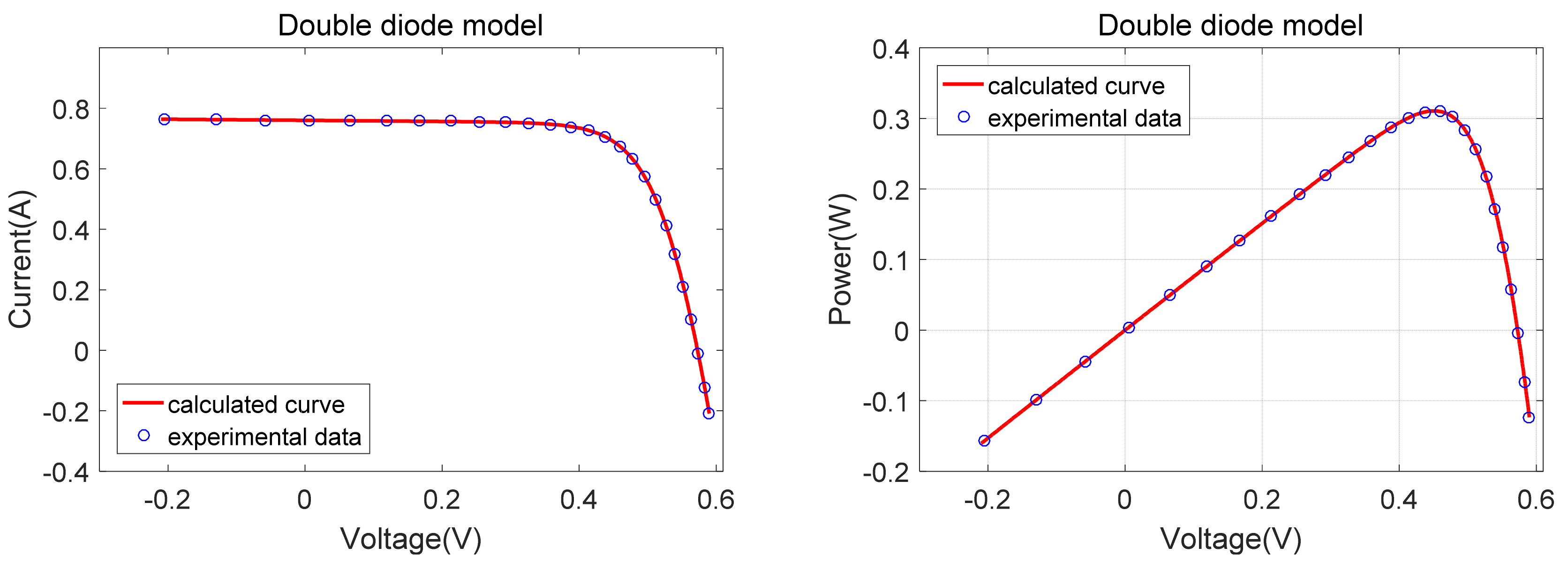
For DDM, the extraction of seven parameters increases the difficulty of parameter identification. Table 7 illustrates the best parameters and RMSE obtained for all selected algorithms. The overall best RMSE value of all compared algorithms are indicated in bold. It is obvious from Table 7 that CSOOJAYA, DE/WOA, EJADE, MTLBO, ITLBO, CPMPSO, DERAO have the smallest RMSE (9.8248 × 10⁻⁴), followed by MLBSA and MPPCEDE. To further verify the accuracy of the results, Figure 6 illustrates the best results obtained using CSOOJAYA to plot the I-V and P-V curves. Obviously, the data calculated by CSOOJAYA are in good agreement with the measured data across the entire voltage range.
The IAE of power and current are shown in Table 8. All values of are less than 2.54 × 10⁻³ and all values of are less than 1.48 × 10⁻³, which demonstrates the accuracy of CSOOJAYA parameter identification.
5.3. Results on the PV Module
The effectiveness of CSOOJAYA is further verified using the PhotoWatt-PWP201 PV module. Table 9 illustrates the best parameters and RMSE obtained for all selected algorithms. The overall best RMSE value of all the compared algorithms are marked in bold. Among all the comparison algorithms, CSOOJAYA, DE/WOA, MLBSA, EJADE, MTLBO, MPPCEDE, MADE, ITLBO, CPMPSO, PGJAYA, IJAYA, LCJAYA and DERAO obtained the best RMSE value, followed by JAYA. To further verify the accuracy of the results, Figure 7 illustrates the best results obtained using CSOOJAYA to plot the I-V and P-V curves. Obviously, the data calculated by CSOOJAYA are in good agreement with the measured data across the entire voltage range. The IAE of power and current are shown in Table 10. All values of are less than 4.83 × 10⁻³ and all values of are less than 7.99 × 10⁻², which verifies the accuracy of CSOOJAYA parameter identification again.
5.4. Statistical Results and Convergence Curve
The above three sections demonstrate the superior accuracy of CSOOJAYA in solving parameter identification on different PV models. However, convergence and robustness should also be considered. Therefore, this section compares the convergence curves and statistical results of the three PV models.
The maximum RMSE (Max), minimum RMSE(Min), average RMSE (Mean) and standard deviation (SD) of RMSE obtained by running all the comparison algorithms 30 times independently on three different PV models are shown in Table 11. The overall best RMSE values for all compared algorithms are marked in bold. where Max represents the worst accuracy, Min is the best accuracy, and Mean is the average accuracy, and SD represents the stability of algorithm. It can be seen from the Table 11:
- (1)
- For the best RMES value, only CSOOJAYA, DE/WOA, EJADE, MTLBO, ITLBO, CPMPSO and DERAO get the best RMSE values for all PV models.
- (2)
- For the worst RMSE value, only CSOOJAYA and DE/WOA can obtain the optimal worst value of all PV models
- (3)
- For the average RMSE value, only CSOOJAYA can obtain the optimal average value for all PV models.
- (4)
- Taking into account the SD, it can reflect the reliability of the algorithm. Although the SD of MTLBO, MPPCEDE, ITLBO, CPMPSO and DERAO are slightly better than those of the CSOOJAYA algorithm in the SDM and the PV module, the SD of CSOOJAYA is far superior to other algorithms in the DDM. On the whole, the CSOOJAYA algorithm has stronger reliability than other algorithms. Based on the superior stability and accuracy of three PV models, CSOOJAYA can obtain the best parameter identification results.
In order to validate the convergence speed of CSOOJAYA, Figure 8, Figure 9 and Figure 10 plot the iterative curves of several algorithms on the PV models. Obviously, CSOOJAYA not only get the best results among these three models, but also converges faster than other algorithms.
In summary, the above comparison shows that CSOOJAYA has faster convergence, better accuracy and robustness in extracting the parameters of PV models. Furthermore, the behavior of CSOOJAYA is competitive when compared to other algorithms.
6. Conclusions
This paper proposes a chaotic second order oscillation JAYA algorithm to provide an accurate and stable way to identify the PV parameters. The algorithm introduces the logical chaotic map strategy, and the generated random sequence numbers are non-periodic and non-convergent, which can enhance the diversity of the population and improve the exploration. In order to improve and balance the above two abilities, the second order oscillation strategy is introduced into the algorithm. The strategy can not only maintain the diversity of the population, but also has strong exploration ability due to the oscillation convergence of the solution vector in the early iteration; The solution vector converges asymptotically in the later iteration and has strong exploitation ability. In order to balance the exploitation and exploration as a whole, the self-adaptive weight mechanism is introduced to adjust the tendency of individuals to approach the optimal solution and escape the worst solution and improve the search efficiency of the population and the exploitation. The introduction of mutation mechanisms ensures that individuals avoid getting stuck in local optima. In order to validate the behavior of CSOOJAYA, which is employed to the parameter identification problem of PV models. Finally, the experimental results present that CSOOJAYA delivers excellent behavior in the aspects of convergence, reliability and accuracy.
The data of the PV cells used in this article are measured under certain temperature and light irradiance conditions. In order to further verify the applicability of CSOOJAYA algorithm to parameter identification under different PV cell or module operating scenarios. The next step of the research group will be to study the parameter identification of PV cells or components in multiple scenarios.
Author Contributions
Conceptualization, X.J.; methodology, X.J.; software, Y.C.; validation, Y.C.; writing—original draft preparation, X.J.; writing—review and editing, Y.C.; supervision, X.J. All authors have read and agreed to the published version of the manuscript.
Funding
This research was funded by the National Natural Science Foundation of China (NSFC), grant number 11774017.
Institutional Review Board Statement
Not applicable.
Informed Consent Statement
Not applicable.
Data Availability Statement
The data that support the findings of this study are available from the corresponding author upon reasonable request.
Conflicts of Interest
The authors declare no conflict of interest.
References
- Liang, J.; Ge, S.; Qu, B. Classified perturbation mutation based particle swarm optimization algorithm for parameters extraction of photovoltaic models. Energy Convers. Manag. 2020, 203, 112138.1–112138.20. [Google Scholar] [CrossRef]
- Li, S.; Gong, W.; Yan, X. Parameter extraction of photovoltaic models using an improved teaching-learning-based optimization. Energy Convers. Manag. 2019, 186, 293–305. [Google Scholar] [CrossRef]
- Liu, Y.; Chong, G.; Heidari, A.A.; Chen, H.; Liang, G.; Ye, X.; Cai, Z.; Wang, M. Horizontal and vertical crossover of Harris hawk optimizer with Nelder-Mead simplex for parameter estimation of photovoltaic models. Energy Convers. Manag. 2020, 223, 113211. [Google Scholar] [CrossRef]
- Abd, M.; Oliva, D. Parameter estimation of solar cells diode models by an improved opposition-based whale optimization algorithm. Energy Convers. Manag. 2018, 171, 1843–1859. [Google Scholar]
- Yu, K.; Liang, J.; Qu, Y. Multiple learning backtracking search algorithm for estimating parameters of photovoltaic models. Appl. Energy 2018, 226, 408–422. [Google Scholar] [CrossRef]
- Abdel, M.; Mohamed, R.; Mirjalili, S. Solar photovoltaic parameter estimation using an improved equilibrium optimizer. Sol. Energy 2020, 209, 694–708. [Google Scholar] [CrossRef]
- Xiong, G.; Zhang, J.; Shi, D. Parameter extraction of solar photovoltaic models using an improved whale optimization algorithm. Energy Convers. Manag. 2018, 174, 388–405. [Google Scholar] [CrossRef]
- Yu, K.; Qu, B.; Yue, C. A performance-guided JAYA algorithm for parameters identification of photovoltaic cell and module. Appl. Energy 2019, 237, 241–257. [Google Scholar] [CrossRef]
- Premkumar, M.; Jangir, P.; Sowmya, R.; Elavarasan, R.M.; Kumar, B.S. Enhanced chaotic JAYA algorithm for parameter estimation of photovoltaic cell/module. ISA Trans. 2021, 116, 139–166. [Google Scholar] [CrossRef]
- Zhang, Y.; Ma, M.; Jin, Z. Comprehensive learning Jaya algorithm for parameter extraction of photovoltaic models. Energy 2020, 211, 118644. [Google Scholar] [CrossRef]
- Xiong, G.; Zhang, J.; Yuan, X. Parameter extraction of solar photovoltaic models by means of a hybrid differential evolution with whale optimization algorithm. Sol. Energy 2018, 176, 742–761. [Google Scholar] [CrossRef]
- Wei, D.; Wei, M.; Cai, H. Parameters extraction method of PV model based on key points of I-V curve. Energy Convers. Manag. 2020, 180, 112656.1–112656.8. [Google Scholar] [CrossRef]
- Ibrahim, H.; Anani, N. Evaluation of Analytical Methods for Parameter Extraction of PV modules. Energy Procedia 2017, 134, 69–78. [Google Scholar] [CrossRef]
- Abdel, M.; El-Shahat, D.; Chakrabortty, K. Parameter estimation of photovoltaic models using an improved marine predators algorithm. Energy Convers. Manag. 2021, 227, 113491. [Google Scholar] [CrossRef]
- Song, Y.; Wu, D.; Deng, W. MPPCEDE: Multi-population parallel co-evolutionary differential evolution for parameter optimization. Energy Convers. Manag. 2021, 228, 113661. [Google Scholar] [CrossRef]
- Abdel-Basset, M.; Mohamed, R.; Chakrabortty, R.K.; Sallam, K.; Ryan, M.J. An efficient teaching-learning-based optimization algorithm for parameters identification of photovoltaic models: Analysis and validations. Energy Convers. Manag. 2021, 227, 113614. [Google Scholar] [CrossRef]
- Pardhu, B.G.; Kota, V.R. Radial movement optimization based parameter extraction of double diode model of solar photovoltaic cell. Sol. Energy 2021, 213, 312–327. [Google Scholar] [CrossRef]
- Nunes, H.G.; Silva, P.N.; Pombo, J.A.; Mariano, S.J.; Calado, M.R. Multiswarm spiral leader particle swarm optimization algorithm for PV parameter identification. Energy Convers. Manag. 2020, 225, 113388. [Google Scholar] [CrossRef]
- Yu, K.; Chen, X.; Wang, X. Parameters identification of photovoltaic models using self-adaptive teaching-learning-based optimization. Energy Convers. Manag. 2017, 145, 233–246. [Google Scholar] [CrossRef]
- Tao, Y.; Bai, J.; Pachauri, K. Parameter extraction of photovoltaic modules using a heuristic iterative algorithm. Energy Convers. Manag. 2020, 224, 113386. [Google Scholar] [CrossRef]
- Gao, X.; Cui, Y.; Hu, J.; Xu, G.; Yu, Y. Lambert W-function based exact representation for double diode model of solar cells: Comparison on fitness and parameter extraction. Energy Convers. Manag. 2016, 127, 443–460. [Google Scholar] [CrossRef]
- Li, S.; Gu, Q.; Gong, W. An enhanced adaptive differential evolution algorithm for parameter extraction of photovoltaic models. Energy Convers. Manag. 2020, 205, 112443. [Google Scholar] [CrossRef]
- Li, S.; Gong, W.; Yan, X. Parameter estimation of photovoltaic models with memetic adaptive differential evolution. Sol. Energy 2019, 190, 465–474. [Google Scholar] [CrossRef]
- Lekouaghet, B.; Boukabou, A.; Chabane, B. Estimation of the photovoltaic cells/Modules parameters using an improved Rao-based chaotic optimization technique. Energy Convers. Manag. 2021, 229, 113722. [Google Scholar] [CrossRef]
- Jian, X.; Zhu, Y. Parameters identification of photovoltaic models using modified Rao-1 optimization algorithm. Optik 2021, 231, 166439. [Google Scholar] [CrossRef]
- Sallam, M.; Hossain, A.; Chakrabortty, K. An Improved Gaining-Sharing Knowledge Algorithm for Parameter Extraction of Photovoltaic Models. Energy Convers. Manag. 2021, 237, 114030. [Google Scholar] [CrossRef]
- Khan, A.; Ahmad, S.; Sarwar, A. Chaos Induced Coyote Algorithm (CICA) for Extracting the Parameters in a Single, Double, and Three Diode Model of a Mono-Crystalline, Polycrystalline, and a Thin-Film Solar PV Cell. Electronics 2021, 10, 2094. [Google Scholar] [CrossRef]
- Yu, K.; Liang, J.; Qu, Y. Parameters identification of photovoltaic models using an improved JAYA optimization algorithm. Energy Convers. Manag. 2017, 150, 742–753. [Google Scholar] [CrossRef]
- Jian, X.; Weng, Z. A logistic chaotic JAYA algorithm for parameters identification of photovoltaic cell and module models. Optik 2019, 203, 164041. [Google Scholar] [CrossRef]
- Wang, L.; Huang, C. A novel Elite Opposition-based Jaya algorithm for parameter estimation of photovoltaic cell models. Optik 2020, 203, 164034. [Google Scholar] [CrossRef]
- Venkata, R. Jaya: A simple and new optimization algorithm for solving constrained and unconstrained optimization problems. Int. J. Ind. Eng. Comput. 2016, 7, 19–34. [Google Scholar] [CrossRef]
Figure 1.
The equivalent circuit of SDM.

Figure 2.
The equivalent circuit of DDM.

Figure 3.
The equivalent circuit of a PV module.

Figure 4.
The flowchart of CSOOJAYA.

Figure 5.
Experimental and calculated data of CSOOJAYA for SDM.

Figure 6.
Experimental and calculated data of CSOOJAYA for DDM.

Figure 7.
Experimental and calculated data of CSOOJAYA for PV module.

Figure 8.
Convergence curves of the seven algorithms on SDM.

Figure 9.
Convergence curves of the seven algorithms on DDM.

Figure 10.
Convergence curves of the seven algorithms on PV.


Table 1.
The characteristics of the three methods.
| Method | Characteristic | Instance |
|---|---|---|
| Analytical method |
| |
| Deterministic method |
| Newton–Raphson method [16,17], iterative curve fitting [18,19] and Lambert W-function [20,21] |
| Heuristic method |
| CPMPSO [1], MTLBO [16], MSLPSO [18], EJADE [22], MADE [23], MRAO-1 [25] |
Table 2.
Summary of some existing heuristic methods.
| Algorithm | Summary |
|---|---|
| CPMPSO [1] |
|
| PGJAYA [8] |
|
| CLJAYA [10] |
|
| MTLBO [16] | According to the score level of each learner, each teaching stage is divided into three levels to update the population. |
| MSLPSO [18] |
|
| EJADE [22] |
|
| MADE [23] |
|
| MRAO-1 [25] |
|
| IGSK [26] |
|
| CICA [27] |
|
| IJAYA [28] |
|
| LCJAYA [29] |
|
| EO-JAYA [30] |
|
Table 3.
Parameters ranges of PV models.
| Parameter | SDM/DDM | PV Module | ||
|---|---|---|---|---|
| Lower | Upper | Lower | Upper | |
| 0 | 1 | 0 | 2 | |
| 0 | 1 | 0 | 50 | |
| 0 | 0.5 | 0 | 2 | |
| 0 | 100 | 0 | 2000 | |
| 1 | 2 | 1 | 50 | |
Table 4.
Parameter settings of the compared algorithms.
| Algorithm | Parameters |
|---|---|
| DE/WOA | Np = 40, F = rand (0.1,1), Cr = rand (0,1) |
| MLBSA | Np = 50 |
| EJADE | = 50, = 4 |
| MTLBO | Np = 50 |
| MPPCEDE | Np = 40; F = rand (0.1,1); Cr = rand (0,1) |
| MADE | NP = 20; 0.05 for the SDM and PV module; 0.01 for the DDM |
| IJAYA | NP = 20 |
| ITLBO | Np = 50 |
| CPMPSO | NP = 50, w = 0.729, c1 = 1.49455, c2 = 1.49455 |
| DERAO | NP = 20 |
| JAYA | NP = 20 |
| PGJAYA | NP = 20 |
| LCJAYA | NP = 20 |
| CSOOJAYA | NP = 20 |
Table 5.
Comparison of the extracted optimal parameters of the SDM.
| Algorithm | (A) | (A) | () | () | n | RMSE |
|---|---|---|---|---|---|---|
| DE/WOA | 0.760776 | 0.323021 | 0.036377 | 53.718524 | 1.481184 | 9.860219 × 10⁻⁴ |
| MLBSA | 0.7608 | 0.32302 | 0.0364 | 53.7185 | 1.4812 | 9.8602 × 10⁻⁴ |
| EJADE | 0.7608 | 0.3230 | 0.0364 | 53.7185 | 1.4812 | 9 8602 × 10−4 |
| MTLBO | 0.76077553 | 0.32300 | 0.03637709 | 53.7185251 | 1.48118359 | 9 860219 × 10−4 |
| MPPCEDE | 0.7608 | 0.32302 | 0.0364 | 53.7185 | 1.4812 | 9.8602 × 10⁻⁴ |
| MADE | 0.7608 | 0.3230 | 0.0364 | 53.7185 | 1.4812 | 9.8602 × 10⁻⁴ |
| IJAYA | 0.7608 | 0.3228 | 0.0364 | 53.7595 | 1.4811 | 9.8603 × 10⁻⁴ |
| ITLBO | 0.7608 | 0.3230 | 0.0364 | 53.7185 | 1.4812 | 9.8602 × 10⁻⁴ |
| CPMPSO | 0.760776 | 0.323021 | 0.036377 | 53.718522 | 1.481184 | 9.860219 × 10⁻⁴ |
| DERAO | 0.760776 | 0.323021 | 0.036377 | 53.718522 | 1.481135 | 9.860219 × 10⁻⁴ |
| JAYA | 0.7608 | 0.3281 | 0.0364 | 54.9298 | 1.4828 | 9.8946 × 10⁻⁴ |
| PGJAYA | 0.7608 | 0.3230 | 0.0364 | 53.7185 | 1.4812 | 9.8602 × 10⁻⁴ |
| LCJAYA | 0.7608 | 0.3230 | 0.0364 | 53.7185 | 1.4819 | 9.8602 × 10⁻⁴ |
| CSOOJAYA | 0.760776 | 0.323021 | 0.036377 | 53.718525 | 1.481184 | 9.860219 × 10⁻⁴ |
Table 6.
IAE of CSOOJAYA for the SDM.
| Item | ||||||
|---|---|---|---|---|---|---|
| 1 | −0.2057 | 0.7640 | 0.7640881747 | 0.0000881747 | −0.1571729375 | 0.0000181375 |
| 2 | −0.1291 | 0.7620 | 0.7626635570 | 0.0006635570 | −0.0984598652 | 0.0000856652 |
| 3 | −0.0588 | 0.7605 | 0.7613557780 | 0.0008557780 | −0.0447677197 | 0.0000503197 |
| 4 | 0.0057 | 0.7605 | 0.7601544618 | 0.0003455381 | 0.0043328804 | 0.0000019695 |
| 5 | 0.0646 | 0.7600 | 0.7590556797 | 0.0009443202 | 0.0490349969 | 0.0000610030 |
| 6 | 0.1185 | 0.7590 | 0.7580428161 | 0.0009571838 | 0.0898280737 | 0.0001134262 |
| 7 | 0.1678 | 0.7570 | 0.7570921248 | 0.0000921248 | 0.1270400585 | 0.0000154585 |
| 8 | 0.2132 | 0.7570 | 0.7561418358 | 0.0008581641 | 0.1612094393 | 0.0001829606 |
| 9 | 0.2545 | 0.7555 | 0.7550873439 | 0.0004126560 | 0.1921697290 | 0.0001050209 |
| 10 | 0.2924 | 0.7540 | 0.7536643499 | 0.0003356500 | 0.2203714559 | 0.0000981440 |
| 11 | 0.3269 | 0.7505 | 0.7513914392 | 0.0008914392 | 0.2456298615 | 0.0002914115 |
| 12 | 0.3585 | 0.7465 | 0.7473543260 | 0.0008543260 | 0.2679265258 | 0.0003062758 |
| 13 | 0.3873 | 0.7385 | 0.7401176997 | 0.0016176997 | 0.2866475851 | 0.0006265351 |
| 14 | 0.4137 | 0.7280 | 0.7273827075 | 0.0006172924 | 0.3009182261 | 0.0002553738 |
| 15 | 0.4373 | 0.7065 | 0.7069731390 | 0.0004731390 | 0.3091593537 | 0.0002069037 |
| 16 | 0.4590 | 0.6755 | 0.6752806425 | 0.0002193574 | 0.3099538149 | 0.0001006850 |
| 17 | 0.4784 | 0.6320 | 0.6307587591 | 0.0012412408 | 0.3017549903 | 0.0005938096 |
| 18 | 0.4960 | 0.5730 | 0.5719288231 | 0.0010711768 | 0.2836766963 | 0.0005313036 |
| 19 | 0.5119 | 0.4990 | 0.4996074317 | 0.0006074317 | 0.2557490442 | 0.0003109442 |
| 20 | 0.5265 | 0.4130 | 0.4136491106 | 0.0006491106 | 0.2177862567 | 0.0003417567 |
| 21 | 0.5398 | 0.3165 | 0.3175102788 | 0.0010102788 | 0.1713920485 | 0.0005453485 |
| 22 | 0.5521 | 0.2120 | 0.2121548945 | 0.0001548945 | 0.1171307172 | 0.0000855172 |
| 23 | 0.5633 | 0.1035 | 0.1022509879 | 0.0012490120 | 0.0575979815 | 0.0007035684 |
| 24 | 0.5736 | −0.0100 | −0.0087182129 | 0.0012817870 | −0.0050007669 | 0.0007352330 |
| 25 | 0.5833 | −0.1230 | −0.1255085017 | 0.0025085017 | −0.0732091090 | 0.0014632090 |
| 26 | 0.5900 | −0.2100 | −0.2084737660 | 0.0015262339 | −0.1229995219 | 0.0009004780 |
Table 7.
Comparison of the extracted optimal parameters of the DDM.
| Algorithm | (A) | (A) | (A) | () | () | n1 | n2 | RMSE |
|---|---|---|---|---|---|---|---|---|
| DE/WOA | 0.760781 | 0.225974 | 0.749346 | 0.036740 | 55.485437 | 1.451017 | 2 | 9.824849 × 10⁻⁴ |
| MLBSA | 0.7608 | 0.22728 | 0.73835 | 0.0367 | 55.4612 | 1.4515 | 2 | 9.8249 × 10⁻⁴ |
| EJADE | 0.7608 | 0.2260 | 0.7493 | 0.0367 | 55.4854 | 1.4510 | 2 | 9.8248 × 10⁻⁴ |
| MTLBO | 0.7607810 | 0.22597 | 0.7493 | 0.03674043 | 55.485447 | 1.451016 | 2 | 9.824849 × 10⁻⁴ |
| MPPCEDE | 0.7608 | 0.22728 | 0.73835 | 0.0367 | 55.4612 | 1.4515 | 2 | 9.82485 × 10⁻⁴ |
| MADE | 0.7608 | 0.2246 | 0.7394 | 0.0368 | 55.4329 | 1.4505 | 1.9963 | 9.8261 × 10⁻⁴ |
| IJAYA | 0.7601 | 0.0050445 | 0.75094 | 0.0376 | 77.8519 | 1.2186 | 1.6247 | 9.8293 × 10⁻⁴ |
| ITLBO | 0.7608 | 0.2260 | 0.7493 | 0.0367 | 55.4854 | 1.4510 | 2 | 9.8248 × 10⁻⁴ |
| CPMPSO | 0.76078 | 0.22597 | 0.74935 | 0.03674 | 55.48544 | 1.45102 | 2 | 9.824849 × 10⁻⁴ |
| DERAO | 0.760781 | 0.225959 | 0.749667 | 0.036740 | 55.486045 | 1.450963 | 2 | 9.824849 × 10⁻⁴ |
| JAYA | 0.7607 | 0.0060763 | 0.31507 | 0.0364 | 52.6575 | 1.4788 | 1.8436 | 9.8934 × 10⁻⁴ |
| PGJAYA | 0.7608 | 0.21031 | 0.88534 | 0.0368 | 55.8135 | 1.4450 | 2 | 9.8263 × 10⁻⁴ |
| LCJAYA | 0.7608 | 0.22596 | 0.74640 | 0.0367 | 55.4815 | 1.4518 | 2.0000 | 9.8250 × 10⁻⁴ |
| CSOOJAYA | 0.760781 | 0.225974 | 0.749345 | 0.036740 | 55.485437 | 1.451017 | 2.000000 | 9.824849 × 10⁻⁴ |
Table 8.
IAE of CSOOJAYA for the DDM.
| Item | ||||||
|---|---|---|---|---|---|---|
| 1 | −0.2057 | 0.7640 | 0.7639834118 | 0.0000165881 | −0.1571513878 | 0.0000034121 |
| 2 | −0.1291 | 0.7620 | 0.7626040957 | 0.0006040957 | −0.0984521887 | 0.0000779887 |
| 3 | −0.0588 | 0.7605 | 0.7613376980 | 0.0008376980 | −0.0447666566 | 0.0000492566 |
| 4 | 0.0057 | 0.7605 | 0.7601737877 | 0.0003262122 | 0.0043329905 | 0.0000018594 |
| 5 | 0.0646 | 0.7600 | 0.7591076801 | 0.0008923198 | 0.0490383561 | 0.0000576438 |
| 6 | 0.1185 | 0.7590 | 0.7581214198 | 0.0008785801 | 0.0898373882 | 0.0001041117 |
| 7 | 0.1678 | 0.7570 | 0.7571886136 | 0.0001886136 | 0.1270562493 | 0.0000316493 |
| 8 | 0.2132 | 0.7570 | 0.7562436068 | 0.0007563931 | 0.1612311369 | 0.0001612630 |
| 9 | 0.2545 | 0.7555 | 0.7551773015 | 0.0003226984 | 0.1921926232 | 0.0000821267 |
| 10 | 0.2924 | 0.7540 | 0.7537223535 | 0.0002776464 | 0.2203884161 | 0.0000811838 |
| 11 | 0.3269 | 0.7505 | 0.7513991342 | 0.0008991342 | 0.2456323769 | 0.0002939269 |
| 12 | 0.3585 | 0.7465 | 0.7473014432 | 0.0008014432 | 0.2679075674 | 0.0002873174 |
| 13 | 0.3873 | 0.7385 | 0.7400106607 | 0.0015106607 | 0.2866061288 | 0.0005850788 |
| 14 | 0.4137 | 0.7280 | 0.7272469525 | 0.0007530474 | 0.3008620642 | 0.0003115357 |
| 15 | 0.4373 | 0.7065 | 0.7068502977 | 0.0003502977 | 0.3091056352 | 0.0001531852 |
| 16 | 0.4590 | 0.6755 | 0.6752105425 | 0.0002894574 | 0.3099216390 | 0.0001328609 |
| 17 | 0.4784 | 0.6320 | 0.6307607576 | 0.0012392423 | 0.3017559464 | 0.0005928535 |
| 18 | 0.4960 | 0.5730 | 0.5719947329 | 0.0010052670 | 0.2837093875 | 0.0004986124 |
| 19 | 0.5119 | 0.4990 | 0.4997061352 | 0.0007061352 | 0.2557995706 | 0.0003614706 |
| 20 | 0.5265 | 0.4130 | 0.4137336728 | 0.0007336728 | 0.2178307787 | 0.0003862787 |
| 21 | 0.5398 | 0.3165 | 0.3175462057 | 0.0010462057 | 0.1714114418 | 0.0005647418 |
| 22 | 0.5521 | 0.2120 | 0.2121229960 | 0.0001229960 | 0.1171131061 | 0.0000679061 |
| 23 | 0.5633 | 0.1035 | 0.1021632765 | 0.0013367234 | 0.0575485736 | 0.0007529763 |
| 24 | 0.5736 | −0.0100 | −0.0087917509 | 0.0012082490 | −0.0050429483 | 0.0006930516 |
| 25 | 0.5833 | −0.1230 | −0.1255434350 | 0.0025434350 | −0.0732294856 | 0.0014835856 |
| 26 | 0.5900 | −0.2100 | −0.2083715891 | 0.0016284108 | −0.1229392376 | 0.0009607623 |
Table 9.
Comparison of the extracted optimal parameters of the PV module.
| Algorithm | (A) | (A) | () | () | n | RMSE |
|---|---|---|---|---|---|---|
| DE/WOA | 1.030514 | 3.482263 | 1.201271 | 981.982143 | 48.642835 | 2.425075 × 10⁻³ |
| MLBSA | 1.0305 | 3.4823 | 1.2013 | 981.9823 | 48.6428 | 2.4251 × 10⁻³ |
| EJADE | 1.0305 | 3.4823 | 1.2013 | 981.9824 | 48.6428 | 2.4251 × 10⁻³ |
| MTLBO | 1.0305143 | 3.4823 | 1.2012710 | 981.9823732 | 48.6428349 | 2425075 × 10−3 |
| MPPCEDE | 1.030514 | 3.482263 | 1.201271 | 981.982143 | 48.642835 | 2.42507 × 10⁻³ |
| MADE | 1.0305 | 3.4823 | 1.2013 | 981.9823 | 48.6428 | 2.4250 × 10⁻³ |
| IJAYA | 1.0305 | 3.4703 | 1.2016 | 977.3752 | 48.6298 | 2.4251 × 10⁻³ |
| ITLBO | 1.0305 | 3.4823 | 1.2013 | 981.9823 | 48.6428 | 2.4251 × 10⁻³ |
| CPMPSO | 1.030514 | 3.4823 | 1.201271 | 981.9823 | 48.64284 | 2.425075 × 10⁻³ |
| DERAO | 1.030514 | 3.4823 | 1.201271 | 981.9821 | 48.64131 | 2.425075 × 10⁻³ |
| JAYA | 1.0302 | 3.4931 | 1.2014 | 1022.5 | 48.6531 | 2.427785 × 10⁻³ |
| PGJAYA | 1.0305 | 3.4818 | 1.2013 | 981.8545 | 48.6424 | 2.425075 × 10⁻³ |
| LCJAYA | 1.0305 | 3.4823 | 1.2024 | 981.9828 | 48.6684 | 2.425075 × 10⁻³ |
| CSOOJAYA | 1.030514 | 3.482263 | 1.201271 | 981.982243 | 48.642834 | 2.425075 × 10⁻³ |
Table 10.
IAE of CSOOJAYA for PV module.
| Item | ||||||
|---|---|---|---|---|---|---|
| 1 | 0.1248 | 1.0315 | 1.0291188622 | 0.0023811377 | 0.1284340340 | 0.0002971659 |
| 2 | 1.8093 | 1.0300 | 1.0273807740 | 0.0026192259 | 1.8588400345 | 0.0047389654 |
| 3 | 3.3511 | 1.0260 | 1.0257414978 | 0.0002585021 | 3.4373623333 | 0.0008662666 |
| 4 | 4.7622 | 1.0220 | 1.0241068556 | 0.0021068556 | 4.8770016680 | 0.0100332680 |
| 5 | 6.0538 | 1.0180 | 1.0222915054 | 0.0042915054 | 6.1887483154 | 0.0259799154 |
| 6 | 7.2364 | 1.0155 | 1.0199303816 | 0.0044303816 | 7.3806242138 | 0.0320600138 |
| 7 | 8.3189 | 1.0140 | 1.0163628063 | 0.0023628063 | 8.4550205496 | 0.0196559496 |
| 8 | 9.3097 | 1.0100 | 1.0104958517 | 0.0004958517 | 9.4074132312 | 0.0046162312 |
| 9 | 10.2163 | 1.0035 | 1.0006286698 | 0.0028713301 | 10.2227226794 | 0.0293343705 |
| 10 | 11.0449 | 0.9880 | 0.9845480779 | 0.0034519220 | 10.8742350664 | 0.0381261335 |
| 11 | 11.8018 | 0.9630 | 0.9595213746 | 0.0034786253 | 11.3240793592 | 0.0410540407 |
| 12 | 12.4929 | 0.9255 | 0.9228385152 | 0.0026614847 | 11.5289292866 | 0.0332496633 |
| 13 | 13.1231 | 0.8725 | 0.8725993581 | 0.0000993581 | 11.4512086365 | 0.0013038865 |
| 14 | 13.6983 | 0.8075 | 0.8072739566 | 0.0002260433 | 11.0582808396 | 0.0030964103 |
| 15 | 14.2221 | 0.7265 | 0.7283361680 | 0.0018361680 | 10.3584698161 | 0.0261141661 |
| 16 | 14.6995 | 0.6345 | 0.6371376868 | 0.0026376868 | 9.3656054279 | 0.0387726779 |
| 17 | 15.1346 | 0.5345 | 0.5362127464 | 0.0017127464 | 8.1153654320 | 0.0259217320 |
| 18 | 15.5311 | 0.4275 | 0.4295110044 | 0.0020110044 | 6.6707783610 | 0.0312331110 |
| 19 | 15.8929 | 0.3185 | 0.3187741584 | 0.0002741584 | 5.0662458227 | 0.0043571727 |
| 20 | 16.2229 | 0.2085 | 0.2073891784 | 0.0011108215 | 3.3644539035 | 0.0180207464 |
| 21 | 16.5241 | 0.1010 | 0.0961668397 | 0.0048331602 | 1.5890704768 | 0.0798636231 |
| 22 | 16.7987 | −0.0080 | −0.0083257217 | 0.0003257217 | −0.1398613011 | 0.0054717011 |
| 23 | 17.0499 | −0.1110 | −0.1109368217 | 0.0000631782 | −1.8914617173 | 0.0010771826 |
| 24 | 17.2793 | −0.2090 | −0.2092476082 | 0.0002476082 | −3.6156521970 | 0.0042784970 |
| 25 | 17.4885 | −0.3030 | −0.3008639322 | 0.0021360677 | −5.2616588799 | 0.0373566200 |
Table 11.
Comparison of statistical results for PV models.
| Model | Algorithm | RMSE | |||
|---|---|---|---|---|---|
| Min | Max | Mean | SD | ||
| SDM | DE/WOA | 9.860219 × 10⁻⁴ | 9.860219 × 10⁻⁴ | 9.860219 × 10⁻⁴ | 3.545178 × 10⁻¹⁷ |
| MLBSA | 9.8602 × 10⁻⁴ | 9.8602 × 10⁻⁴ | 9.8602 × 10⁻⁴ | 9.1461 × 10⁻¹² | |
| EJADE | 9.8602 × 10⁻⁴ | 9.8602 × 10⁻⁴ | 9.8602 × 10⁻⁴ | 5.13 × 10⁻¹⁷ | |
| MTLBO | 9.860219 × 10⁻⁴ | 9.860219 × 10⁻⁴ | 9.860219 × 10⁻⁴ | 1.9092749 × 10⁻¹⁷ | |
| MPPCEDE | 9.86022 × 10⁻⁴ | 9.86022 × 10⁻⁴ | 9.86022 × 10⁻⁴ | 2.44932 × 10⁻¹⁷ | |
| MADE | 9.8602 × 10⁻⁴ | 9.8602 × 10⁻⁴ | 9.8602 × 10⁻⁴ | 2.74 × 10⁻¹⁵ | |
| IJAYA | 9.8603 × 10⁻⁴ | 1.0622 × 10⁻³ | 9.9204 × 10⁻⁴ | 1.4033 × 10⁻⁵ | |
| ITLBO | 9.8602 × 10⁻⁴ | 9.8602 × 10⁻⁴ | 9.8602 × 10⁻⁴ | 2.19 × 10⁻¹⁷ | |
| CPMPSO | 9.86022 × 10⁻⁴ | 9.86022 × 10⁻⁴ | 9.86022 × 10⁻⁴ | 2.17556 × 10⁻¹⁷ | |
| DERAO | 9.860219 × 10⁻⁴ | 9.860219 × 10⁻⁴ | 9.860219 × 10⁻⁴ | 3.642031 × 10⁻¹⁷ | |
| JAYA | 9.8946 × 10⁻⁴ | 1.4783 × 10⁻³ | 1.1617 × 10⁻³ | 1.8796 × 10⁻⁴ | |
| PGJAYA | 9.8602 × 10⁻⁴ | 9.8603 × 10⁻⁴ | 9.8602 × 10⁻⁴ | 1.4485 × 10⁻⁹ | |
| LCJAYA | 9.8602 × 10⁻⁴ | 9.8602 × 10⁻⁴ | 9.8602 × 10⁻⁴ | 5.6997 × 10⁻¹⁶ | |
| CSOOJAYA | 9.860219 × 10⁻⁴ | 9.860219 × 10⁻⁴ | 9.860219 × 10⁻⁴ | 4.717305 × 10⁻¹⁷ | |
| DDM | DE/WOA | 9.824849 × 10⁻⁴ | 9.860377 × 10⁻⁴ | 9.829703 × 10⁻⁴ | 9.152178 × 10⁻⁷ |
| MLBSA | 9.8249 × 10⁻⁴ | 9.8518 × 10⁻⁴ | 9.8798 × 10⁻⁴ | 1.3482 × 10⁻⁶ | |
| EJADE | 9.8248 × 10⁻⁴ | 9.8602 × 10⁻⁴ | 9.8363 × 10⁻⁴ | 1.36 × 10⁻⁶ | |
| MTLBO | 9.824849 × 10⁻⁴ | 9.825026 × 10⁻⁴ | 9.824855 × 10⁻⁴ | 3.30000 × 10⁻⁹ | |
| MPPCEDE | 9.82485 × 10⁻⁴ | 9.82908 × 10⁻⁴ | 9.82504 × 10⁻⁴ | 8.02951 × 10⁻⁸ | |
| MADE | 9.8261 × 10⁻⁴ | 9.8786 × 10⁻⁴ | 9.8608 × 10⁻⁴ | 8.02 × 10⁻⁵ | |
| IJAYA | 9.8293 × 10⁻⁴ | 1.4055 × 10⁻³ | 1.0269 × 10⁻³ | 9.8325 × 10⁻⁵ | |
| ITLBO | 9.8248 × 10⁻⁴ | 9.8812 × 10⁻⁴ | 9.8497 × 10⁻⁴ | 1.54 × 10⁻⁶ | |
| CPMPSO | 9.82485 × 10⁻⁴ | 9.83137 × 10⁻⁴ | 9.86022 × 10⁻⁴ | 1.3398 × 10⁻⁶ | |
| DERAO | 9.824841 × 10⁻⁴ | 9.824897 × 10⁻⁴ | 9.824845 × 10⁻⁴ | 1.01560 × 10⁻⁹ | |
| JAYA | 9.8934 × 10⁻⁴ | 1.4793 × 10⁻³ | 1.1767 × 10⁻³ | 1.9356 × 10⁻⁴ | |
| PGJAYA | 9.8263 × 10⁻⁴ | 9.9499 × 10⁻⁴ | 9.8582 × 10⁻⁴ | 2.5375 × 10⁻⁶ | |
| LCJAYA | 9.8250 × 10⁻⁴ | 9.8602 × 10⁻⁴ | 9.8308 × 10⁻⁴ | 1.3118 × 10⁻⁶ | |
| CSOOJAYA | 9.824849 × 10⁻⁴ | 9.824849 × 10⁻⁴ | 9.824849 × 10⁻⁴ | 5.576332 × 10⁻¹⁷ | |
| PV module | DE/WOA | 2.425075 × 10⁻³ | 2.425442 × 10⁻³ | 2.425092 × 10⁻³ | 6.270718 × 10⁻⁸ |
| MLBSA | 2.425075 × 10⁻³ | 2.425084 × 10⁻³ | 2.425312 × 10⁻³ | 4.336794 × 10⁻⁸ | |
| EJADE | 2.4251 × 10⁻³ | 2.4251 × 10⁻³ | 2.4251 × 10⁻³ | 3.27 × 10⁻¹⁷ | |
| MTLBO | 2.425075 × 10⁻³ | 2.425075 × 10⁻³ | 2.425075 × 10⁻³ | 1.3070107 × 10⁻¹⁷ | |
| MPPCEDE | 2.42507 × 10⁻³ | 2.42507 × 10⁻³ | 2.42507 × 10⁻³ | 2.23156 × 10⁻¹⁷ | |
| MADE | 2.4250 × 10⁻³ | 2.4251 × 10⁻³ | 2.4251 × 10⁻³ | 3.07 × 10⁻¹⁷ | |
| IJAYA | 2.4251 × 10⁻³ | 2.4393 × 10⁻³ | 2.4289 × 10⁻³ | 3.7755 × 10⁻⁶ | |
| ITLBO | 2.4251 × 10⁻³ | 2.4251 × 10⁻³ | 2.4251 × 10⁻³ | 1.27 × 10⁻¹⁷ | |
| CPMPSO | 2.425075 × 10⁻³ | 2.425075 × 10⁻³ | 2.425075 × 10⁻³ | 1.515959 × 10⁻¹⁷ | |
| DERAO | 2.425075 × 10⁻³ | 2.425075 × 10⁻³ | 2.425075 × 10⁻³ | 1.716113 × 10⁻¹⁷ | |
| JAYA | 2.427785 × 10⁻³ | 2.595873 × 10⁻³ | 2.453710 × 10⁻³ | 3.456290 × 10⁻⁵ | |
| PGJAYA | 2.425075 × 10⁻³ | 2.426764 × 10⁻³ | 2.425144 × 10⁻³ | 3.071420 × 10⁻⁷ | |
| LCJAYA | 2.425075 × 10⁻³ | 2.425075 × 10⁻³ | 2.425075 × 10⁻³ | 2.415229 × 10⁻¹⁶ | |
| CSOOJAYA | 2.425075 × 10⁻³ | 2.425075 × 10⁻³ | 2.425075 × 10⁻³ | 2.699858 × 10⁻¹⁷ |
Publisher’s Note: MDPI stays neutral with regard to jurisdictional claims in published maps and institutional affiliations. |
© 2022 by the authors. Licensee MDPI, Basel, Switzerland. This article is an open access article distributed under the terms and conditions of the Creative Commons Attribution (CC BY) license (https://creativecommons.org/licenses/by/4.0/).
Share and Cite
MDPI and ACS Style
Jian, X.; Cao, Y. A Chaotic Second Order Oscillation JAYA Algorithm for Parameter Extraction of Photovoltaic Models. Photonics 2022, 9, 131. https://doi.org/10.3390/photonics9030131
AMA Style
Jian X, Cao Y. A Chaotic Second Order Oscillation JAYA Algorithm for Parameter Extraction of Photovoltaic Models. Photonics. 2022; 9(3):131. https://doi.org/10.3390/photonics9030131
Chicago/Turabian StyleJian, Xianzhong, and Yougang Cao. 2022. "A Chaotic Second Order Oscillation JAYA Algorithm for Parameter Extraction of Photovoltaic Models" Photonics 9, no. 3: 131. https://doi.org/10.3390/photonics9030131
Note that from the first issue of 2016, this journal uses article numbers instead of page numbers. See further details here.