Causality and Renormalization in Finite-Time-Path Out-of-Equilibrium ϕ³ QFT

Abstract

Our aim is to contribute to quantum field theory (QFT) formalisms useful for descriptions of short time phenomena, dominant especially in heavy ion collisions. We formulate out-of-equilibrium QFT within the finite-time-path formalism (FTP) and renormalization theory (RT). The potential conflict of FTP and RT is investigated in $g{\varphi }^3$ QFT, by using the retarded/advanced ($R/A$) basis of Green functions and dimensional renormalization (DR). For example, vertices immediately after (in time) divergent self-energy loops do not conserve energy, as integrals diverge. We “repair” them, while keeping $d<4$, to obtain energy conservation at those vertices. Already in the S-matrix theory, the renormalized, finite part of Feynman self-energy ${\Sigma }_F(p_0)$ does not vanish when $|p_0|\to \infty$ and cannot be split to retarded and advanced parts. In the Glaser–Epstein approach, the causality is repaired in the composite object $G_F(p_0){\Sigma }_F(p_0)$. In the FTP approach, after repairing the vertices, the corresponding composite objects are $G_R(p_0){\Sigma }_R(p_0)$ and ${\Sigma }_A(p_0)G_A(p_0)$. In the limit $d\to 4$, one obtains causal QFT. The tadpole contribution splits into diverging and finite parts. The diverging, constant component is eliminated by the renormalization condition $⟨0\left|\varphi \right|0⟩=0$ of the S-matrix theory. The finite, oscillating energy-nonconserving tadpole contributions vanish in the limit $t\to \infty$.

1. Introduction and Survey

In many regions of physics, the interacting processes are embedded in a medium and require a short-time description. To respond to such demands, neither vacuum S-matrix field theory [1,2,3,4,5], nor equilibrium QFT [6,7,8,9,10,11,12,13,14,15,16] with the Keldysh-time-path [17,18,19,20,21,22,23,24,25,26,27,28] suffice. The features, a short time after the beginning of evolution, where uncertainty relations do not keep energy conserved, are to be treated with the finite-time-path method. Such an approach includes many specific features that are not yet completely understood. A particular problem, almost untreated, is handling of UV divergences of the QFT as seen at finite time. The present paper is devoted to this problem. We consider it in the simplest form of $\lambda {\varphi }^3$ QFT, but many of the discussed features will find their analogs in more advanced QED and QCD.

Starting with perturbation expansion in the coordinate space, one performs the Wigner transform and uses the Wick theorem. The propagators, originally appearing in matrix representation, are linearly connected to the Keldysh base with R, A, and K components. For a finite-time-path, the lowest order propagators and one-loop self-energies taken at $t=\infty$ correspond to Keldysh-time-path propagators and one-loop self-energies. For simplicity, the label “∞” is systematically omitted throughout the paper, except in the Appendix with technical details.

To analyze the vertices, one further separates K-component [27,28] into its retarded (K,R) and advanced (K,A) parts:

$$G_R(p)=G_A(-p)=\frac{-i}{p^2-m^2+2i{p}_0ϵ},$$

$$G_K(p)=2\pi \delta (p^2-m^2)[1+2f({\omega }_p)]$$

$$=G_{K,R}(p)-G_{K,A}(p),$$

$$G_{K,R}(p)=-G_{K,A}(-p)=h(p_0,{\omega }_p)G_R(p),$$

$${\omega }_p=\sqrt{{\overrightarrow{p}}^2+m^2},h(p_0,{\omega }_p)=-\frac{p_0}{{\omega }_p}[1+2f({\omega }_p)].$$

(1)

Matrix propagators are (i and j take the values $1,2$):

$$G_{ij}(p)=\frac{1}{2}[G_K(p)+{(-1)}^j{G}_R(p)+{(-1)}^i{G}_A(p)].$$

(2)

Specifically:

$$G_F(p)=G_{11}{(p)}_{f({\omega }_p)=0}=\frac{-i}{p^2-m^2+2iϵ},G_{\overline{F}}(p)=-G_F^{*}(p).$$

(3)

2. Results

2.1. Conservation and Non-Conservation of Energy at Vertices

Having done all this, one obtains the vertex function (for simplicity, all the four-momenta are arranged to be incoming to the vertex). For the simplicity of discussion, all the times corresponding to the external vertices (j) of the whole diagram are assumed equal ($x_{0,j,ext}=t$, all j; otherwise, some factors, oscillating with time, but inessential for our discussion, would appear), so that the vertex function becomes:

$$\frac{i}{2\pi }\frac{e^{-it{\sum }_i{p}_{0i}}}{{\sum }_i{p}_{0i}+iϵ}.$$

(4)

This expression [27,28,29] integrated over some $d{p}_{o,k}$ by closing the time-path from below gives the expected energy conserving $\delta ({\sum }_i{p}_{0i})$, with the oscillating factor reduced to one. If the integration path catches additional singularity, say the propagator’s $D(p_k)$ pole at ${\overline{p}}_{0k}$, for this contribution, conservation of energy is “spoiled” by a finite amount $\Delta E={\sum }_i^{\prime }{p}_{0i}+{\overline{p}}_{0k}$, and there is an oscillating vertex function $(i/2\pi )e^{-it\Delta E}/(\Delta E+iϵ)$. Note: the fact that some time is lower or higher than another, i.e., $t_1>t_2$ or $t_1<t_2$, survives Wigner transform in the character of ordering (retarded or advanced) of the two-point function.

In general, we have the following possibilities:

• If the vertex time is lower than the other times of all incoming propagators, there are additional contributions, and energy is not conserved at this vertex. The oscillations are just what we would expect from the Heisenberg uncertainty relations. It is how the time dependence emerges in the finite-time-path out-of-equilibrium QFT. The ill-defined pinching singularities—products of retarded and advanced propagators with the same $(p_0,\overrightarrow{p})$, only partially eliminated for the Keldysh time-path [30]—do not appear here as the propagator energies $p_0$ and $p_0^{\prime }$ are different variables, so that the singularities do not coincide except at the point $p_0=p_0^{\prime }$. Thus, the pertinent mathematical expressions are well defined.
• For some vertices, at least one incoming propagator $G(p_{0k})$ is advanced (or more generally, time is lower at the other vertex of this propagator); then, integration over the $p_{0k}$ (supposed to be UV finite) re-establishes energy conservation.
• The case of UV divergent integrals is interesting; looking at integrations done separately, one would expect energy conservation, but performing other integrals before, one notices that the result is ill-defined. The solution is in regularization: regulated quantities are finite, and (say, in the dimensional regularization) the energy conservation is re-established (as far as $d<4$).

In the $\lambda {\varphi }^3$ QFT, there are two divergent subdiagrams: the tadpole diagram and self-energy diagram, considered separately in the following subsections.

2.2. UV Divergence at the Tadpole Subdiagram

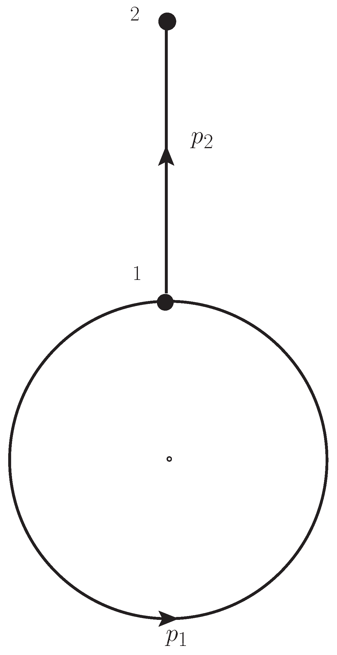
In the perturbation expansion, the tadpole diagram (Figure 1) appears as a propagator with both ends attached to the same vertex, which is the (lower-time) end-point vertex of the second propagator.

The tadpole subdiagram without a leg is simple. Of the three components, the loop integral vanishes for the R and A components and diverges for the $K,R$ and $K,A$ ones. At finite $\kappa =4-d$, these integrals are real constants related to the F and $\overline{F}$ components. In the limit $d=4$, the renormalization performed on F and $\overline{F}$ makes them finite.

$$\begin{array}{c}ig{\mu }^{\kappa /2}\frac{\int d^{d}p}{{(2\pi )}^d}{G}_R(p)=ig{\mu }^{\kappa /2}\frac{\int d^{d}p}{{(2\pi )}^d}{G}_A(p)=0,\hfill \\ G_{Tad}\equiv -ig\frac{\int d^{4}p}{{(2\pi )}^4}{G}_{K,A}(p)=-ig{\mu }^{\kappa /2}\frac{\int d^{d}p}{{(2\pi )}^d}\frac{p_0}{{\omega }_p}\frac{1+2f({\omega }_p)}{p^2-m^2-2i{p}_0ϵ}=ig{\mu }^{\kappa /2}\frac{\int d^{d}p}{{(2\pi )}^d}{G}_{K,R}(p),\hfill \\ ⟹-\frac{1}{2}{G}_{Tad}=-\frac{ig{m}^2}{8{\pi }^2\kappa }-\frac{ig{m}^2}{16{\pi }^2}[1-{\gamma }_{{}_E}+ln(\frac{4\pi {\mu }^2}{m^2})]+\mathcal{O}(\kappa )+ig\frac{\int d^{3}p}{{(2\pi )}^3}2f({\omega }_p)\hfill \\ =-\frac{ig{m}^2}{8{\pi }^2(\kappa )}+finitevacuumterm+finitef({\omega }_p)term.\hfill \end{array}$$

(5)

(Above, and throughout the paper, ${\gamma }_{{}_E}$ denotes the Euler-Mascheroni constant, ${\gamma }_{{}_E}\approx 0.5772$.)

For a tadpole subdiagram with a leg (see Figure 1), we have two vertices; higher in time ($t_2$), which is the connection to the rest of the diagram, and lower in time ($t_1,t_1<t_2$) with the tadpole loop. The lower vertex does not conserve energy.

One has to add contributions from vertices of Type 1 and Type 2. We write it symbolically with the help of the Wigner transform, the connection between the Keldysh-time-path propagators and the finite-time-path propagators at the time $t^{\prime }=\infty$ and transition to the $R/A$ basis. The derivation given in the Appendix A shows that:

$$G_{tad,j}(x_2)=-G_A(0,0)G_{Tad}+\int \frac{d{p}_{02}}{2\pi }\frac{i{e}^{i{p}_{02}{x}_{02}}}{p_{02}-iϵ}[G_A(p_{02},0)-G_A(0,0)]G_{Tad}.$$

(6)

The contribution is split into the first, energy-conserving term, and the second term, oscillating with time, in which energy is not conserved at the vertex 1 [31].

The tadpole counterterm follows the same pattern:

$$G_{count,j}^{tadpole}(x_2)=-G_A(0,0)+\int \frac{d{p}_{02}}{2\pi }\frac{i{e}^{i{p}_{02}{x}_{02}}}{p_{02}-iϵ}[G_A(p_{02},0)-G_A(0,0)].$$

(7)

Notice the similarity of the expressions (6) and (7).

An important point here is that the tadpole contribution splits into two: (1) the energy-conserving part and (2) the energy nonconserving part.

In the energy conserving part, the constant multiplying the counterterm may be adjusted to satisfy the renormalization condition $\langle 0\left|\varphi \right|0\rangle =0$ of the S-matrix theory, by which the tadpoles are completely eliminated from perturbation expansion. Nevertheless, the terms proportional to f survive. The energy nonconserving terms oscillate with time, with the frequency depending on the energy increment. In the competition with the contributions of subdiagram without tadpoles, they fade with time, thus giving the same $t\to \infty$ limit as expected from S-matrix theory.

The $g^3$ order tadpoles and tadpoles with the resummed loop propagator (obtainable after renormalizing the self-energy; see further in the text) do not change our conclusions.

2.3. UV Divergence at the Self-Energy Subdiagram

While in the S-matrix theory, there is only Feynman (${\Sigma }_F^1(p_0,\overrightarrow{p})$) one-loop self energy, which does not depend on the frame, in out-of-equilibrium FT, we have self-energies ${\Sigma }_R^1(p_0,\overrightarrow{p})$, ${\Sigma }_A^1(p_0,\overrightarrow{p})$, and ${\Sigma }_K^1(p_0,\overrightarrow{p})$, which is frame dependent through $f({\omega }_p)$ (notice here that we distinguish the “true” retarded and advanced functions from those that carry index R (A), but do not vanish for $t_2>t_1$ ($t_2<t_1$), except at $d<4$).

$${\Sigma }_R^1(p_0,\overrightarrow{p})=-i{g}^2{\mu }^{\kappa }\int \frac{d^{d}q}{2{(2\pi )}^d}[G_R(p_0-q_0,\overrightarrow{p}-\overrightarrow{q})G_{K,R}(q_0,\overrightarrow{q})$$

$$+G_{K,R}(p_0-q_0,\overrightarrow{p}-\overrightarrow{q})G_R(q_0,\overrightarrow{q})]={\Sigma }_A^{1,*}(p_0,\overrightarrow{p}),$$

$${\Sigma }_K^1(p_0,\overrightarrow{p})=-{\Sigma }_{K,R}^1(p_0,\overrightarrow{p})+{\Sigma }_{K,A}^1(p_0,\overrightarrow{p})$$

(8)

$${\Sigma }_{K,R}^1(p_0,\overrightarrow{p})=-i{g}^2{\mu }^{\kappa }\int \frac{d^{d}q}{2{(2\pi )}^d}[G_{K,R}(p_0-q_0,\overrightarrow{p}-\overrightarrow{q})G_{K,R}(q_0,\overrightarrow{q})$$

$$+G_R(p_0-q_0,\overrightarrow{p}-\overrightarrow{q})q,G_R(q_0,\overrightarrow{q})]=-{\Sigma }_{K,A}^{1,*}(p_0,\overrightarrow{p}).$$

(9)

Now, all the integrals containing $f({\omega }_p)$ are UV finite owing to the assumed UV cut-off in the definition of f. Vacuum contributions to ${\Sigma }_{K,R}^1$ are finite separately at $d\to 4$; at $d\to 6$, this is no longer the case, but their sum is finite.

For retarded and advanced self-energies, imaginary parts and parts proportional to $f({\omega }_p)$ are UV finite and could be calculated directly from (8). Real, vacuum parts of ${\Sigma }_R^1$ are connected to ${\Sigma }_F^1$, and we use the results already available from S-matrix renormalization. The connection is:

$${\Sigma }_{j,k}^1=\frac{1}{2}[-{\Sigma }_{K,R}^1+{\Sigma }_{K,A}^1-{(-1)}^k{\Sigma }_R^1-{(-1)}^j{\Sigma }_A^1],$$

$$Re{\Sigma }_{R,f=0}^1=Re{\Sigma }_{11}^1+{\Sigma }_{K,R,f=0}^1={\Sigma }_F^1+{\Sigma }_{K,R,f=0}^1.$$

(10)

The regularization procedure (either by making $d<4$ or by introducing fictive massive particles as in Pauli–Villars regularization) is usually considered artificial. Nevertheless, there are efforts to generate necessary massive particles (virtual wormholes) dynamically [32].

For ${\Sigma }_F^1(p)$, we find in the literature [33]:

$$\begin{array}{c}{\Sigma }_F^1(p)=\frac{1}{2}{i}^2{g}^2\frac{\int d^4{q}_1{d}^4{q}_2}{{(2\pi )}^8}{G}_F(q_1)G_F(q_2){(2\pi )}^4{\delta }^{(4)}(q_1-q_2-p),\hfill \\ =\frac{1}{2}{g}^2\frac{\int d^4{q}_1{d}^4{q}_2}{{(2\pi )}^8}\frac{{(2\pi )}^4{\delta }^{(4)}(q_1-q_2-p)}{(q_1^2-m^2+iϵ)(q_2^2-m^2+iϵ)},\hfill \\ ⟹\frac{1}{2}{g}^2{(\mu )}^{\kappa }{\int }_0^{1}dz\int \frac{d^d{q}^{\prime }}{{(2\pi )}^d}\frac{1}{{[q^{\prime 2}-m^2+p^{2}z(1-z)+iϵ]}^2},\hfill \\ =\frac{i{g}^2}{32{\pi }^2}{({\mu }^2)}^{\kappa /2}\Gamma (\kappa /2){\int }_0^{1}dz{[\frac{p^{2}z(1-z)-m^2+iϵ}{4\pi {\mu }^2}]}^{-\kappa /2}.\hfill \end{array}$$

(11)

The last relation above is still causal. It is UV finite, and it allows the separation into the sum of the retarded and advanced term. However, the expansion of ${[p^{2}z(1-z)-m^2+iϵ/4\pi {\mu }^2]}^{-\kappa /2}$ in power series of $\left|\kappa \right|$ is allowed only when $\kappa ln[p^2/(4\pi \mu )]<<1$; thus, it is a “low energy” expansion, and in spite of the fact that $\kappa$ may be taken arbitrarily small, the limit $|p_0|\to \infty$ is never allowed.

$$\begin{array}{c}{\Sigma }_F^1(p)\approx \frac{i{g}^2{\mu }^{\kappa }}{16{\pi }^2(\kappa )}-\frac{i{g}^2{\mu }^{\kappa }}{32{\pi }^2}[{\gamma }_{{}_E}+{\int }_0^{1}dzln[\frac{p^{2}z(1-z)-m^2+iϵ}{4\pi {\mu }^2}]]\hfill \\ =\frac{i{g}^2{\mu }^{\kappa }}{16{\pi }^2(\kappa )}+finite.\hfill \end{array}$$

(12)

This expression is no longer causal; it is valid only if $\kappa ln[p^2/(4\pi \mu )]<<1$. One needs the vanishing of self-energy for $|p_0|\to \infty$, i.e., the region where the opposite condition $\kappa ln[p^2/(4\pi \mu )]>>1$ is fulfilled. Then, $|{\Sigma }_{\infty ,F}^1(p)|\to 0$ as $|p_0|\to \infty$ as far as $\kappa \ne 0$.

The integration over z gives:

$${\Sigma }_F^1(p)=-\frac{g^2}{16{\pi }^2}\left\{\frac{1}{\kappa }-\frac{{\gamma }_{{}_E}}{2}+1+\frac{1}{2}ln(4\pi \frac{{\mu }^2}{m^2})-\frac{1}{2}\sqrt{1-\frac{4m^2}{p^2+iϵ}}ln\left[\frac{\sqrt{1-\frac{4m^2}{p^2+iϵ}}+1}{\sqrt{1-\frac{4m^2}{p^2+iϵ}}-1}\right]\right\}$$

(13)

with a high $p_0$ limit:

$${\Sigma }_F{(p^2,m^2)}_{p^2\to \infty }\approx -\frac{g^2}{16{\pi }^2}\left\{\frac{1}{\kappa }-\frac{{\gamma }_{{}_E}}{2}+1+\frac{1}{2}ln(4\pi \frac{{\mu }^2}{m^2})-\frac{1}{2}ln\left[-\frac{m^2}{p^2}\right]\right\}.$$

(14)

To verify the causality of the two-point function, one may try to project out the retarded part of the finite (subtracted) part of ${\Sigma }_F^1(p)$, namely $-i\int \frac{d{p}_0^{\prime }}{2\pi }{\Sigma }_{F,finite}^1(p)/(p_0-p_0^{\prime }-iϵ)$, by integration $\int d{p}_0$ over a large semicircle. However, the contribution over a very large semicircle does not vanish, and the integral is ill defined.

Indeed, we have started from the expressions for $G_F$ (${\Sigma }_F$) containing only retarded and advanced functions, and in the absence of divergence, we expect this to be the truth at the end of calculation. Instead, the function in the last two lines of Expression (12) is not a combination of the R and A functions, otherwise it should vanish when $|p_0|\to \infty$ and $\kappa$ are chosen as arbitrarily small; such a behavior can be shifted to an arbitrarily high scale. However, the limit $\kappa \to 0$ remains always out of reach. To preserve causality, we should keep the whole $p_0$ complex plane. Specifically, we need the region with large $|p_0|$, to be able to integrate over a large semicircle in the complex $p_0$ plane, at least to get $\int d{p}_0{\Sigma }_R^1(p)G_{K,A}(p_0)=0$. Thus, we have obtained a result correct at $\kappa \ne 0$ and problematic at $d=4$.

Fortunately enough, there is a way to “repair” causality: the composite object $G_F(p){\Sigma }_F^1(p)$ is vanishing when $|p_0|\to \infty$; it can be split into its retarded and advanced parts; thus, it is causal. This sort of reparation of causality is possible in other QFT in which logarithmic UV divergence appears. It is similar to the Glaser–Epstein [34,35,36] approach, where not just $\Sigma$, but $G\Sigma$ are the subjects of expansion.

In this spirit, we agree with the conclusion of [37,38,39]: “Our amplitudes are manifestly causal, by which we mean that the source and detector are always linked by a connected chain of retarded propagators.”

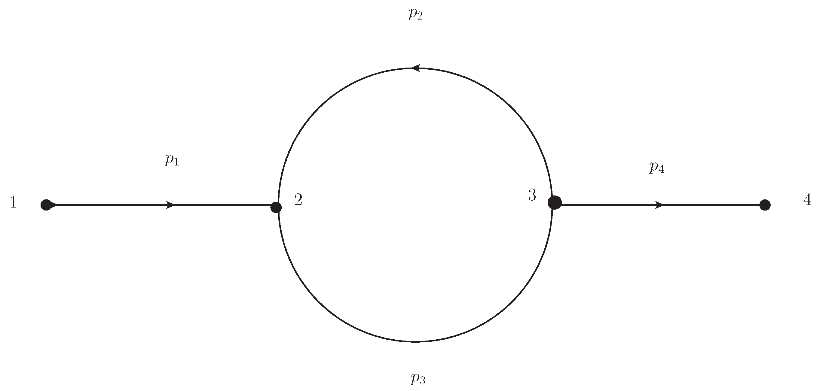
Similar is the problem we can see by considering $\lambda {\varphi }^4$ theory. In this theory, the loop of Figure 2 is a vertex diagram, and the above Glaser–Epstein philosophy does not apply. Nevertheless, the propagator attached to the vertex depends on $p_0$ and “improves” the convergence of $d{p}_0$ integration.

2.4. Self-Energy Diagram with Legs

To be able to introduce composite objects with ${\Sigma }_{R(A)}$, we need one of ${\Sigma }_{R(A)}$’s vertices to conserve energy. The lower in time vertex may be the minimal time vertex, so it does not help in all cases. However, the higher in time vertex would do it, if both the integrals $d{q}_0$ and $d{p}_0$ converge.

The ${\Sigma }_{ij}$ self-energy contributions with legs (see Figure 2) are:

$$G_R{\Sigma }_{K,R}^1\ast G_A,G_R\ast {\Sigma }_{K,A}^1{G}_A,G_R{\Sigma }_R^1\ast G_{K,A},G_{K,R}\ast {\Sigma }_A^1{G}_A,$$

$$G_R{\Sigma }_R^1\ast G_A,G_A{\Sigma }_A^1{G}_A,G_R{\Sigma }_R^1{G}_{K,R},G_{K,A}{\Sigma }_A^1{G}_A.$$

(15)

In the above expression, $\Sigma$s are introduced in Equation (8). “∗” indicates the convolution product, which includes the energy nonconserving vertex. Terms containing ${\Sigma }_{K,R}^1$ and ${\Sigma }_{K,A}^1$ are UV-finite, creating no problems. The other terms, containing ${\Sigma }_R^1$ and ${\Sigma }_A^1$, are finite as long as $d<4$, and we may obtain their real part through (11).

Two features seem potentially suspicious: (1) UV divergence in the loop defining ${\Sigma }_{R(A)}^1$, (2) the ill-defined vertex function between $G_R$ and ${\Sigma }_R^1$ and between ${\Sigma }_A^1$ and $G_A$.

Nevertheless, both problems are resolved at $d<4$: “to be” UV divergence is subtracted and energy conservation is recovered in the above-mentioned vertices. The composite objects $G_R(p){\Sigma }_R^1(p)$ and ${\Sigma }_A^1(p)G_{FA}(p)$ are now well defined.

3. Discussion and Conclusions

We examined renormalization prescriptions for the finite-time-path out-of-equilibrium $\lambda {\varphi }^3$ QFT in the basis of $G_R,G_A,G_{K,R}$, and $G_{K,A}$ propagators.

As expected, the number of counterterms did not change, and the formalism enables term by term finite perturbation calculation.

There are some interesting features:

• The integrals ensuring the energy conservation at the vertices above ${\Sigma }_R$ and ${\Sigma }_A$ should have been done before taking the limit $d=4$.
• The renormalized self-energies (${\Sigma }_F$, ${\Sigma }_R$, and ${\Sigma }_A$) are not a linear combination of true retarded and advanced components. This is directly readable from the final result, which does not vanish as $|p_0|\to \infty$ in all directions in a complex plane $p_0$. This problem is present already in S-matrix theory, and we only recognize it properly as a causality problem, in the sense that the expected properties of the theta-function fail: $\Theta (t)\Theta (-t)\ne 0$ or $\Theta (t)\Theta (t)\ne \Theta (t)$. While it is not clear what harm it does to the theory, one may introduce “composite objects” $G_F(p){\Sigma }_F^1(p)$, $G_R(p){\Sigma }_R^1(p)$, and ${\Sigma }_A^1(p)G_A(p)$ to improve convergence, and the causality is “repaired”. Indeed in the Glaser–Epstein approach, they consider the perturbation expansion, in which only self-energy with a leg appears.
• The tadpole contribution splits into the energy-conserving, constant component, which is eliminated by renormalization condition, and the other energy nonconserving, time-dependent component, is finite after subtraction. These tadpole contributions are strongly oscillating with time and vanish as $t\to \infty$, in good agreement with the renormalization condition $<0\left|\varphi \right|0>=0$ of the S-matrix theory.
• The regularization ($d\ne 4$) is extended till the late phase of calculation.

The procedure is therefore generalized for application to more realistic theories (QED and QCD, electro-weak QFT, etc.) by the following:

(A) regularize; (B) do energy-conserving integrals; (C) subtract “to be” UV infinities; (D) deregularize (do limit $d\to 4$).

Again, the above described Features (1) and (2) will emerge.

This work contains many of the features [40] arising in the more realistic theories like QED or QCD. Such finite-time-path renormalization is a necessary prerequisite for the calculation of damping rates, and other transition coefficients under the more realistic conditions truly away from equilibrium as opposed to the results obtained within the linear response approximation.

Our plan is to extend the exposed methods to the case of QED. Specifically, we resolve the controversy of the UV diverging number of direct photons in the lowest order of quark QED, as calculated by Boyanovsky and collaborators [41,42] and criticized by [43]. We find that, at the considered one-loop order of perturbation, it is only the vacuum-polarization diagram contributing. The renormalization leaves only finite contributions to the photon production [44].

References

- Bollini, C.G.; Giambiagi, J.J. Dimensional Renormalization: The Number of Dimensions as a Regularizing Parameter. Nuovo Cim. B 1972, 12, 20–26. [Google Scholar]
- ’t Hooft, G.; Veltman, M.J.G. Regularization and Renormalization of Gauge Fields. Nucl. Phys. B 1972, 44, 189. [Google Scholar] [CrossRef]
- Ashmore, J.F. A Method of Gauge Invariant Regularization. Nuovo Cim. Lett. 1972, 4, 289. [Google Scholar] [CrossRef]
- Cicuta, G.M.; Montaldi, E. Analytic renormalization via continuous space dimension. Nouvo Cim. Lett. 1972, 4, 329. [Google Scholar] [CrossRef]
- Wilson, K.G. Quantum field theory models in less than four-dimensions. Phys. Rev. D 1973, 7, 2911. [Google Scholar] [CrossRef]
- Donoghue, J.F.; Holstein, B.R. Renormalization and Radiative Corrections at Finite Temperature. Phys. Rev. D 1983, 28, 340. [Google Scholar] [CrossRef]
- Donoghue, J.F.; Holstein, B.R. Renormalization and Radiative Corrections at Finite Temperature, Erratum. Phys. Rev. D 1984, 29, 3004. [Google Scholar] [CrossRef]
- Chapman, I.A. Finite temperature wave function renormalization: A Comparative analysis. Phys. Rev. D 1997, 55, 6287–6291. [Google Scholar] [CrossRef]
- Nakkagawa, H.; Yokota, H. Effective potential at finite temperature: RG improvement versus high temperature expansion. Prog. Theor. Phys. Suppl. 1997, 129, 209–214. [Google Scholar] [CrossRef]
- Baacke, J.; Heitmann, K.; Patzold, C. Renormalization of nonequilibrium dynamics at large N and finite temperature. Phys. Rev. D 1998, 57, 6406–6419. [Google Scholar] [CrossRef] [Green Version]
- Esposito, S.; Mangano, G.; Miele, G.; Pisanti, O. Wave function renormalization at finite temperature. Phys. Rev. D 1998, 58, 105023. [Google Scholar] [CrossRef] [Green Version]
- van Hees, H.; Knoll, J. Renormalization in selfconsistent approximation schemes at finite temperature. 3. Global symmetries. Phys. Rev. D 2002, 66, 025028. [Google Scholar] [CrossRef]
- Jakovac, A.; Szep, Z. Renormalization and resummation in finite temperature field theories. Phys. Rev. D 2005, 71, 105001. [Google Scholar] [CrossRef]
- Arrizabalaga, A.; Reinosa, U. Renormalized finite temperature phi**4 theory from the 2PI effective action. Nucl. Phys. A 2007, 785, 234–237. [Google Scholar] [CrossRef]
- Blaizot, J.-P.; Ipp, A.; Mendez-Galain, R.; Wschebor, N. Perturbation theory and non-perturbative renormalization flow in scalar field theory at finite temperature. Nucl. Phys. A 2007, 784, 376–406. [Google Scholar] [CrossRef] [Green Version]
- Blaizot, J.-P.; Wschebor, N. Massive renormalization scheme and perturbation theory at finite temperature. Phys. Lett. B 2015, 741, 310–315. [Google Scholar] [CrossRef] [Green Version]
- Schwinger, J. Brownian motion of a quantum oscillator. J. Math. Phys. 1961, 2, 407. [Google Scholar] [CrossRef]
- Keldysh, L.V. Diagram technique for nonequilibrium processes. ZH. Eksp. Teor. Fiz. 1964, 47, 1515. [Google Scholar]
- Kadanoff, L.P.; Baym, G. Quantum Statistical Mechanics; Benjamin: New York, NY, USA, 1962. [Google Scholar]
- Danielewicz, P. Quantum Theory Of Nonequilibrium Processes. Ii. Application To Nuclear Collisions. Ann. Phys. 1984, 152, 239. [Google Scholar] [CrossRef]
- Rammer, J.; Smith, H. Quantum field-theoretical methods in transport theory of metals. Rev. Math. Phys. 1986, 58, 323. [Google Scholar] [CrossRef]
- Landsman, N.P.; van Weert, C.G. Real and Imaginary Time Field Theory at Finite Temperature and Density. Phys. Rep. 1987, 145, 141. [Google Scholar] [CrossRef]
- Calzetta, E.; Hu, B.L. Nonequilibrium Quantum Fields: Closed Time Path Effective Action, Wigner Function and Boltzmann Equation. Phys. Rev. D 1988, 37, 2878. [Google Scholar] [CrossRef]
- le Bellac, M. Thermal Field Theory; Cambridge University Press: Cambridge, UK, 1996. [Google Scholar]
- Brown, D.A.; Danielewicz, P. Partons in phase space. Phys. Rev. D 1998, 58, 094003. [Google Scholar] [CrossRef] [Green Version]
- Blaizot, J.-P.; Iancu, E. The Quark gluon plasma: Collective dynamics and hard thermal loops. Phys. Rept. 2002, 359, 355–528. [Google Scholar] [CrossRef]
- Dadić, I. Out-of-equilibrium thermal field theories: Finite time after switching on the interaction: Fourier transforms of the projected functions. Phys. Rev. D 2001, 63, 025011. [Google Scholar] [CrossRef]
- Dadić, I. Erratum: Out of equilibrium thermal field theories: Finite time after switching on the interaction and Wigner transforms of projected functions. Phys. Rev. D 2002, 66, 069903. [Google Scholar] [CrossRef]
- Dadić, I. Out-of-equilibrium thermal field theories: Finite time after switching on the interaction: Fourier transforms of the projected functions, Erratum. Nucl. Phys. A 2002, 702, 356. [Google Scholar] [CrossRef]
- Bedaque, P.F. Thermalization and pinch singularities in nonequilibrium quantum field theory. Phys. Lett. B 1995, 344, 23. [Google Scholar] [CrossRef]
- Dadić, I. Retarded propagator representation of out-of-equilibrium thermal field theories. Nucl. Phys. A 2009, 820, 267C–270D. [Google Scholar] [CrossRef]
- Kirillov, A.A.; Savelova, E.P. On the possible dynamical realization of the Pauli–Villars regularization. Phys. Atom. Nucl. 2015, 78, 1069. [Google Scholar] [CrossRef]
- Ryder, L.H. Quantum Field Theory; Cambridge University Press: Cambridge, UK, 1985. [Google Scholar]
- Epstein, H.; Glaser, V. The Role of locality in perturbation theory. Ann. Inst. Henri Poincare Phys. Theor. A 1973, 19, 211. [Google Scholar]
- Scharf, G. Finite Quantum Electrodynamics—The Causal Approach; Springer: Berlin/Heidelberg, Germany, 1995. [Google Scholar]
- Lazzarini, S.; Gracia-Bondıa, J.M. Improved Epstein-Glaser renormalization in coordinate space. 1. Euclidean framework. J. Math. Phys. 2003, 44, 3863. [Google Scholar] [CrossRef]
- Millington, P.; Pilaftsis, A. Perturbative Non-Equilibrium Thermal Field Theory to all Orders in Gradient Expansion. Phys. Lett. B 2013, 724, 56–62. [Google Scholar] [CrossRef]
- Millington, P.; Pilaftsis, A. Perturbative nonequilibrium thermal field theory. Phys. Rev. D 2013, 88, 085009. [Google Scholar] [CrossRef]
- Dickinson, R.; Forshaw, J.; Millington, P.; Cox, B. Manifest Causality in quantum field theory with sources and detectors. JHEP 2014, 1406, 049. [Google Scholar] [CrossRef]
- Urmossy, K.; Xu, Z. PoS DIS 2016, 265, 054.
- Wang, S.-Y.; Boyanovsky, D. Enhanced photon production from quark—gluon plasma: Finite lifetime effect. Phys. Rev. D 2001, 63, 051702. [Google Scholar] [CrossRef]
- Wang, S.-Y.; Boyanovsky, D.; Ng, K.-W. Direct photons: A nonequilibrium signal of the expanding quark gluon plasma at RHIC energies. Nucl. Phys. A 2002, 699, 819–846. [Google Scholar] [CrossRef]
- Arleo, F.; Aurenche, P.; Bopp, F.; Dadic, I.; David, G.; Delagrange, H.; d’Enterria, D.; Eskola, K.J.; Gelis, F.; Guillet, J.-Ph.; et al. Photon Physics in Heavy Ion Collisions at the LHC. 2004. Available online: http://cds.cern.ch/record/815045 (accessed on 30 November 2018).
- Dadić, I.; Klabučar, D.; Kuić, D. Direct Photons from Hot Quark Matter in Renormalized Finite-Time-Path QED, (unpublished).
Figure 1.
The tadpole diagram with a leg.
Figure 2.
The vertex diagram.
© 2019 by the authors. Licensee MDPI, Basel, Switzerland. This article is an open access article distributed under the terms and conditions of the Creative Commons Attribution (CC BY) license (http://creativecommons.org/licenses/by/4.0/).
Share and Cite
MDPI and ACS Style
Dadić, I.; Klabučar, D. Causality and Renormalization in Finite-Time-Path Out-of-Equilibrium ϕ3 QFT. Particles 2019, 2, 92-102. https://doi.org/10.3390/particles2010008
AMA Style
Dadić I, Klabučar D. Causality and Renormalization in Finite-Time-Path Out-of-Equilibrium ϕ3 QFT. Particles. 2019; 2(1):92-102. https://doi.org/10.3390/particles2010008
Chicago/Turabian StyleDadić, Ivan, and Dubravko Klabučar. 2019. "Causality and Renormalization in Finite-Time-Path Out-of-Equilibrium ϕ3 QFT" Particles 2, no. 1: 92-102. https://doi.org/10.3390/particles2010008