Author Contributions
Conceptualization and Methodology, D.A.X., T.N.A., A.B. and E.S.V.; validation, T.N.A. and E.S.V.; formal analysis, D.A.X., T.N.A. and A.B.; writing—original draft preparation, T.N.A.; writing—review and editing, M.U.G., M.I. and T.N.A.; visualization, M.U.G. and M.I.; supervision, D.A.X. All authors have read and agreed to the published version of the manuscript.
Figure 1.
(a) Molecular graph of , (b) Molecular graph of .
Figure 1.
(a) Molecular graph of , (b) Molecular graph of .
Figure 2.
(a) 2-D lattice of , (b) 2-D lattice of .
Figure 2.
(a) 2-D lattice of , (b) 2-D lattice of .
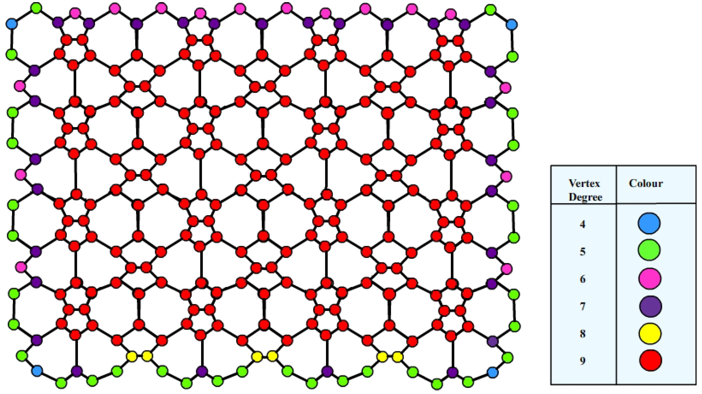
Figure 3.
Neighborhood degree illustration of .
Figure 3.
Neighborhood degree illustration of .
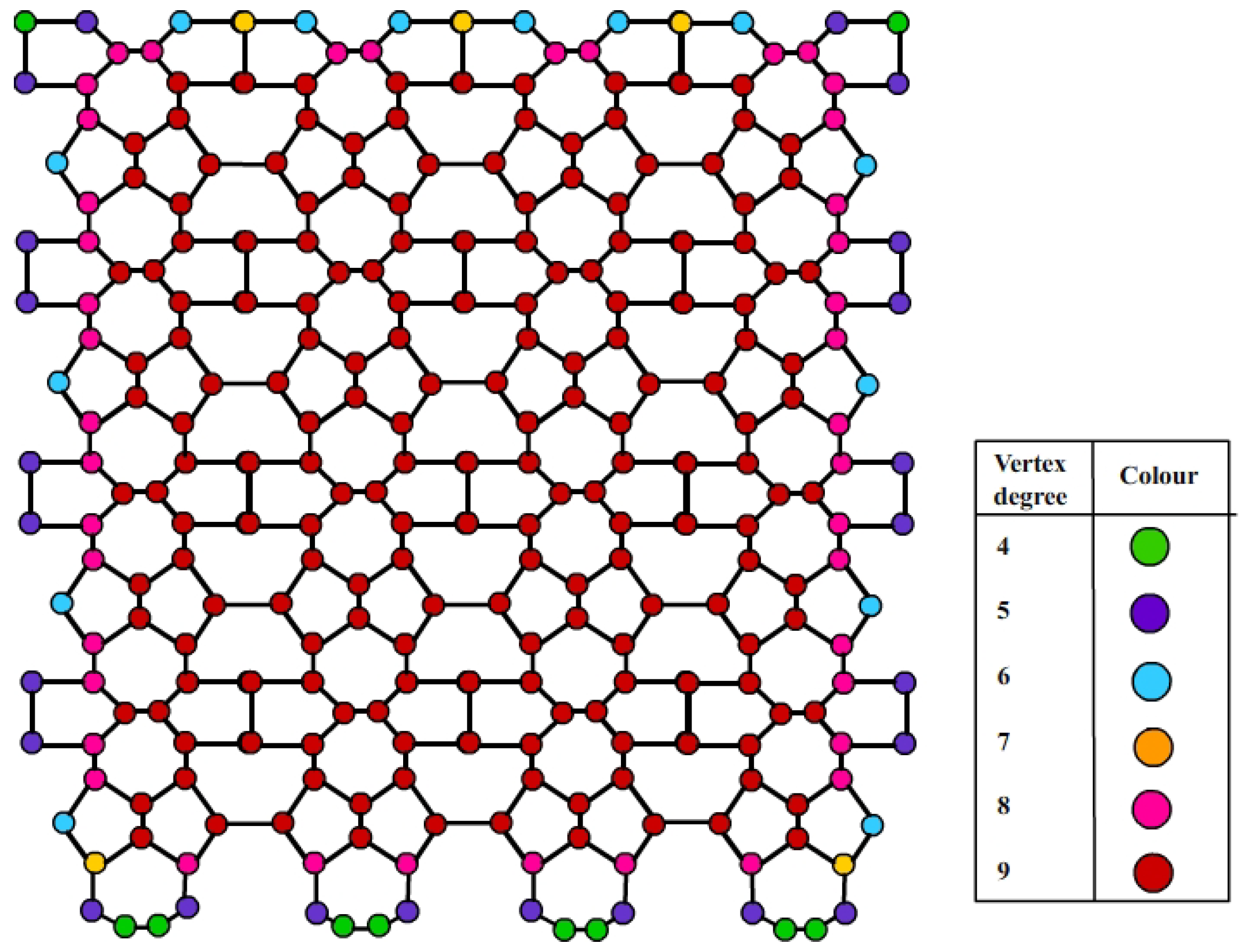
Figure 4.
Neighborhood degree illustration of .
Figure 4.
Neighborhood degree illustration of .
Figure 5.
Flowchart relating Topological Descriptors and its potential uses.
Figure 5.
Flowchart relating Topological Descriptors and its potential uses.
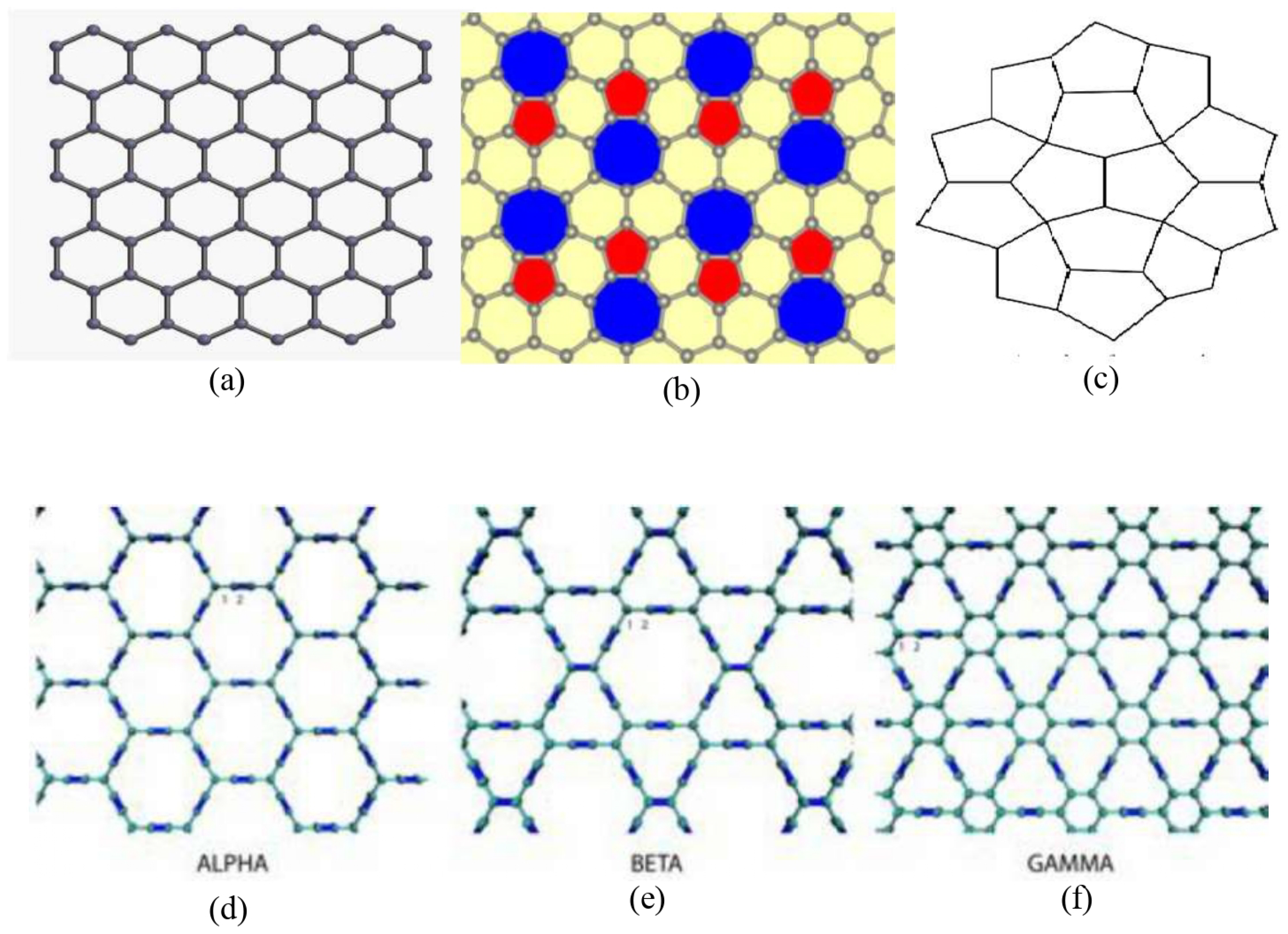
Figure 6.
Graphene and its derivatives; (a) Graphene (b) Phagraphene (c) Penta Graphene (d) graphyne (e) graphyne (f) graphyne.
Figure 6.
Graphene and its derivatives; (a) Graphene (b) Phagraphene (c) Penta Graphene (d) graphyne (e) graphyne (f) graphyne.
Figure 7.
Scatter Diagram for the properties.
Figure 7.
Scatter Diagram for the properties.
Figure 8.
The NM polynomial graph of (a) and (b) .
Figure 8.
The NM polynomial graph of (a) and (b) .
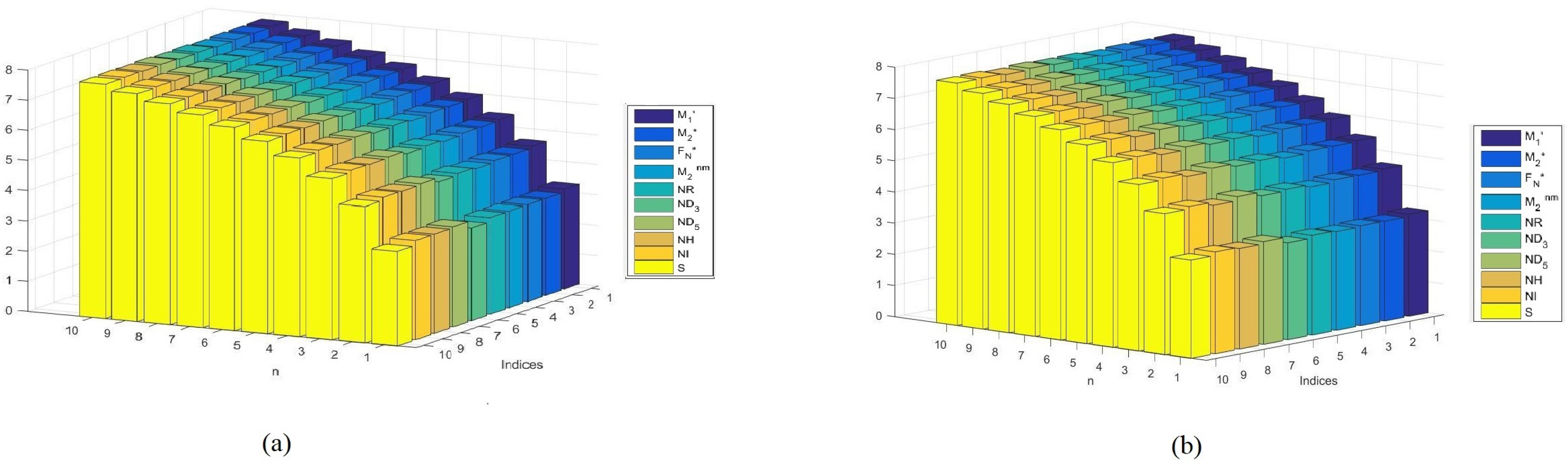
Figure 9.
The neighborhood degree indices of .
Figure 9.
The neighborhood degree indices of .
Figure 10.
The neighborhood degree indices of .
Figure 10.
The neighborhood degree indices of .
Figure 11.
Comparison graph of neighborhood general Randic index of and at .
Figure 11.
Comparison graph of neighborhood general Randic index of and at .
Figure 12.
Comparison graph of neighborhood entropy measures (a) and (b) .
Figure 12.
Comparison graph of neighborhood entropy measures (a) and (b) .
Table 1.
A few of the neighborhood degree-based descriptors.
Table 1.
A few of the neighborhood degree-based descriptors.
| Topological Index | | Derivation from |
|---|
| | |
| | |
| | |
| | |
| | |
| | |
| | |
| | |
| | |
| S | | |
Table 2.
Edge partition of .
Table 2.
Edge partition of .
| Edge Partition | Number of Edges | Edge Set |
|---|
| 8 | |
| | |
| | |
| | |
| | |
| | |
| | |
| | |
| | |
Table 3.
Edge partition of .
Table 3.
Edge partition of .
| Edge Partition | Number of Edges | Edge Set |
|---|
| b | |
| | |
| | |
| 2 | |
| | |
| | |
| | |
| | |
| | |
| | |
| | |
Table 4.
Experimental Results for Young’s Modulus and Poisson’s Ratio of Graphene Derivatives.
Table 4.
Experimental Results for Young’s Modulus and Poisson’s Ratio of Graphene Derivatives.
| Sl No. | Name | Young’s Modulus (N/m) | Poisson’s Ratio |
|---|
| 1 | Graphene | 348 | 0.456 |
| 2 | Penta Graphene | 277.99 | −0.078 |
| 3 | Phagraphene | 292.92 | 0.255 |
| 4 | graphyne | 21.98 | 0.87 |
| 5 | graphyne | 73.07 | 0.67 |
| 6 | graphyne | 165.51 | 0.42 |
| 7 | Penta heptite graphene | 292.26 | 0.253 |
Table 5.
Computed numerical values of neighborhood descriptors for the base structures of graphene allotropes.
Table 5.
Computed numerical values of neighborhood descriptors for the base structures of graphene allotropes.
| Sl No. | Name | | | | | | | |
|---|
| 1 | Graphene | 100.63 | 4.6167 | 408 | 0.75217 | 1434 | 21,336 | 61.752 |
| 2 | Penta Graphene | 74.495 | 2.719 | 300 | 0.37919 | 1140 | 17,790 | 40.556 |
| 3 | Phagraphene | 115.52 | 5.1605 | 468 | 0.82801 | 1662 | 24,894 | 69.863 |
| 4 | Graphyne | 214.85 | 19.112 | 864 | 4.155 | 2100 | 20,880 | 181.8 |
| 5 | Graphyne | 168.67 | 13.224 | 684 | 2.7732 | 1812 | 20,160 | 135.34 |
| 6 | Graphyne | 145.22 | 10.312 | 588 | 2.0587 | 1650 | 19,632 | 110.55 |
| 7 | Pentaheptite Graphene | 89.76 | 4.6 | 364 | 0.81728 | 1244 | 18,222 | 57.679 |
Table 6.
Correlation table for the properties for various neighborhood degree descriptors.
Table 6.
Correlation table for the properties for various neighborhood degree descriptors.
| Sl No. | Descriptors | Young’s Modulus (N/m) | Poisson’s Ratio |
|---|
| 1 | NI | −0.918698 | 0.916982 |
| 2 | NH | −0.948272 | 0.895635 |
| 3 | | −0.918348 | 0.918611 |
| 4 | | −0.952106 | 0.889633 |
| 5 | | −0.803185 | 0.909173 |
| 6 | | 0.214892 | 0.185452 |
| 7 | | −0.940875 | 0.907696 |
Table 7.
Computed numerical values for the NM polynomial function.
Table 7.
Computed numerical values for the NM polynomial function.
| Sl No. | | | |
|---|
| 1 | (−3,−3) | 108,259,334,352 | 93,460,421,484 |
| 2 | (−2,−2) | 73,990,144 | 62,284,800 |
| 3 | (−1,−1) | 296 | 224 |
| 4 | (0,0) | 0 | 0 |
| 5 | (1,1) | 400 | 396 |
| 6 | (2,2) | 76,193,792 | 74,322,944 |
| 7 | (3,3) | 109,930,499,784 | 104,920,887,600 |
Table 8.
Computed numerical values for the neighborhood indices of .
Table 8.
Computed numerical values for the neighborhood indices of .
| a | | | | S | | | | | |
|---|
| 1 | 364 | 1244 | 2550 | 1745.272433 | 18,222 | 0.817283951 | 4.60 | 57.67936508 | 89.76014957 |
| 2 | 1584 | 6249 | 12,646 | 9402.205206 | 102,472 | 2.138058862 | 14.38 | 211.5888889 | 393.1922763 |
| 3 | 3668 | 15,142 | 30,518 | 23,286.9622 | 256,706 | 4.051426367 | 29.50 | 461.4984127 | 912.624403 |
| 4 | 6616 | 27,923 | 56,166 | 43,399.54341 | 480,924 | 6.557386464 | 49.95 | 807.4079365 | 1648.05653 |
| 5 | 10,428 | 44,592 | 89,590 | 69,739.94884 | 775,126 | 9.655939153 | 75.74 | 1249.31746 | 2599.488656 |
| 6 | 15,104 | 65,149 | 130,790 | 102,308.1785 | 1,139,312 | 13.34708444 | 106.85 | 1787.226984 | 3766.920783 |
| 7 | 20,644 | 89,594 | 179,766 | 141,104.2324 | 1,573,482 | 17.63082231 | 143.30 | 2421.136508 | 5150.35291 |
| 8 | 27,048 | 117,927 | 236,518 | 186,128.1104 | 2,077,636 | 22.50715278 | 185.09 | 3151.046032 | 6749.785036 |
| 9 | 34,316 | 150,148 | 301,046 | 237,379.8127 | 2,651,774 | 27.97607584 | 232.21 | 3976.955556 | 8565.217163 |
| 10 | 42,448 | 186,257 | 373,350 | 294,859.3393 | 3,295,896 | 34.03759149 | 284.66 | 4898.865079 | 10,596.64929 |
Table 9.
Computed numerical values for the neighborhood indices of .
Table 9.
Computed numerical values for the neighborhood indices of .
| a | | | | S | | | | | |
|---|
| 1 | 356 | 1217 | 2504 | 1687.166041 | 17,606 | 0.75892306 | 4.346863104 | 55.79761905 | 87.63862853 |
| 2 | 1572 | 6242 | 12,654 | 9385.591899 | 102,590 | 2.056929012 | 13.92627846 | 208.0531746 | 389.8091961 |
| 3 | 3652 | 15,155 | 30,580 | 23,311.84198 | 257,558 | 3.947527557 | 28.83902715 | 456.3087302 | 907.9797637 |
| 4 | 6596 | 27,956 | 56,282 | 43,465.91627 | 482,510 | 6.430718695 | 49.08510917 | 800.5642857 | 1642.150331 |
| 5 | 10,404 | 44,645 | 89,760 | 69,847.81478 | 777,446 | 9.506502425 | 74.66452453 | 1240.819841 | 2592.320899 |
| 6 | 15,076 | 65,222 | 131,014 | 102,457.5375 | 1,142,366 | 13.17487875 | 105.5772732 | 1777.075397 | 3758.491466 |
| 7 | 20,612 | 89,687 | 180,044 | 141,295.0845 | 1,577,270 | 17.43584766 | 141.8233552 | 2409.330952 | 5140.662034 |
| 8 | 27,012 | 118,040 | 236,850 | 186,360.4556 | 2,082,158 | 22.28940917 | 183.4027706 | 3137.586508 | 6738.832602 |
| 9 | 34,276 | 150,281 | 301,432 | 237,653.651 | 2,657,030 | 27.73556327 | 230.3155193 | 3961.842063 | 8553.003169 |
| 10 | 42,404 | 186,410 | 373,790 | 295,174.6706 | 3,301,886 | 33.77430996 | 282.5616013 | 4882.097619 | 10,583.17374 |
Table 10.
Computed numerical values for and .
Table 10.
Computed numerical values for and .
| a | | |
|---|
| 1 | 1244 | 1217 |
| 2 | 428,207 | 427,468 |
| 3 | 84,071,002 | 83,691,503 |
| 4 | 12,795,317,113 | 12,682,488,234 |
| 5 | 1,686,019,988,652 | 1,665,833,260,265 |
| 6 | 202,652,609,771,763 | 199,819,539,312,344 |
| 7 | 22,862,655,764,319,500 | 22,515,947,309,170,400 |
| 8 | 2,462,993,185,867,150,000 | 2,424,074,735,575,690,000 |
| 9 | 256,207,126,287,300,000,000 | 252,088,189,460,165,000,000 |
| 10 | 25,929,791,678,574,900,000,000 | 25,511,980,566,925,000,000,000 |
Table 11.
Computed numerical values for neighborhood degree based entropy measures of .
Table 11.
Computed numerical values for neighborhood degree based entropy measures of .
| a | | | | | | | | | | S |
|---|
| 1 | 3.2999 | 3.208387743 | 3.214 | 3.2108 | 3.2084 | 3.0813 | 3.332 | 3.2999 | 3.2987 | 3.14640049 |
| 2 | 4.6219 | 4.566216859 | 4.5707 | 4.5159 | 4.5662 | 4.4987 | 4.6441 | 4.6033 | 4.6206 | 4.528317821 |
| 3 | 5.412849284 | 5.373599659 | 5.3769 | 5.3178 | 5.3736 | 5.328 | 5.4291 | 5.3941 | 5.4118 | 5.347048954 |
| 4 | 5.97849477 | 5.948309958 | 5.9509 | 5.8953 | 5.9483 | 5.9139 | 5.9913 | 5.9617 | 5.9776 | 5.927965587 |
| 5 | 6.419052436 | 6.39455544 | 6.3967 | 6.3459 | 6.3946 | 6.367 | 6.4295 | 6.4041 | 6.4183 | 6.378086177 |
| 6 | 6.779919258 | 6.759314635 | 6.7611 | 6.7149 | 6.7593 | 6.7363 | 6.7888 | 6.7666 | 6.7793 | 6.745487223 |
| 7 | 7.085544767 | 7.067768558 | 7.0693 | 7.0272 | 7.0678 | 7.048 | 7.0933 | 7.0736 | 7.085 | 7.05585535 |
| 8 | 7.350612522 | 7.334983534 | 7.3364 | 7.2977 | 7.335 | 7.3177 | 7.3574 | 7.3397 | 7.3501 | 7.324520276 |
| 9 | 7.584633973 | 7.57069021 | 7.5719 | 7.5363 | 7.5707 | 7.5553 | 7.5907 | 7.5747 | 7.5842 | 7.56136292 |
| 10 | 7.794123783 | 7.78153766 | 7.7827 | 7.7496 | 7.7815 | 7.7677 | 7.7997 | 7.785 | 7.7937 | 7.77312421 |
Table 12.
Computed numerical values for neighborhood degree based entropy measures of .
Table 12.
Computed numerical values for neighborhood degree based entropy measures of .
| a | | | | | | | | | | S |
|---|
| 1 | 3.2688 | 3.1985 | 3.2034 | 3.167 | 3.1985 | 3.1078 | 3.2952 | 3.2247 | 3.2677 | 3.1538 |
| 2 | 4.6045 | 4.5562 | 4.5613 | 4.4811 | 4.5562 | 4.5012 | 4.6244 | 4.4966 | 4.6029 | 4.5238 |
| 3 | 5.4009 | 5.3667 | 5.3705 | 5.2892 | 5.3667 | 5.3292 | 5.4157 | 5.3026 | 5.3997 | 5.3438 |
| 4 | 5.9695 | 5.9431 | 5.9462 | 5.8712 | 5.9431 | 5.9148 | 5.9811 | 5.8844 | 5.9685 | 5.9255 |
| 5 | 6.4118 | 6.3904 | 6.3929 | 6.3251 | 6.3904 | 6.3677 | 6.4213 | 6.3379 | 6.411 | 6.3762 |
| 6 | 6.7739 | 6.7559 | 6.758 | 6.6967 | 6.7559 | 6.7369 | 6.7819 | 6.7089 | 6.7731 | 6.7439 |
| 7 | 7.0804 | 7.0648 | 7.0667 | 7.0109 | 7.0648 | 7.0486 | 7.0874 | 7.0225 | 7.0797 | 7.0545 |
| 8 | 7.3461 | 7.3324 | 7.334 | 7.283 | 7.3324 | 7.3182 | 7.3522 | 7.294 | 7.3455 | 7.3234 |
| 9 | 7.5806 | 7.5684 | 7.5699 | 7.5229 | 7.5684 | 7.5558 | 7.5861 | 7.5333 | 7.5801 | 7.5603 |
| 10 | 7.7905 | 7.7795 | 7.7808 | 7.7374 | 7.7795 | 7.7681 | 7.7955 | 7.7472 | 7.7900 | 7.7722 |

 ,
, 


