
Molecular Simulations with in-deMon2k QM/MM, a Tutorial-Review †

 , , , , and
Abstract
:1. Introduction
2. The in-deMon2k Implementation of Quantum Mechanical/Molecular Mechanical (QM/MM)
2.1. General Framework for Additive QM/MM
2.1.1. Hybrid QM/MM with Non-Polarizable Force Fields
2.1.2. Hybrid QM/MMpol with Polarizable Force Fields
2.1.3. Long-Range Interactions
2.1.4. Frontier Interactions
2.2. Density Functional Theory with deMon2k
2.2.1. DFT with Variational Density Fitting
2.2.2. Auxiliary Density Functional Theory (DFT)
2.3. Available Methodologies
2.3.1. Born–Oppenheimer Molecular Dynamics Simulations
2.3.2. Biasing Born–Oppenheimer Molecular Dynamics (BOMD) Trajectories
2.3.3. Electron Dynamics Simulations
2.3.4. Ehrenfest Molecular Dynamics Simulations
2.4. How to Prepare a QM/MM Input for deMon2k?
3. Applications
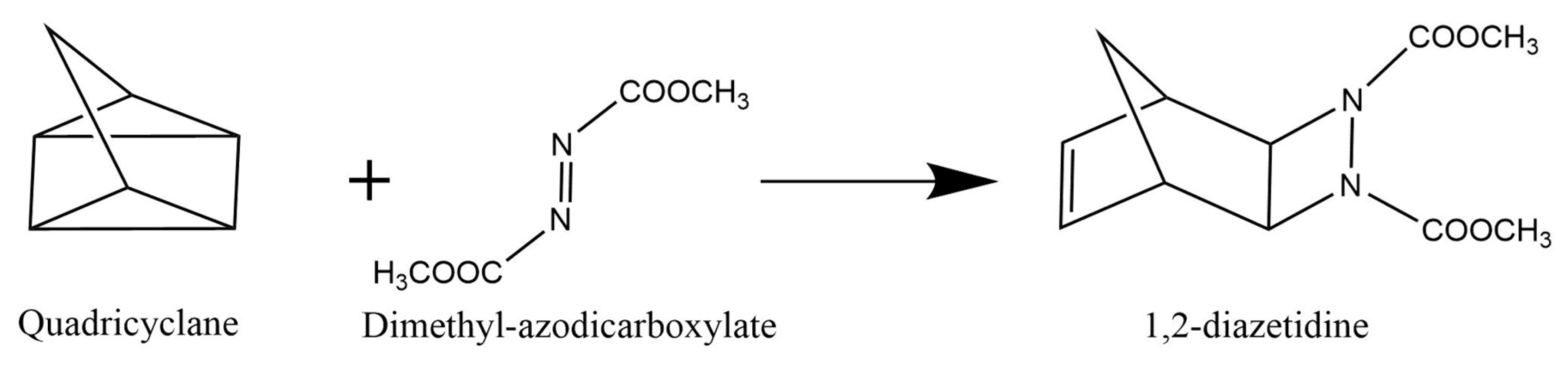
3.1. Organic Reactions ‘on Water’
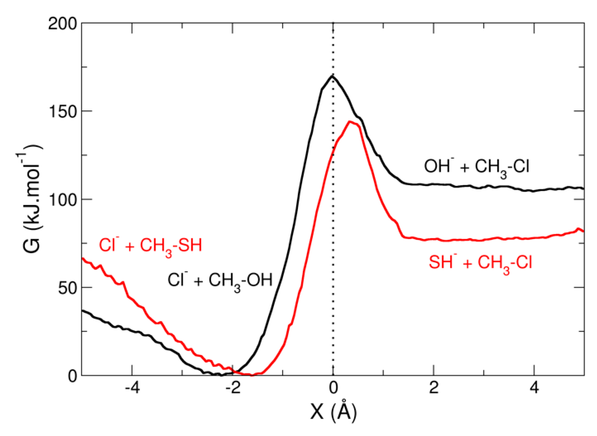
3.2. Umbrella Sampling for a Chemical Reaction
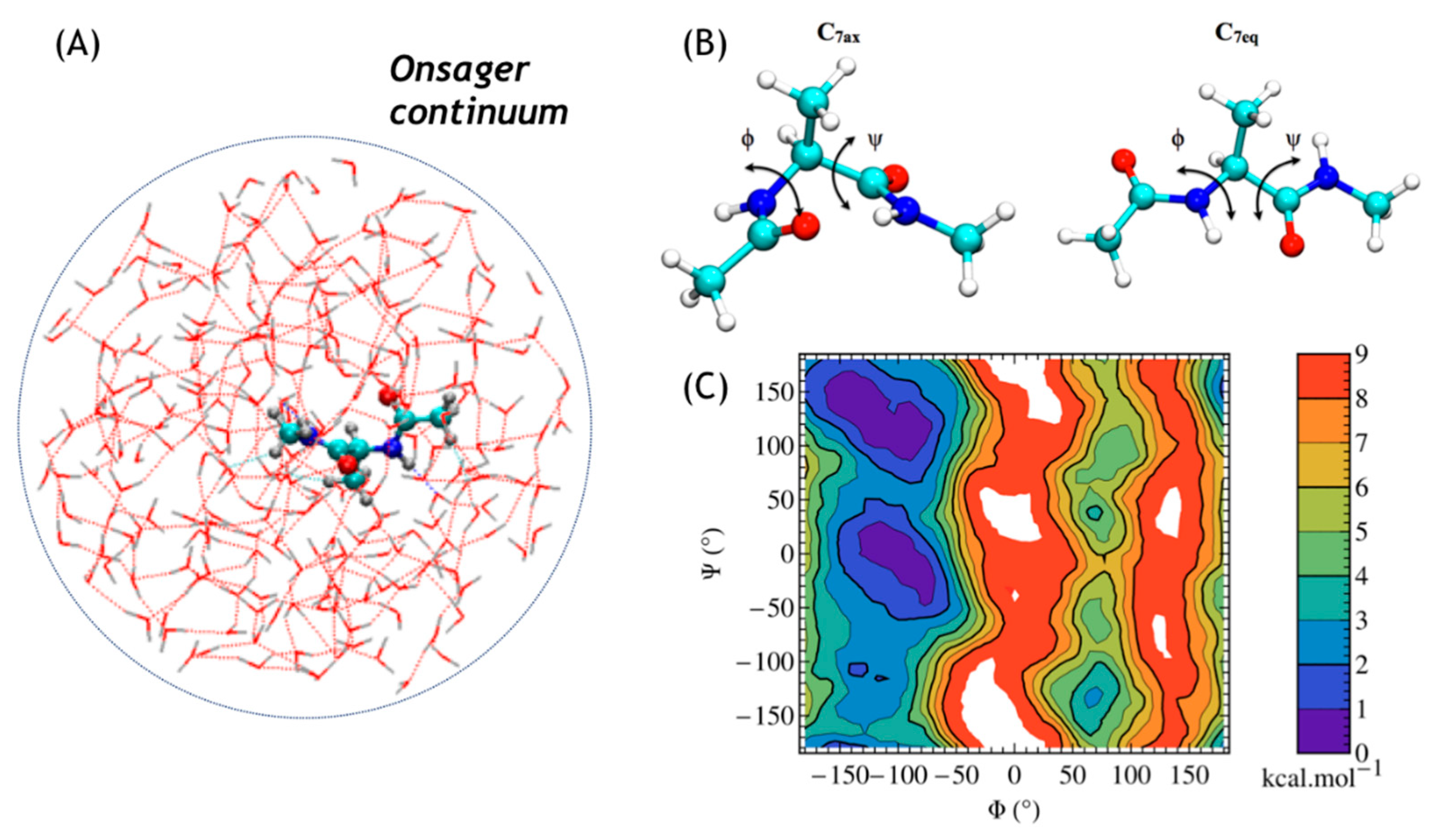
3.3. Two-Dimensional Free Energy Surfaces
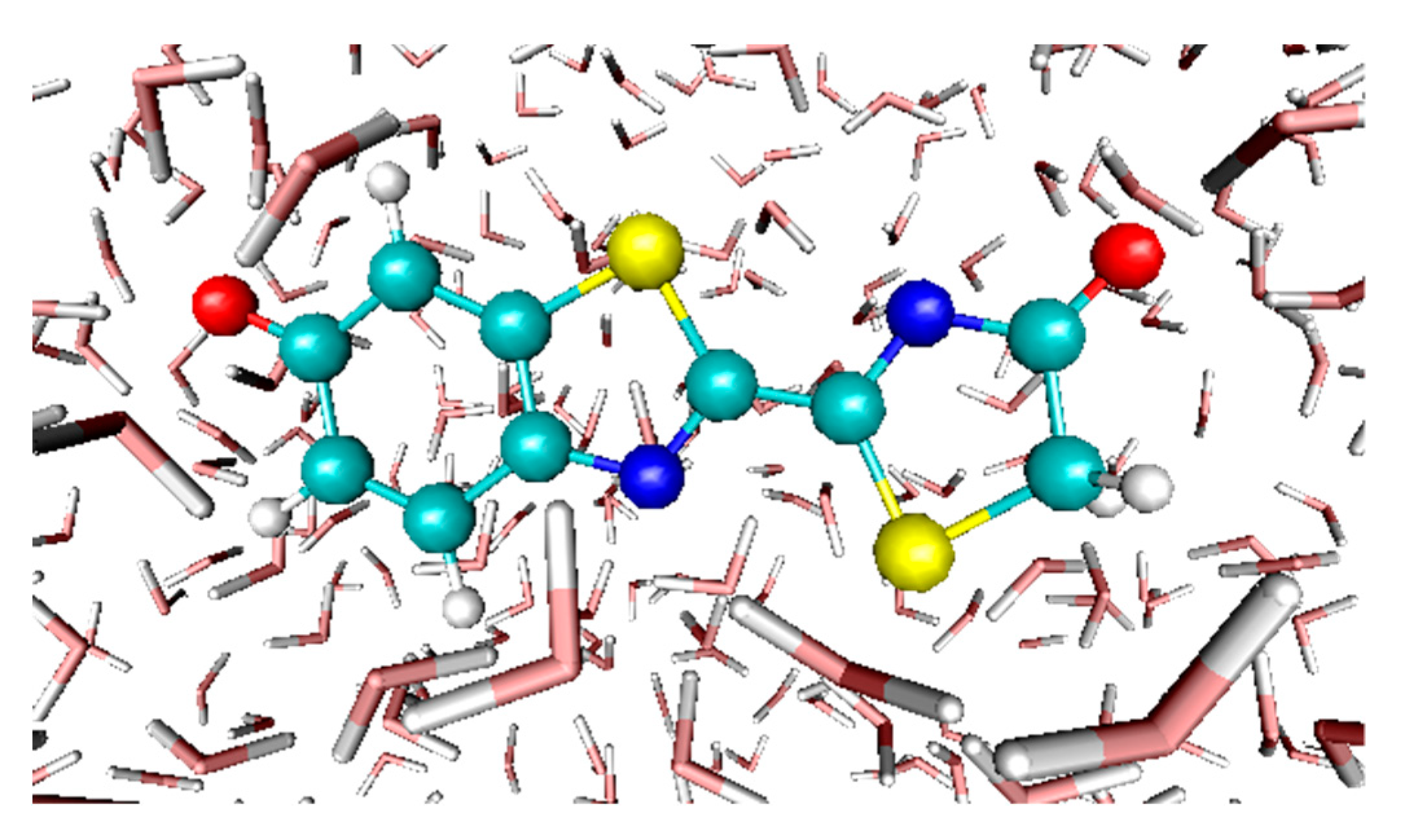
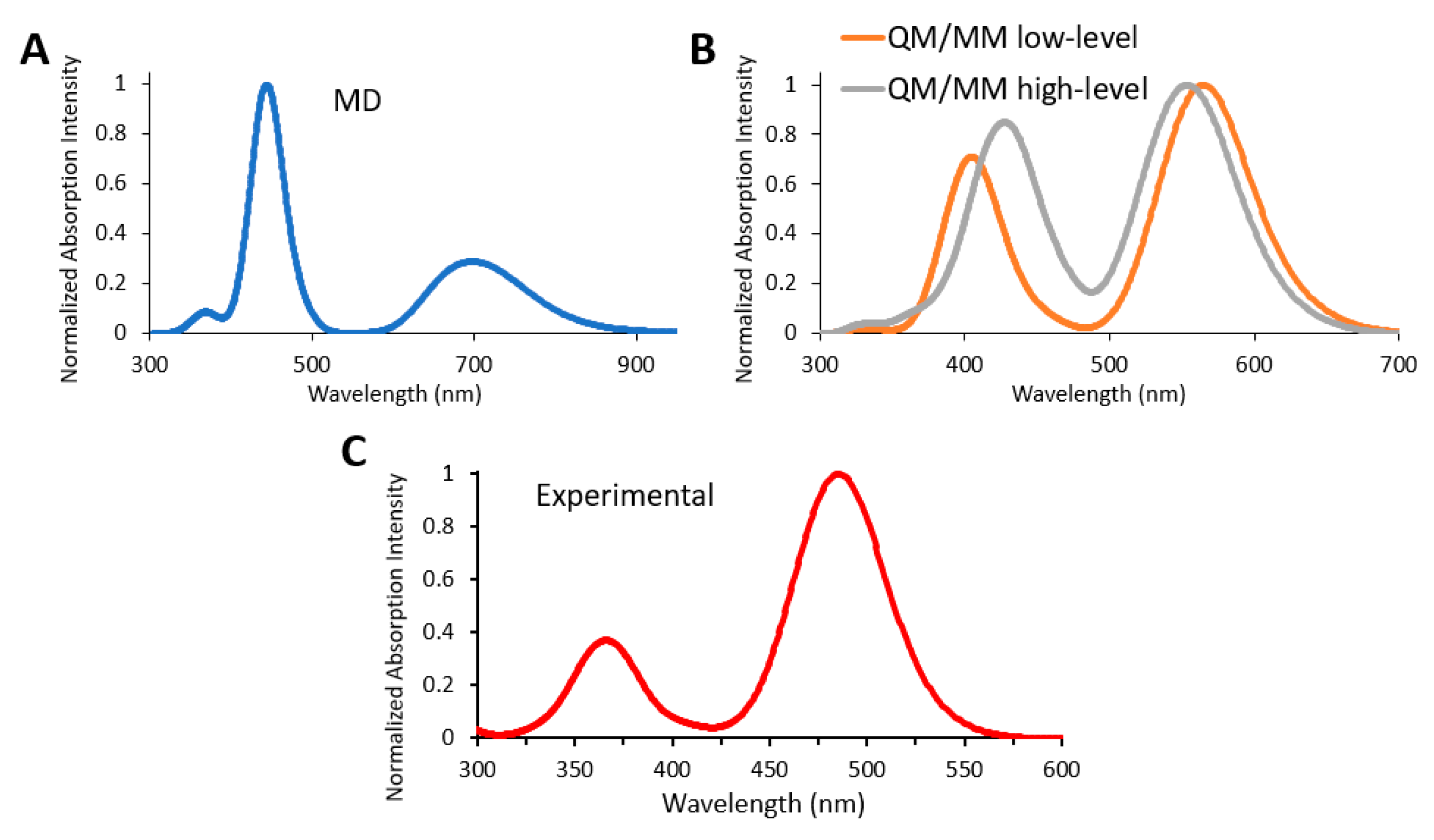
3.4. Absorption Spectra of a Biological Chromophore
3.5. Electron Transfer Free-Energy Profile
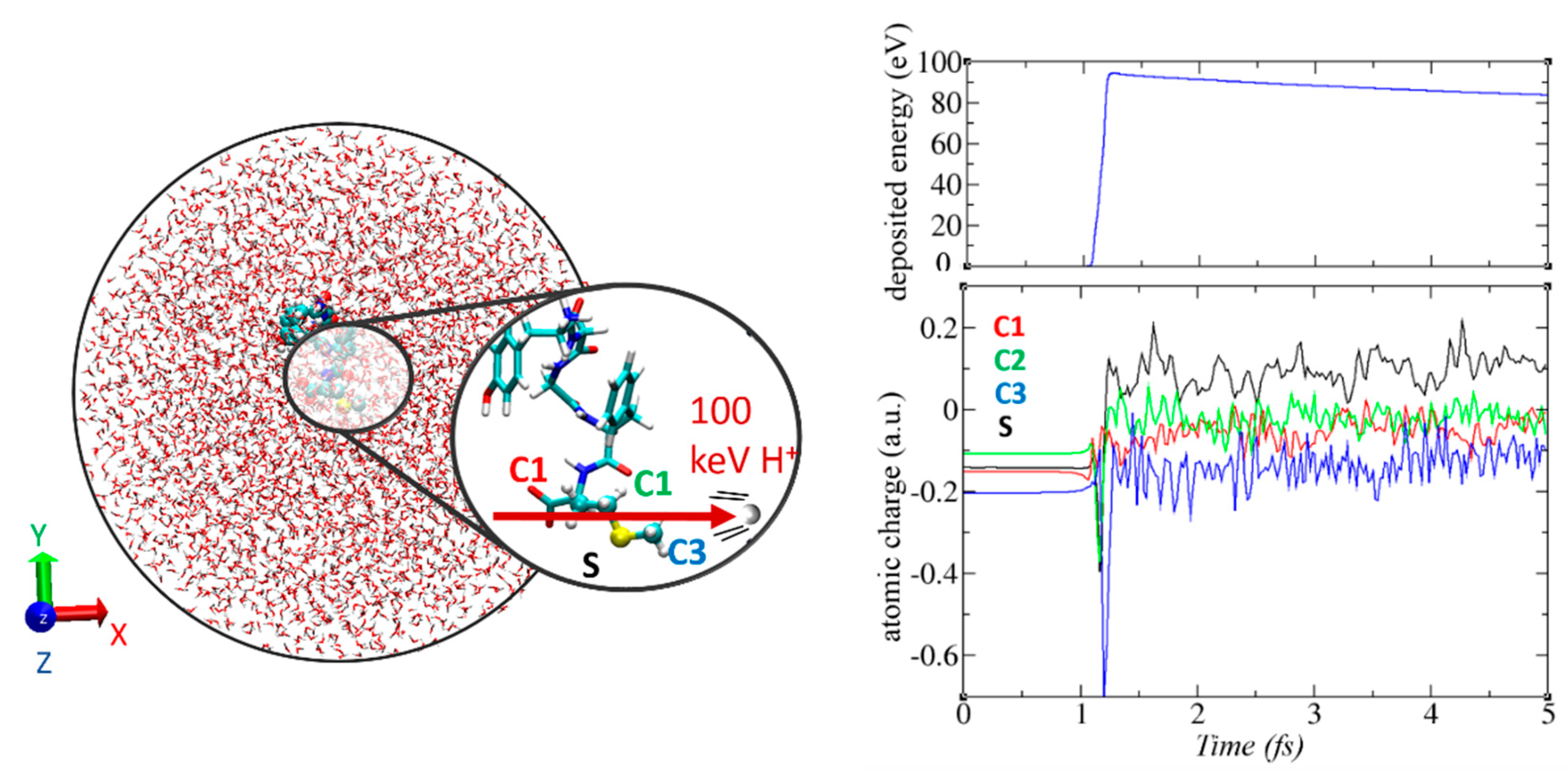
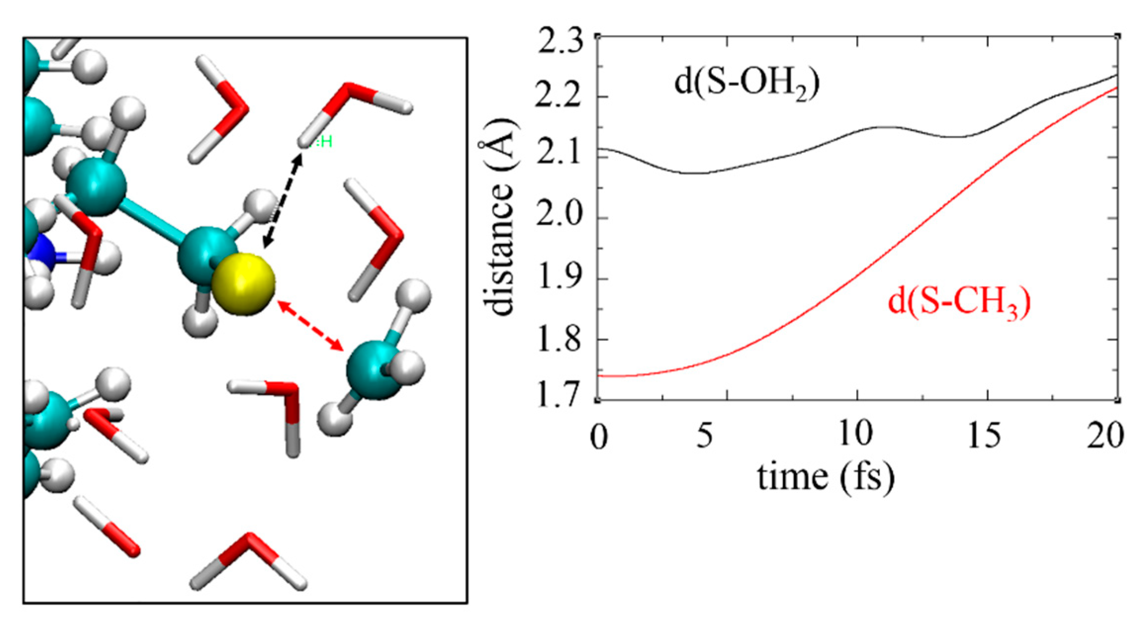
3.6. Non-Adiabatic Chemistry Induced by Ionizing Radiation
4. Conclusions
Author Contributions
Funding
Acknowledgments
Conflicts of Interest
References
- Warshel, A.; Levitt, M. Theoretical studies of enzymic reactions: Dielectric, electrostatic and steric stabilization of the carbonium ion in the reaction of lysozyme. J. Mol. Biol. 1976, 103, 227–249. [Google Scholar] [CrossRef]
- Field, M.J.; Bash, P.A.; Karplus, M. A combined quantum mechanical and molecular mechanical potential for molecular dynamics simulations. J. Comput. Chem. 1990, 11, 700–733. [Google Scholar] [CrossRef]
- Warshel, A.; Karplus, M. Calculation of ground and excited state potential surfaces of conjugated molecules. I. Formulation and parametrization. J. Am. Chem. Soc. 1972, 94, 5612–5625. [Google Scholar] [CrossRef]
- Senn, H.M.; Thiel, W. QM/MM methods for biomolecular systems. Angew. Chem. Int. Ed. 2009, 48, 1198–1229. [Google Scholar]
- Brunk, E.; Rothlisberger, U. Mixed quantum mechanical/molecular mechanical molecular dynamics simulations of biological systems in ground and electronically excited states. Chem. Rev. 2015, 115, 6217–6263. [Google Scholar] [CrossRef] [PubMed]
- Řezáč, J. Cuby: An integrative framework for computational chemistry. J. Comput. Chem. 2016, 37, 1230–1237. [Google Scholar]
- Torras, J.; Roberts, B.P.; Seabra, G.M.; Trickey, S.B. Chapter One—PUPIL: A software integration system for multi-scale qm/mm-md simulations and its application to biomolecular systems. In Advances in Protein Chemistry and Structural Biology; Karabencheva-Christova, T., Ed.; Academic Press: Oxford, UK, 2015; Volume 100, p. 1. [Google Scholar]
- Metz, S.; Kästner, J.; Sokol, A.A.; Keal, T.W.; Sherwood, P. ChemShell—A modular software package for QM/MM simulations. Wiley Interdiscip. Rev. Comput. Mol. Sci. 2014, 4, 101–110. [Google Scholar] [CrossRef]
- Lin, H.; Zhang, Y.; Pezeshki, S.; Wang, B.; Wu, X.-P.; Gagliardi, L.; Truhlar, D. QMMM 2018; University of Minnesota: Minneapolis, MN, USA, 2018. [Google Scholar]
- Kratz, E.G.; Walker, A.R.; Lagardère, L.; Lipparini, F.; Piquemal, J.-P.; Andrés, C.G. LICHEM: A QM/MM program for simulations with multipolar and polarizable force fields. J. Comput. Chem. 2016, 37, 1019–1029. [Google Scholar] [CrossRef]
- Salomon-Ferrer, R.; Case, D.A.; Walker, R.C. An overview of the Amber biomolecular simulation package. Wiley Interdiscip. Rev. Comput. Mol. Sci. 2013, 3, 198–210. [Google Scholar]
- Valiev, M.; Bylaska, E.J.; Govind, N.; Kowalski, K.; Straatsma, T.P.; Van Dam, H.J.J.; Wang, D.; Nieplocha, J.; Apra, E.; Windus, T.L.; et al. NWChem: A comprehensive and scalable open-source solution for large scale molecular simulations. Comput. Phys. Commun. 2010, 181, 1477–1489. [Google Scholar] [CrossRef]
- Shao, Y.; Gan, Z.; Epifanovsky, E.; Gilbert, A.T.B.; Wormit, M.; Kussmann, J.; Lange, A.W.; Behn, A.; Deng, J.; Feng, X.; et al. Advances in molecular quantum chemistry contained in the Q-Chem 4 program package. Mol. Phys. 2015, 113, 184–215. [Google Scholar] [CrossRef]
- Frisch, M.J.; Trucks, G.W.; Schlegel, H.B.; Scuseria, G.E.; Robb, M.A.; Cheeseman, J.R.; Scalmani, G.; Barone, V.; Mennucci, B.; Petersson, G.A.; et al. Gaussian 09; Gaussian, Inc.: Wallingford, CT, USA, 2009. [Google Scholar]
- Köster, A.M.; Geudtner, G.; Alvarez-Ibarra, A.; Calaminici, P.; Casida, M.E.; Carmona-Espindola, J.; Dominguez, V.; Flores-Moreno, R.; Gamboa, G.U.; Goursot, A.; et al. deMon2k Version 5, Mexico City. 2018. Available online: http://demon-software.com/public_html/program.html (accessed on 22 April 2019).
- Kohn, W.; Sham, L.J. Self-consistent equations including exchange and correlation effects. Phys. Rev. 1965, 140, A1133. [Google Scholar] [CrossRef]
- Mintmire, J.W.; Dunlap, B.I. Fitting the Coulomb potential variationally in linear-combination-of-atomic-orbitals density-functional calculations. Phys. Rev. A 1982, 25, 88. [Google Scholar] [CrossRef]
- Gerald, G.; Florian, J.; Köster, A.M.; Alberto, V.; Patrizia, C. Parallelization of the deMon2k code. J. Comput. Chem. 2006, 27, 483–490. [Google Scholar]
- Salahub, D.; Noskov, S.; Lev, B.; Zhang, R.; Ngo, V.; Goursot, A.; Calaminici, P.; Köster, A.; Alvarez-Ibarra, A.; Mejía-Rodríguez, D.; et al. QM/MM Calculations with deMon2k. Molecules 2015, 20, 4780–4812. [Google Scholar] [CrossRef]
- Amara, P.; Field, M.J. Evaluation of an ab initio quantum mechanical/molecular mechanical hybrid-potential link-atom method. Theor. Chem. Acc. 2003, 109, 43–52. [Google Scholar] [CrossRef]
- Gamboa, G.U.; Calaminici, P.; Geudtner, G.; Köster, A.M. How important are temperature effects for cluster polarizabilities? J. Phys. Chem. A 2008, 112, 11969–11971. [Google Scholar] [CrossRef]
- Vásquez-Pérez, J.M.; Martínez, G.U.G.; Köster, A.M.; Calaminici, P. The discovery of unexpected isomers in sodium heptamers by Born–Oppenheimer molecular dynamics. J. Chem. Phys. 2009, 131, 124126. [Google Scholar] [CrossRef] [PubMed]
- Alvarez-Ibarra, A.; Calaminici, P.; Goursot, A.; Gómez-Castro, C.Z.; Grande-Aztatzi, R.; Mineva, T.; Salahub, D.R.; Vásquez-Pérez, J.M.; Vela, A.; Zuniga-Gutierrez, B.; et al. Chapter 7—First Principles Computational Biochemistry with deMon2k A2 - Ul-Haq, Zaheer. In Frontiers in Computational Chemistry; Madura, J.D., Ed.; Bentham Science Publishers: Sharjah, UAE, 2015; p. 281. [Google Scholar]
- Wu, X.; Teuler, J.-M.; Cailliez, F.; Clavaguéra, C.; Salahub, D.R.; de la Lande, A. Simulating electron dynamics in polarizable environments. J. Chem. Theor. Comput. 2017, 13, 3985–4002. [Google Scholar] [CrossRef]
- Wu, X.; Alvarez-Ibarra, A.; Salahub, D.R.; de la Lande, A. Retardation in electron dynamics simulations based on time-dependent density functional theory. Eur. Phys. J. D 2018, 72, 206. [Google Scholar] [CrossRef]
- Tribello, G.A.; Bonomi, M.; Branduardi, D.; Camilloni, C.; Bussi, G. PLUMED 2: New feathers for an old bird. Comput. Phys. Commun. 2014, 185, 604–613. [Google Scholar] [CrossRef]
- Cuny, J.; Korchagina, K.; Menakbi, C.; Mineva, T. Metadynamics combined with auxiliary density functional and density functional tight-binding methods: Alanine dipeptide as a case study. J. Mol. Model. 2017, 23, 72. [Google Scholar] [CrossRef] [PubMed]
- Koster, A.M.; Alvarez-Ibarra, G.G.A.; Calaminici, P.; Casida, M.E.; Carmona-Espindola, J.; Dominguez, V.D.; Flores-Moreno, R.; Gamboa, G.U.; Goursot, A. deMon2k. Available online: http://www.demon-software.com (accessed on 26 April 2019).
- Wang, J.; Wolf, R.M.; Caldwell, J.W.; Kollman, P.A.; Case, D.A. Development and testing of a general amber force field. J. Comput. Chem. 2005, 26, 1157–1174. [Google Scholar] [CrossRef] [PubMed]
- MacKerell, A.D.; Bashford, D.; Bellott, M.; Dunbrack, R.L.; Evanseck, J.D.; Field, M.J.; Fischer, S.; Gao, J.; Guo, H.; Ha, S.; et al. All-atom empirical potential for molecular modeling and dynamics studies of proteins. J. Phys. Chem. B 1998, 102, 3586–3616. [Google Scholar] [CrossRef]
- Foloppe, N.; MacKerell, J. Alexander D. All-atom empirical force field for nucleic acids: I. Parameter optimization based on small molecule and condensed phase macromolecular target data. J. Comput. Chem. 2000, 21, 86–104. [Google Scholar] [CrossRef]
- MacKerell, A.D., Jr.; Banavali, N.K. All-atom empirical force field for nucleic acids: II. Application to molecular dynamics simulations of DNA and RNA in solution. J. Comput. Chem. 2000, 21, 105–120. [Google Scholar] [CrossRef]
- Jorgensen, W.L.; Maxwell, D.S.; Tirado-Rives, J. Development and testing of the opls all-atom force field on conformational energetics and properties of organic liquids. J. Am. Chem. Soc. 1996, 118, 11225–11236. [Google Scholar] [CrossRef]
- Piotr, C.; François-Yves, D.; Yong, D.; Junmei, W. Polarization effects in molecular mechanical force fields. J. Phys. Condens. Matter 2009, 21, 333102. [Google Scholar]
- Caldwell, J.W.; Kollman, P.A. Structure and properties of neat liquids using nonadditive molecular dynamics: Water, methanol, and N-methylacetamide. J. Phys. Chem. 1995, 99, 6208–6219. [Google Scholar] [CrossRef]
- Wang, Z.-X.; Zhang, W.; Wu, C.; Lei, H.; Cieplak, P.; Duan, Y. Strike a balance: Optimization of backbone torsion parameters of AMBER polarizable force field for simulations of proteins and peptides. J. Comput. Chem. 2006, 27, 781–790. [Google Scholar] [CrossRef]
- Thole, B.T. Molecular polarizabilities calculated with a modified dipole interaction. Chem. Phys. 1981, 59, 341–350. [Google Scholar] [CrossRef]
- van Duijnen, P.T.; Swart, M. Molecular and atomic polarizabilities: Thole’s model revisited. J. Phys. Chem. A 1998, 102, 2399. [Google Scholar] [CrossRef]
- Mineva, T.; Russo, N. Solvent effects computed with the Gaussian density functional method. Int. J. Quantum Chem. 1997, 61, 665–671. [Google Scholar] [CrossRef]
- Eurenius, K.P.; Chatfield, D.C.; Brooks, B.R.; Hodoscek, M. Enzyme mechanisms with hybrid quantum and molecular mechanical potentials. I. Theoretical considerations. Int. J. Quantum Chem. 1996, 60, 1189–1200. [Google Scholar] [CrossRef]
- Eichler, U.; Kölmel, C.M.; Sauer, J. Combining ab initio techniques with analytical potential functions for structure predictions of large systems: Method and application to crystalline silica polymorphs. J. Comput. Chem. 1997, 18, 463–477. [Google Scholar] [CrossRef]
- Hohenberg, P.; Kohn, W. Inhomogeneous electron gas. Phys. Rev. 1964, 136, B864. [Google Scholar] [CrossRef]
- Levy, M. Universal variational functionals of electron densities, first-order density matrices, and natural spin-orbitals and solution of the v-representability problem. Proc. Natl. Acad. Soc. USA 1979, 76, 6062–6065. [Google Scholar] [CrossRef]
- Levy, M.; Perdew, J.P. The constrained search formulation of density functional theory. In Density Functional Methods In Physics, 1st ed.; Dreizler, R.M., Providência, J.d., Eds.; Springer US: New York, NY, USA, 1985. [Google Scholar]
- Dunlap, B.I.; Connolly, J.W.D.; Sabin, J.R. On first-row diatomic molecules and local density models. J. Chem. Phys. 1979, 71, 4993–4999. [Google Scholar] [CrossRef]
- Köster, A.M. Hermite Gaussian auxiliary functions for the variational fitting of the Coulomb potential in density functional methods. J. Chem. Phys. 2003, 118, 9943–9951. [Google Scholar]
- Köster, A.M.; Campo, J.M.d.; Janetzko, F.; Zuniga-Gutierrez, B. A MinMax self-consistent-field approach for auxiliary density functional theory. J. Chem. Phys. 2009, 130, 114106. [Google Scholar]
- Alvarez-Ibarra, A.; Köster, A.M. Double asymptotic expansion of three-center electronic repulsion integrals. J. Chem. Phys. 2013, 139, 024102. [Google Scholar] [CrossRef]
- Alvarez-Ibarra, A.; Köster, A.M.; Zhang, R.; Salahub, D.R. Asymptotic expansion for electrostatic embedding integrals in QM/MM calculations. J. Chem. Theor. Comput. 2012, 8, 4232–4238. [Google Scholar] [CrossRef]
- Köster, A.M.; Reveles, J.U.; del Campo, J.M. Calculation of exchange-correlation potentials with auxiliary function densities. J. Chem. Phys. 2004, 121, 3417–3424. [Google Scholar]
- Laikov, D.N. Fast evaluation of density functional exchange-correlation terms using the expansion of the electron density in auxiliary basis sets. Chem. Phys. Lett. 1997, 281, 151–156. [Google Scholar] [CrossRef]
- Mejía-Rodríguez, D.; Köster, A.M. Robust and efficient variational fitting of Fock exchange. J. Chem. Phys. 2014, 141, 124114. [Google Scholar] [CrossRef]
- Mejía-Rodríguez, D.; Huang, X.; del Campo, J.M.; Köster, A.M. Chapter Four—hybrid functionals with variationally fitted exact exchange. In Advances in Quantum Chemistry; Sabin, J.R., Cabrera-Trujillo, R., Eds.; Academic Press: Oxford, UK, 2015; Volume 71, pp. 41–67. [Google Scholar]
- Delesma, F.A.; Geudtner, G.; Mejía-Rodríguez, D.; Calaminici, P.; Köster, A.M. Range-separated hybrid functionals with variational fitted exact exchange. J. Chem. Theor. Comput. 2018, 14, 5608–5616. [Google Scholar] [CrossRef] [PubMed]
- Calaminici, P.; Alvarez-Ibarra, A.; Cruz-Olvera, D.; Domínguez-Soria, V.-D.; Flores-Moreno, R.; Gamboa, G.U.; Geudtner, G.; Goursot, A.; Mejía-Rodríguez, D.; Salahub, D.R.; et al. Auxiliary density functional theory: from molecules to nanostructures. In Handbook of Computational Chemistry; Leszczynski, J., Ed.; Springer: Dordrecht, The Netherlands, 2016; p. 1. [Google Scholar]
- Perdew, J.P.; Burke, K.; Ernzerhof, M. Generalized gradient approximation made simple. Phys. Rev. Lett. 1996, 77, 3865. [Google Scholar] [CrossRef] [PubMed]
- Perdew, J.P.; Ernzerhof, M.; Burke, K. Rationale for mixing exact exchange with density functional approximations. J. Chem. Phys. 1996, 105, 9982–9985. [Google Scholar] [CrossRef]
- Iikura, H.; Tsuneda, T.; Yanai, T.; Hirao, K. A long-range correction scheme for generalized-gradient-approximation exchange functionals. J. Chem. Phys. 2001, 115, 3540–3544. [Google Scholar] [CrossRef]
- Krukau, A.V.; Vydrov, O.A.; Izmaylov, A.F.; Scuseria, G.E. Influence of the exchange screening parameter on the performance of screened hybrid functionals. J. Chem. Phys. 2006, 125, 224106. [Google Scholar] [CrossRef] [PubMed]
- Lange, A.W.; Rohrdanz, M.A.; Herbert, J.M. Charge-transfer excited states in a π-stacked adenine dimer, as predicted using long-range-corrected time-dependent density functional theory. J. Phys. Chem. B 2008, 112, 6304. [Google Scholar] [CrossRef] [PubMed]
- Alvarez-Ibarra, A.; Köster, A.M. A new mixed self-consistent field procedure. Mol. Phys. 2015, 113, 3128–3140. [Google Scholar] [CrossRef]
- Torrie, G.M.; Valleau, J.P. Nonphysical sampling distributions in Monte Carlo free-energy estimation: Umbrella sampling. J. Comput. Phys. 1977, 23, 187–199. [Google Scholar] [CrossRef]
- Kästner, J. Umbrella sampling. Wiley Interdiscip. Rev. Comput. Mol. Sci. 2011, 1, 932–942. [Google Scholar]
- Laio, A.; Gervasio, F.L. Metadynamics: A method to simulate rare events and reconstruct the free energy in biophysics, chemistry and material science. Rep. Prog. Phys. 2008, 71, 126601. [Google Scholar] [CrossRef]
- Barducci, A.; Bonomi, M.; Parrinello, M. Metadynamics. Wiley Interdiscip. Rev. Comput. Mol. Sci. 2011, 1, 826–843. [Google Scholar] [CrossRef]
- Runge, E.; Gross, E.K.U. Density-functional theory for time-dependent systems. Phys. Rev. Lett. 1984, 52, 997. [Google Scholar] [CrossRef]
- Gómez Pueyo, A.; Marques, M.A.L.; Rubio, A.; Castro, A. Propagators for the time-dependent Kohn-Sham equations: Multistep, Runge-Kutta, exponential Runge-Kutta, and commutator free Magnus methods. J. Chem. Theor. Comput. 2018, 14, 3040–3052. [Google Scholar]
- Li, X.; Tully, J.C.; Schlegel, H.B.; Frisch, M.J. Ab initio Ehrenfest dynamics. J. Chem. Phys. 2005, 123, 084106. [Google Scholar] [CrossRef]
- Lopata, K.; Govind, N. Modeling fast electron dynamics with real-time time-dependent density functional theory: Application to small molecules and chromophores. J. Chem. Theor. Comput. 2011, 7, 1344–1355. [Google Scholar] [CrossRef]
- Magnus, W. On the exponential solution of differential equations for a linear operator. Commun. Pure Appl. Math. 1954, 7, 649–673. [Google Scholar] [CrossRef]
- Cheng, C.-L.; Evans, J.S.; Van Voorhis, T. Simulating molecular conductance using real-time density functional theory. Phys. Rev. B 2006, 74, 155112. [Google Scholar] [CrossRef]
- Castro, A.; Marques, M.A.L.; Rubio, A. Propagators for the time-dependent Kohn–Sham equations. J. Chem. Phys. 2004, 121, 3425–3433. [Google Scholar] [CrossRef]
- Gilmore, R. Baker-Campbell-Hausdorff formulas. J. Math. Phys. 1974, 15, 2090–2092. [Google Scholar] [CrossRef]
- Choi, J.; Dongarra, J.J.; Pozo, R.; Walker, D.W. ScaLAPACK: A scalable linear algebra library for distributed memory concurrent computers. In Proceedings of the Fourth Symposium on the Frontiers of Massively Parallel Computation, Washington, DC, USA, 19–21 October 1992; p. 120. [Google Scholar]
- Choi, J.; Demmel, J.; Dhillon, I.; Dongarra, J.; Ostrouchov, S.; Petitet, A.; Stanley, K.; Walker, D.; Whaley, R.C. ScaLAPACK: A portable linear algebra library for distributed memory computers—Design Issues and performance. Comput. Phys. Commun. 1996, 97, 1–15. [Google Scholar] [CrossRef]
- Morzan, U.N.; Ramírez, F.F.; Oviedo, M.B.; Sánchez, C.G.; Scherlis, D.A.; Lebrero, M.C.G. Electron dynamics in complex environments with real-time time dependent density functional theory in a QM-MM framework. J. Chem. Phys. 2014, 140, 164105. [Google Scholar] [CrossRef] [PubMed]
- Donati, G.; Wildman, A.; Caprasecca, S.; Lingerfelt, D.B.; Lipparini, F.; Mennucci, B.; Li, X. Coupling real-time time-dependent density functional theory with polarizable force field. J. Phys. Chem. Lett. 2017, 8, 5283–5289. [Google Scholar] [CrossRef]
- Wildman, A.; Donati, G.; Lipparini, F.; Mennucci, B.; Li, X. Nonequilibrium environment dynamics in a frequency-dependent polarizable embedding model. J. Chem. Theor. Comput. 2019, 15, 43–51. [Google Scholar] [CrossRef]
- Tully, J.C. Mixed quantum-classical dynamics. Faraday Discuss. 1998, 110, 407–419. [Google Scholar] [CrossRef]
- Curchod, B.F.E.; Rothlisberger, U.; Tavernelli, I. Trajectory-based nonadiabatic dynamics with time-dependent density functional theory. ChemPhysChem 2013, 14, 1314–1340. [Google Scholar] [CrossRef]
- Brooks, B.R.; Brooks, C.L., III; Mackerell, A.D., Jr.; Nilsson, L.; Petrella, R.J.; Roux, B.; Won, Y.; Archontis, G.; Bartels, C.; Boresch, S.; et al. CHARMM: The biomolecular simulation program. J. Comput. Chem. 2009, 30, 1545–1614. [Google Scholar] [PubMed]
- Phillips, J.C.; Braun, R.; Wang, W.; Gumbart, J.; Tajkhorshid, E.; Villa, E.; Chipot, C.; Skeel, R.D.; Kalé, L.; Schulten, K. Scalable molecular dynamics with NAMD. J. Comput. Chem. 2005, 26, 1781–1802. [Google Scholar] [CrossRef] [PubMed]
- Ponder, J. Tinker 8—software tools for molecular design. J. Chem. Theory Comput. 2018, 14, 5273–5289. [Google Scholar]
- Lagardere, L.; Jolly, L.-H.; Lipparini, F.; Aviat, F.; Stamm, B.; Jing, Z.F.; Harger, M.; Torabifard, H.; Cisneros, G.A.; Schnieders, M.J.; et al. Tinker-HP: A massively parallel molecular dynamics package for multiscale simulations of large complex systems with advanced point dipole polarizable force fields. Chem. Sci. 2018, 9, 956–972. [Google Scholar] [CrossRef]
- Adamo, C.; Barone, V. Toward reliable density functional methods without adjustable parameters: The PBE0 model. J. Chem. Phys. 1999, 110, 6158. [Google Scholar] [CrossRef]
- Calaminici, P.; Janetzko, F.; Köster, A.M.; Mejia-Olvera, R.; Zuniga-Gutierrez, B. Density functional theory optimized basis sets for gradient corrected functionals: 3d transition metal systems. J. Chem. Phys. 2007, 126, 044108. [Google Scholar] [CrossRef]
- Berweger, C.D.; van Gunsteren, W.F.; Müller-Plathe, F. Force field parametrization by weak coupling. Re-engineering SPC water. Chem. Phys. Lett. 1995, 232, 429–436. [Google Scholar] [CrossRef]
- Reveles, J.U.; Köster, A.M. Geometry optimization in density functional methods. J. Comput. Chem. 2004, 25, 1109–1116. [Google Scholar] [CrossRef] [PubMed]
- Campo, J.M.d.; Köster, A.M. A hierarchical transition state search algorithm. J. Chem. Phys. 2008, 129, 024107. [Google Scholar] [CrossRef]
- Gonzalez, C.; Schlegel, H.B. An improved algorithm for reaction path following. J. Chem. Phys. 1989, 90, 2154. [Google Scholar] [CrossRef]
- Kumar, S.; Rosenberg, J.M.; Bouzida, D.; Swendsen, R.H.; Kollman, P.A. Multidimensional free-energy calculations using the weighted histogram analysis method. J. Comput. Chem. 1995, 16, 1339–1350. [Google Scholar] [CrossRef]
- Kästner, J. Umbrella integration in two or more reaction coordinates. J. Chem. Phys. 2009, 131, 034109. [Google Scholar] [CrossRef] [PubMed]
- Wang, J.; Wang, W.; Kollman, P.A.; Case, D.A. Automatic atom type and bond type perception in molecular mechanical calculations. J. Mol. Gr. Modell. 2006, 25, 247–260. [Google Scholar] [CrossRef] [PubMed]
- Wang, J.; Wolf, R.M.; Caldwell, J.W.; Kollman, P.A.; Case, D.A. Development and testing of a general amber force field. J. Comput. Chem 2004, 25, 1157–1174. [Google Scholar] [CrossRef]
- Jorgensen, W.L.; Chandrasekhar, J.; Madura, J.D.; Impey, R.W.; Klein, M.L. Comparison of simple potential functions for simulating liquid water. J. Chem. Phys. 1983, 79, 926. [Google Scholar] [CrossRef]
- Grossfield, A. WHAM: The Weighted Histogram Analysis Method; 2.0.9; University of Rochester: Rochester, NY, USA, 2013. [Google Scholar]
- Gonzales, J.M.; Cox, R.S.; Brown, S.T.; Allen, W.D.; Schaefer, H.F. Assessment of density functional theory for model SN2 reactions: CH3X + F- (X = F, Cl, CN, OH, SH, NH2, PH2). J. Phys. Chem. A 2001, 105, 11327. [Google Scholar] [CrossRef]
- Doshi, U.; Hamelberg, D. Improved statistical sampling and accuracy with accelerated molecular dynamics on rotatable torsions. J. Chem. Theor. Comput. 2012, 8, 4004–4012. [Google Scholar] [CrossRef]
- Apostolakis, J.; Ferrara, P.; Caflisch, A. Calculation of conformational transitions and barriers in solvated systems: Application to the alanine dipeptide in water. J. Chem. Phys. 1999, 110, 2099. [Google Scholar] [CrossRef]
- García-Iriepa, C.; Gosset, P.; Berraud-Pache, R.; Zemmouche, M.; Taupier, G.; Dorkenoo, K.D.; Didier, P.; Léonard, J.; Ferré, N.; Navizet, I. Simulation and analysis of the spectroscopic properties of oxyluciferin and its analogues in water. J. Chem. Theor. Comput. 2018, 14, 2117–2126. [Google Scholar]
- de la Lande, A.; Cailliez, F.; Salahub, D.R. Electron transfer reactions in enzymes: seven things that might break down in vanilla marcus theory and how to fix them if they do. In Simulating Enzyme Reactivity: Computational Methods in Enzyme Catalysis; Moliner, V., Tunon, I., Eds.; Royal Chemical Society: London, UK, 2017; p. 89. [Google Scholar]
- Warshel, A.; Hwang, J.K. Simulation of the dynamics of electron transfer reactions in polar solvents: Semiclassical trajectories and dispersed polaron approaches. J. Chem. Phys. 1986, 84, 4938. [Google Scholar] [CrossRef]
- King, G.; Warshel, A. Investigation of the free energy functions for electron transfer reactions. J. Chem. Phys. 1990, 93, 8682. [Google Scholar] [CrossRef]
- Warshel, A. Dynamics of reactions in polar solvents. Semiclassical trajectory studies of electron-transfer and proton-transfer reactions. J. Phys. Chem. 1982, 86, 2218–2224. [Google Scholar] [CrossRef]
- Dederichs, P.H.; Blügel, S.; Zeller, R.; Akai, H. Ground states of constrained systems: application to cerium impurities. Phys. Rev. Lett. 1984, 53, 2512. [Google Scholar] [CrossRef]
- Wu, Q.; Van Voorhis, T. Direct optimization method to study constrained systems within density-functional theory. Phys. Rev. A 2005, 72, 024502. [Google Scholar] [CrossRef]
- de la Lande, A.; Salahub, D.R. Derivation of interpretative models for long range electron transfer from constrained density functional theory. J. Mol. Struct. THEOCHEM 2010, 943, 115–120. [Google Scholar] [CrossRef]
- Řezáč, J.; Lévy, B.; Demachy, I.; de la Lande, A. Robust and efficient constrained DFT molecular dynamics approach for biochemical modeling. J. Chem. Theor. Comput. 2012, 8, 418–427. [Google Scholar]
- Blumberger, J. Free energies for biological electron transfer from QM/MM calculation: Method, application and critical assessment. Phys. Chem. Chem. Phys. 2008, 10, 5651–5667. [Google Scholar] [CrossRef]
- Balabin, I.A.; Onuchic, J.N. Dynamically controlled protein tunneling paths in photosynthetic reaction centers. Science 2000, 290, 114–117. [Google Scholar] [CrossRef]
- Mangaud, E.; de la Lande, A.; Meier, C.; Desouter-Lecomte, M. Electron transfer within a reaction path model calibrated by constrained DFT calculations: Application to mixed-valence organic compounds. Phys. Chem. Chem. Phys. 2015, 17, 30889–30903. [Google Scholar] [CrossRef] [PubMed]
- Firmino, T.; Mangaud, E.; Cailliez, F.; Devolder, A.; Mendive-Tapia, D.; Gatti, F.; Meier, C.; Desouter-Lecomte, M.; de la Lande, A. Quantum effects in ultrafast electron transfers within cryptochromes. Phys. Chem. Chem. Phys. 2016, 18, 21442–21457. [Google Scholar] [CrossRef] [PubMed]
- Cailliez, F.; Müller, P.; Firmino, T.; Pernot, P.; de la Lande, A. Energetics of photoinduced charge migration within the tryptophan tetrad of an animal (6–4) photolyase. J. Am. Chem. Soc. 2016, 138, 1904–1915. [Google Scholar] [CrossRef] [PubMed]
- Dunning, T.H. Gaussian basis sets for use in correlated molecular calculations. I. The atoms boron through neon and hydrogen. J. Chem. Phys. 1989, 90, 1007. [Google Scholar] [CrossRef]
- Krause, P.; Sonk, J.A.; Schlegel, H.B. Strong field ionization rates simulated with time-dependent configuration interaction and an absorbing potential. J. Chem. Phys. 2014, 140, 174113. [Google Scholar] [CrossRef] [PubMed]
- Parise, A.; Alvarez-Ibarra, A.; Wu, X.; Zhao, X.; Pilmé, J.; Lande, A.d.l. Quantum chemical topology of the electron localization function in the field of attosecond electron dynamics. J. Phys. Chem. Lett. 2018, 9, 844–850. [Google Scholar] [CrossRef]
- de la Lande, A.; Clavaguéra, C.; Köster, A. On the accuracy of population analyses based on fitted densities. J. Mol. Model. 2017, 23, 99. [Google Scholar] [CrossRef] [PubMed]
- Niklasson, A.M.N.; Steneteg, P.; Odell, A.; Bock, N.; Challacombe, M.; Tymczak, C.J.; Holmström, E.; Zheng, G.; Weber, V. Extended Lagrangian Born–Oppenheimer molecular dynamics with dissipation. J. Chem. Phys. 2009, 130, 214109. [Google Scholar] [CrossRef] [PubMed]
- Huang, J.; MacKerell, A.D., Jr. CHARMM36 all-atom additive protein force field: Validation based on comparison to NMR data. J. Comput. Chem. 2013, 34, 2135–2145. [Google Scholar] [CrossRef] [PubMed]
Sample Availability: Not available. |


| Methods | References |
|---|---|
| Polarizable embedding | [24] |
| Attosecond electron dynamics | [24,25] |
| Ehrenfest non-adiabatic electron-nuclear dynamics | - |
| Link atoms | this work |
| Continuum solvation model for long range interactions | this work |
| Tutorials | this work |
| Geometrical restraints | this work |
| Metadynamics via interface to plumed library [26] | [27], this work |
| Gas Phase (QM) | Liquid Phase (QM/MM) | ||
|---|---|---|---|
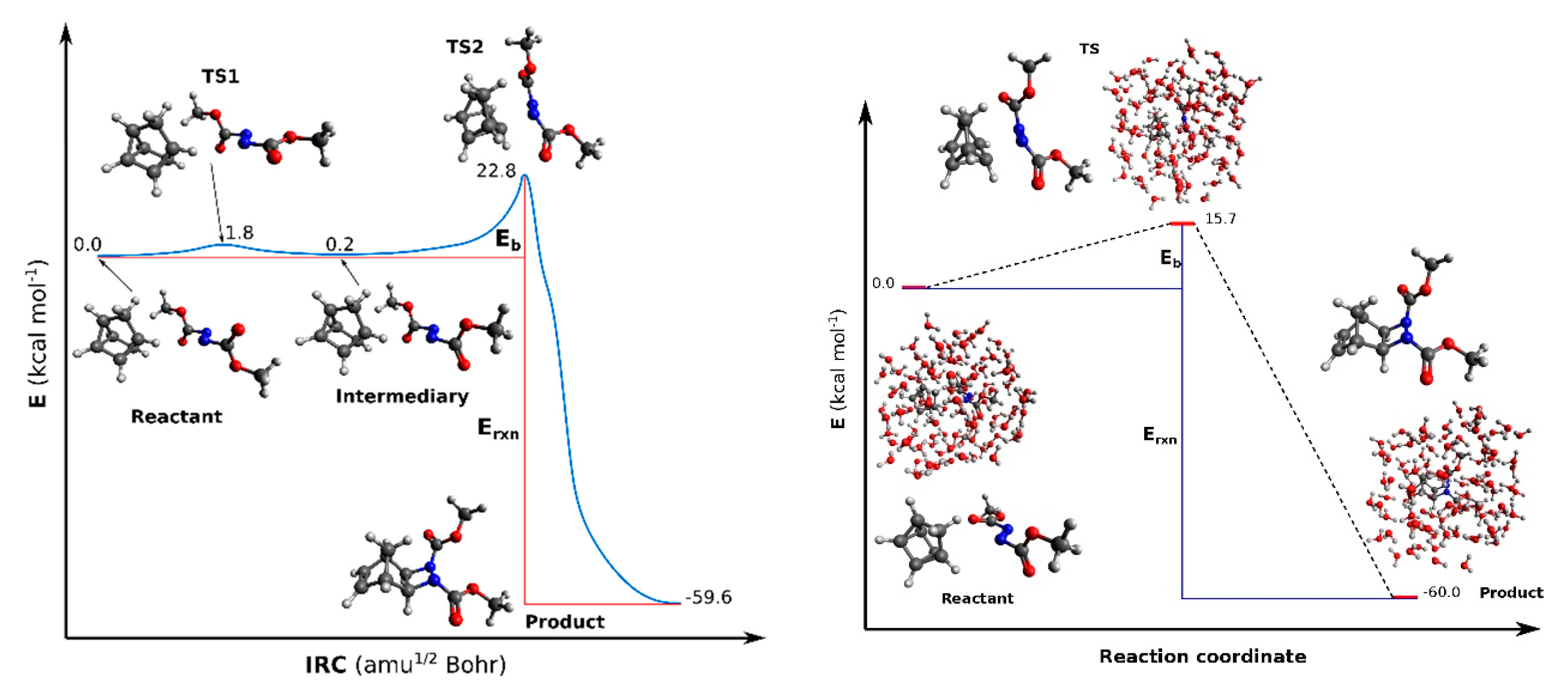
| Eb | Erxn | Eb | Erxn |
| 22.8 | −59.6 | 15.7 | −60.0 |
| Gas Phase (QM) | Liquid Phase (QM/MM) | ||||||
|---|---|---|---|---|---|---|---|
| Reactant | TS1 | Intermediary | TS2 | Product | Reactant | TS | Product |
| 9.2 | 61.0i | 8.3 | 504.4i | 58.8 | 15.2 | 372.8i | 13.9 |
© 2019 by the authors. Licensee MDPI, Basel, Switzerland. This article is an open access article distributed under the terms and conditions of the Creative Commons Attribution (CC BY) license (http://creativecommons.org/licenses/by/4.0/).
Share and Cite
de la Lande, A.; Alvarez-Ibarra, A.; Hasnaoui, K.; Cailliez, F.; Wu, X.; Mineva, T.; Cuny, J.; Calaminici, P.; López-Sosa, L.; Geudtner, G.; et al. Molecular Simulations with in-deMon2k QM/MM, a Tutorial-Review. Molecules 2019, 24, 1653. https://doi.org/10.3390/molecules24091653
de la Lande A, Alvarez-Ibarra A, Hasnaoui K, Cailliez F, Wu X, Mineva T, Cuny J, Calaminici P, López-Sosa L, Geudtner G, et al. Molecular Simulations with in-deMon2k QM/MM, a Tutorial-Review. Molecules. 2019; 24(9):1653. https://doi.org/10.3390/molecules24091653
Chicago/Turabian Stylede la Lande, Aurélien, Aurelio Alvarez-Ibarra, Karim Hasnaoui, Fabien Cailliez, Xiaojing Wu, Tzonka Mineva, Jérôme Cuny, Patrizia Calaminici, Luis López-Sosa, Gerald Geudtner, and et al. 2019. "Molecular Simulations with in-deMon2k QM/MM, a Tutorial-Review" Molecules 24, no. 9: 1653. https://doi.org/10.3390/molecules24091653