Article

Crystal Chemistry of Sulfates from the Apuan Alps (Tuscany, Italy). V. Scordariite, K8(Fe3+0.670.33)[Fe3+3O(SO4)6(H2O)3]2(H2O)11: A New Metavoltine-Related Mineral

1
Dipartimento di Scienze della Terra, Università di Pisa, Via Santa Maria 53, I-56126 Pisa, Italy
2
Dipartimento di Scienze della Terra, Università degli Studi di Firenze, Via G. La Pira 4, I-50121 Firenze, Italy
3
Department of Geosciences, Swedish Museum of Natural History, Box 50007, SE-10405 Stockholm, Sweden
*
Author to whom correspondence should be addressed.
Minerals 2019, 9(11), 702; https://doi.org/10.3390/min9110702
Submission received: 30 October 2019 / Revised: 8 November 2019 / Accepted: 11 November 2019 / Published: 13 November 2019
(This article belongs to the Collection New Minerals)

Abstract

:
The new mineral species scordariite, K8(Fe3+0.670.33)[Fe3+3O(SO4)6(H2O)3]2(H2O)11, was discovered in the Monte Arsiccio mine, Apuan Alps, Tuscany, Italy. It occurs as pseudo-hexagonal tabular crystals, yellowish to brownish in color, up to 0.5 mm in size. Cleavage is perfect on {0001}. It is associated with giacovazzoite, krausite, gypsum, jarosite, alum-(K), and magnanelliite. Electron microprobe analyses give (wt %): SO3 47.31, Al2O3 0.66, Fe2O3 24.68, FeO 0.69, Na2O 0.52, K2O 17.36, H2Ocalc 15.06, total 106.28. The partitioning of Fe between Fe2+ and Fe3+ was based on Mössbauer spectroscopy. On the basis of 67 O atoms per formula unit, the empirical chemical formula is (K7.50Na0.34)Σ7.84(Fe3+6.29Al0.26Fe2+0.20)Σ6.75S12.02O50·17H2O. The ideal end-member formula can be written as K8(Fe3+0.670.33)[Fe3+3O(SO4)6(H2O)3]2(H2O)11. Scordariite is trigonal, space group R-3, with (hexagonal setting) a = 9.7583(12), c = 53.687(7) Å, V = 4427.4(12) Å3, Z = 3. The main diffraction lines of the observed X-ray powder pattern are [d(in Å), estimated visual intensity]: 8.3, strong; 6.6, medium; 3.777, medium; 3.299, medium; 3.189, medium; 2.884, strong. The crystal structure of scordariite has been refined using X-ray single-crystal data to a final R1 = 0.057 on the basis of 1980 reflections with Fo > 4σ(Fo) and 165 refined parameters. It can be described as a layered structure formed by three kinds of layers. As with other metavoltine-related minerals, scordariite is characterized by the occurrence of the [Fe3+3O(SO4)6(H2O)3]5− heteropolyhedral cluster.

1. Introduction

In the last decade, the Monte Arsiccio mine has been studied for its interesting sulfosalt assemblages (e.g., Biagioni et al. [1]) and the occurrence of some very peculiar oxides (e.g., mannardite [2], mapiquiroite [3]). More recently, sulfate assemblages deriving from the weathering of pyrite ores have been investigated, leading to the description of three new mineral species: giacovazzoite [4], magnanelliite [5], and scordariite. All these new species are K–Fe3+ sulfates, likely deriving from the interaction between acidic solutions and K-bearing rocks.
Scordariite and giacovazzoite were found to be closely associated and were initially visually identified on the basis of their distinct morphology and color. Further preliminary investigations through energy-dispersive X-ray spectrometry and X-ray powder diffraction confirmed the distinction between monoclinic giacovazzoite, the natural analogue of β-Maus’ salt [4], and the new mineral scordariite. The name honors Fernando Scordari (b. 1944), a full professor of Mineralogy at the University of Bari since 1986 up until his retirement. He was the president of the Società Italiana di Mineralogia e Petrologia (SIMP) in 1998–2000 and vice-president (along with Thomas Armbruster) of the European Mineralogical Union in 2000–2004. Fernando Scordari is the author of more than 150 papers and three textbooks about crystallography and mass spectrometry. His scientific activity was devoted to the crystal chemistry of minerals and inorganic compounds, with a particular focus on silicates and sulfates. Among the latter, Fernando Scordari gave an important contribution to the crystal chemistry of metavoltine and its related compounds (e.g., Scordari et al. [6]). The mineral and its name have been approved by the IMA-CNMNC (2019-010). The holotype specimen of scordariite is deposited in the mineralogical collection of the Museo di Storia Naturale, Università di Pisa, Via Roma 79, Calci (Pisa), Italy, under catalog number 19893.
This paper presents the definition, occurrence, and crystal structure of the new mineral species scordariite.

2. Occurrence and Physical Properties

The Monte Arsiccio mine (latitude 43°58′ N, longitude 10°17′ E) exploited a pyrite + baryte + iron oxide (magnetite, hematite, “limonite”) ore deposit located in the southern Apuan Alps, northern Tuscany, Italy [7]. The main orebodies are hosted within a Paleozoic metavolcanic–metasedimentary sequence, locally tourmalinized, and close to being in contact with the overlying Triassic metadolostone (“Grezzoni” Formation), belonging to the Apuane Unit. This unit was metamorphosed up to greenschist facies conditions, with T and P conditions between 350–450 °C and 0.3–0.4 GPa (Molli et al. [8] and references therein).
The sulfate assemblage where scordariite was collected occurs in an old stope of the mine where microcrystalline pyrite is exposed and deeply altered. This ongoing oxidation process has given rise to a large suite of secondary phases (Table 1), in some cases occurring as well-crystallized specimens. It is worth noting to stress the occurrence of several K–Fe3+ sulfates. Indeed, among the currently known minerals belonging to the system K2O–Fe2O3–H2O, all occur at the Monte Arsiccio mine, the only exception being represented by yavapaiite, KFe3+(SO4)2, not yet found at this locality. Moreover, three sulfate minerals belonging to this chemical system have their type-locality here: giacovazzoite, magnanelliite, and scordariite.

2.1. Physical Properties

Scordariite forms pseudo-hexagonal {0001} tabular crystals up to 0.5 mm in size (Figure 1). The color varies with thickness, from yellowish to brownish, and the streak is yellowish. It is transparent, vitreous, and displays no fluorescence. Hardness was not measured but it should be close to 2–2½, in agreement with metavoltine [9]. Scordariite is brittle, with a perfect {0001} cleavage, and the fracture is irregular. Density, calculated based on the empirical formula and the unit-cell volume refined from single-crystal X-ray diffraction, is 2.432 g/cm3. It is easily soluble in H2O at room T.
Scordariite is distinctly pleochroic, from pale yellow to yellow. It is uniaxial (–). The mean refractive index, calculated according to the Gladstone-Dale relationship [10,11], is 1.573.
In the studied specimen, scordariite is associated with giacovazzoite and alum-(K). Other minerals observed in association with scordariite are krausite, gypsum, jarosite, and magnanelliite.

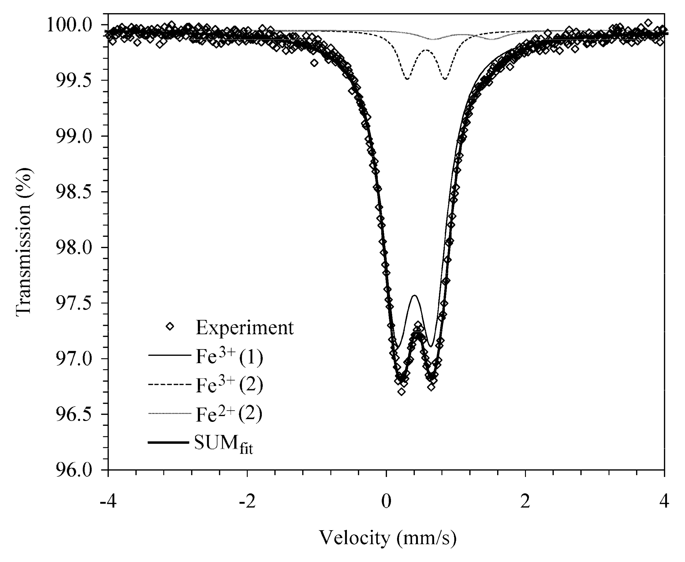
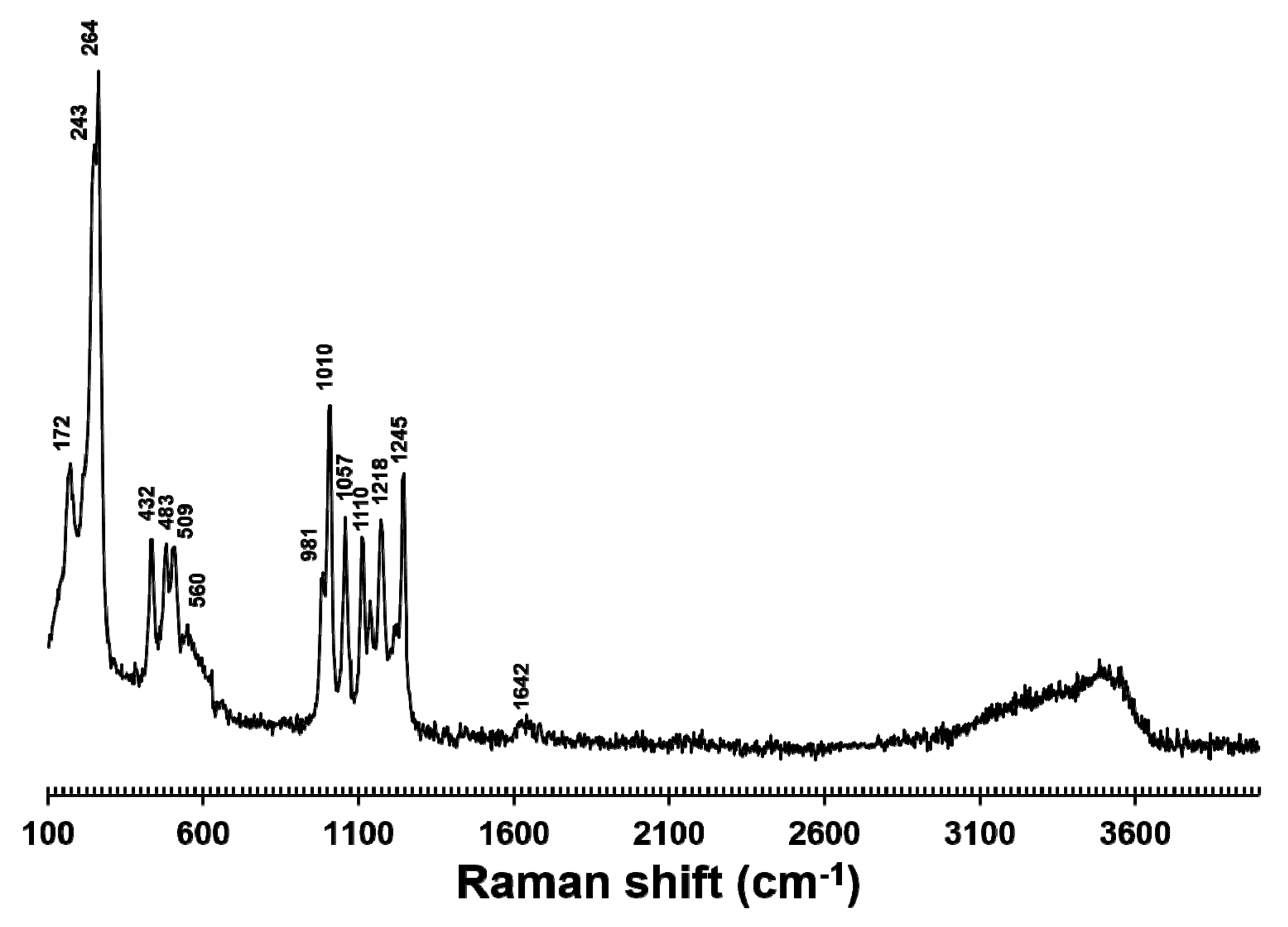
2.2. Chemical and Spectroscopic Data

A preliminary chemical analysis using a FEI Quanta 450 ESEM FEG (FEI Company, Hillsboro, OR, USA) equipped with a QUANTAX Xflash detector 6|10 (EDS mode) (Bruker, Billerica, MA, USA) did not indicate the presence of elements (Z > 9) other than K, Fe, S, and minor Na and Al.
Quantitative chemical data were collected on one polished crystal using a JEOL JXA 8200 electron microprobe (JEOL, Tokyo, Japan) operating in WDS mode at 8 kV and 20 nA, with the beam defocused to 15 μm in diameter in order to limit the sample damage. Analyses were performed under unfavorable conditions, because scordariite slightly decomposed under the electron beam. The relatively high analytical totals obtained after the addition of the calculated H2O content (on the basis of structural data—see below) were likely due to the partial dehydration of the sample under high vacuum during carbon coating or during electron microprobe analysis. Dehydration was manifested via fractures in the sample surface. The following standards (element, emission line) were used: synthetic MgSO4 (SKα), albite (AlKα, NaKα), hematite (FeKα), and sanidine (KKα). Chemical data are given in Table 2.
The empirical formula of scordariite, calculated on the basis of 67 O atoms per formula unit (apfu), was (K7.50Na0.34)Σ7.84(Fe3+6.29Al0.26Fe2+0.20)Σ6.75S12.02O50·17H2O. Taking into account the structural data, as well as the Mössbauer spectroscopic data (see below), the following formula could be proposed (K7.50Na0.34)Σ7.84(Fe3+0.41Fe2+0.20Al0.13)Σ0.74[(Fe3+2.94Al0.06)Σ3.00O(SO4)6(H2O)3]2(H2O)11, with rounding errors. The end-member formula of scordariite could be written as K8(Fe3+0.670.33)[Fe3+3O(SO4)6(H2O)3]2(H2O)11, corresponding to (in wt %): SO3 44.14, Fe2O3 24.47, K2O 17.31, H2O 14.08, sum 100.00.
The 57Fe Mössbauer spectrum of scordariite (Figure 2) was acquired at room T in transmission mode using a 57Co (in Rh matrix) point source with nominal activity of 0.40 GBq (Natural History Museum, Stockholm, Sweden) over the velocity range ±4 mm/s and was calibrated against α-Fe foil. Data were collected in 1024 channels with a constant acceleration system equipped with a proportional gas-filled counter on an absorber consisting of less than 1 mg mineral powder between mylar windows over 84 h. The spectrum was fitted using the program MossA [12] by applying a fitting model with three quadrupole doublets. The resulting fit (Figure 2) is comprised of one intense quadrupole doublet with a small CS-value of 0.40 mm/s and a low-intensity doublet with a CS-value of 0.57 mm/s. Both doublets show CS-values typical for ferric iron at six-coordinated sites in oxygen-based structures. The higher CS-value of the low-intensity Fe3+-doublet suggests that this Fe occurred in a site with longer Fe–O bonds. A further doublet with very low intensity (3% of the total iron content of the sample) and a higher CS-value of 1.04 mm/s is assigned to ferrous iron in an octahedral coordination.
The Mössbauer spectrum of scordariite (Figure 2) indicates an atomic ratio Fe2+/Fetot of 0.03; consequently, 97% of total iron is represented by Fe3+, partitioned between Fe(1) (88% of total iron) and Fe(2) (9% of total iron).
Micro-Raman spectra were obtained on an unpolished sample of scordariite with a nearly back-scattered geometry with a Horiba Jobin-Yvon XploRA Plus apparatus (Horiba France SAS, Longjumeau Cedex, France), equipped with a motorized x-y stage and an Olympus BX41 microscope (SPOT Imaging, Sterling Heights, MI, USA) with a 10× objective. The 532 nm line of a solid-state laser was used. The minimum lateral and depth resolution was set to a few μm. The system was calibrated using the 520.6 cm−1 Raman band of silicon before each experimental session. Spectra were collected through three acquisitions with single counting times of 100 s, with the laser power filtered at 25% (i.e., 6.25 mW). No thermal damage was observed. Backscattered radiation was analyzed with a 1200 mm−1 grating monochromator. Figure 3 shows the Raman spectrum of scordariite. Between 400 and 1200 cm−1, Raman bands related to SO4 modes occur. The strongest bands in the range 950–1250 cm−1 are related to the symmetrical (at 981, 1010, and 1057 cm−1) and the antisymmetrical stretching (at 1110, 1144, 1171, 1218, and 1245 cm−1) modes. Bending modes occur at 432 and 483 cm−1 (ν2 modes), as well as at 509 and 560 cm−1 (ν4 modes). Lattice vibrations and Fe–O modes are present in the range 100–300 cm−1 (172, 243, and 264 cm−1). The occurrence of H2O groups is confirmed by the presence of broad bands between 3000 and 3600 cm−1, interpreted as being due to the O–H stretching modes. Finally, a weak band at 1642 cm−1 can be attributed to the bending of O–H–O bonds.

2.3. X-ray Crystallography

X-ray powder diffraction data of scordariite (Table 3) were collected using a 114.6 mm Gandolfi camera and Ni-filtered CuKα radiation. Unit-cell parameters were refined using the software CELREF [13] using a hexagonal setting and the space group R-3: a = 9.762(6), c = 53.5030(10) Å, V = 4415(3) Å3.
Intensity data were collected using a Bruker AXS Smart Breeze diffractometer (Bruker AXS Inc., Madison, WI, USA) equipped with a Photon II air-cooled CCD detector (Bruker, Billerica, MA, USA) and graphite-monochromatized MoKα radiation. The detector to crystal distance was 50 mm. Data were collected using ω and φ scan modes, in 0.1° slices, with an exposure time of 20 s per frame. Data were corrected for the Lorentz, polarization, absorption, and background effects using the package of software Apex3 [14]. The statistical test on the distribution of |E| values (|E2 – 1| = 0.819) and the examination of the reflection conditions suggested the space group R-3 or R3. The crystal structure was solved in R-3 using Shelxs-97 and it was refined using Shelxl-2018 [15]. Eight cation and twelve anion sites were located. Among the cation sites, four were K-sites [K(1)–K(4)], two sites [Fe(1) and Fe(2)] hosted Fe, and S occurred at two S sites, namely S(1) and S(2). Scattering curves for neutral atoms were taken from the International Tables for Crystallography [16]. The refinement of the initial structural model converged to R1 = 0.35, lowered to R1 = 0.10 assuming the occurrence of twinning according to a two-fold axis along [0001]. The ratio between the two twinned components was 0.79(1):0.21. The sites K(4) and Fe(2) were found to be partially occupied. In detail, K(4) showed short K(4)–K(4) distances (3.34 Å) and the site occupancy factor (s.o.f.) pointed to K0.52(1), which was then fixed to K0.50 in order to avoid short K–K contacts. The examination of the difference Fourier maps in the latest stages of the refinement, however, revealed a maximum close to K(4) that could be interpreted as a split position, likely hosting the oxygen atom of an H2O group, labelled as Ow(1). The s.o.f. at the Fe(2) site was refined to Fe0.66(1). The introduction of anisotropic displacement parameters for cations only lowered the R1 factor to 0.08, which was further improved through an anisotropic description of the displacement parameters of anions (R1 = 0.06). Among the O sites, Ow(4) had high displacement parameters, suggesting a possible splitting of this position. However, a satisfying split model was not obtained. In addition, a maximum in the difference-Fourier maps suggested the occurrence of a partially filled Na site, mutually exclusive with K(4). Consequently, the s.o.f. at K(4) and Na(4) were fixed in agreement with electron microprobe data, assuming (K7.50Na0.50) and hypothesizing that the small Na deficit (0.34 Na apfu according to chemical analysis) could be due to Na volatilization under the electron beam. Finally, the position of H atoms bonded to oxygen atoms hosted at the Ow(2) and Ow(3) sites were located and soft restraints were added in order to avoid too short O–H distances. The crystal structure refinement converged to R1 = 0.0571 for 1980 reflections with Fo > 4σ(Fo) (0.0624 for all 2156 data) and 165 refined parameters.
Details of the data collection and structure refinement are given in Table 4. Atomic coordinates, displacement parameters, and bond distances are reported in Table 5. The CIF of scordariite is available as Supplementary Materials linked to this article.

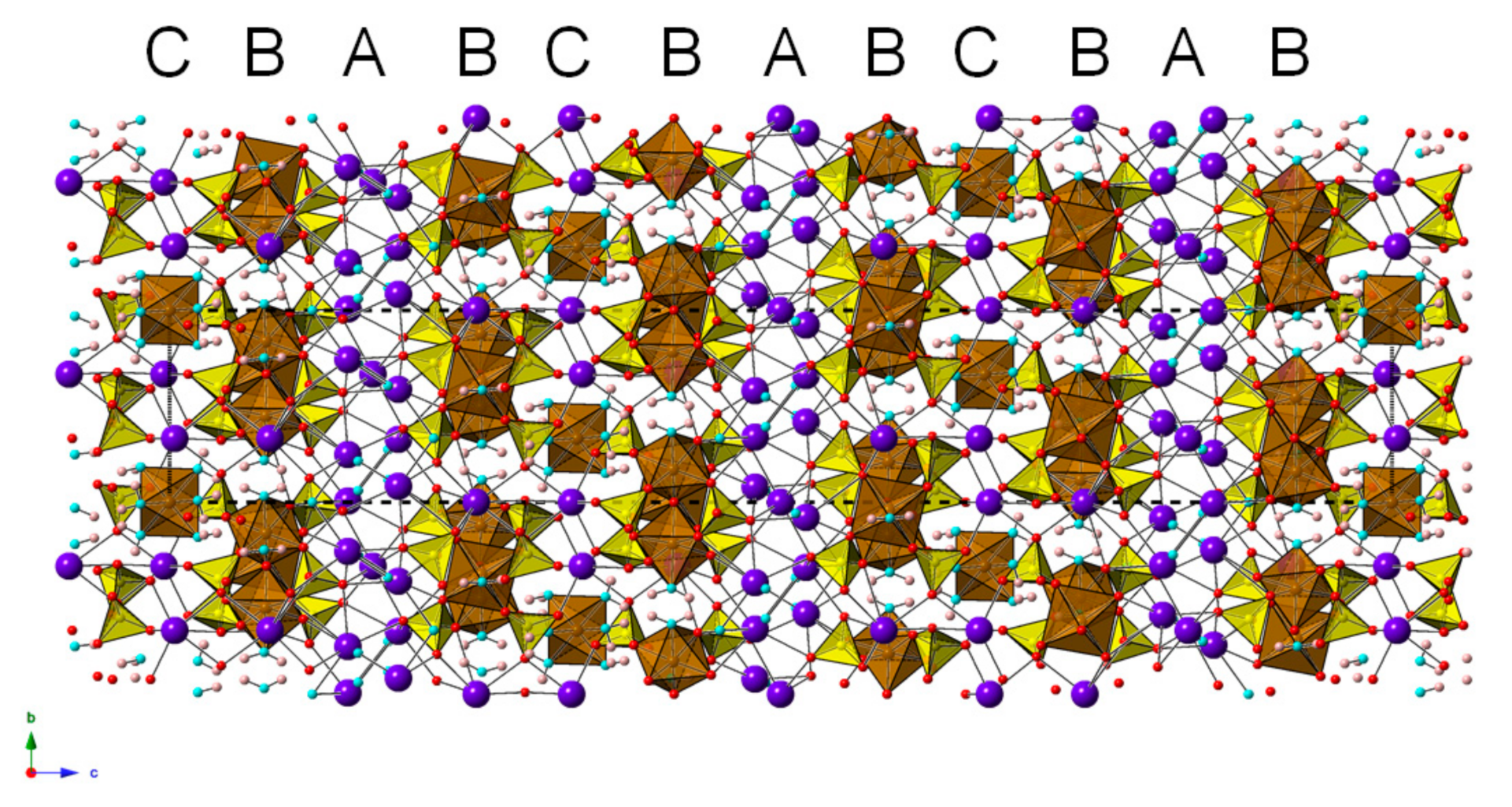
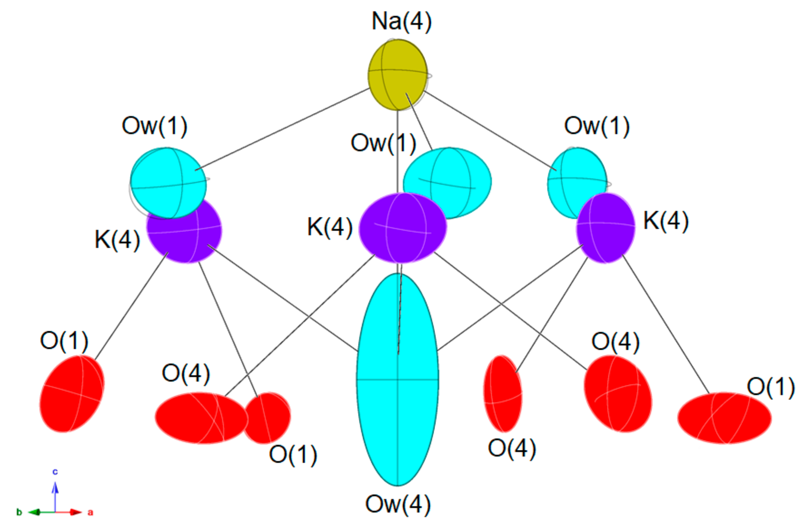
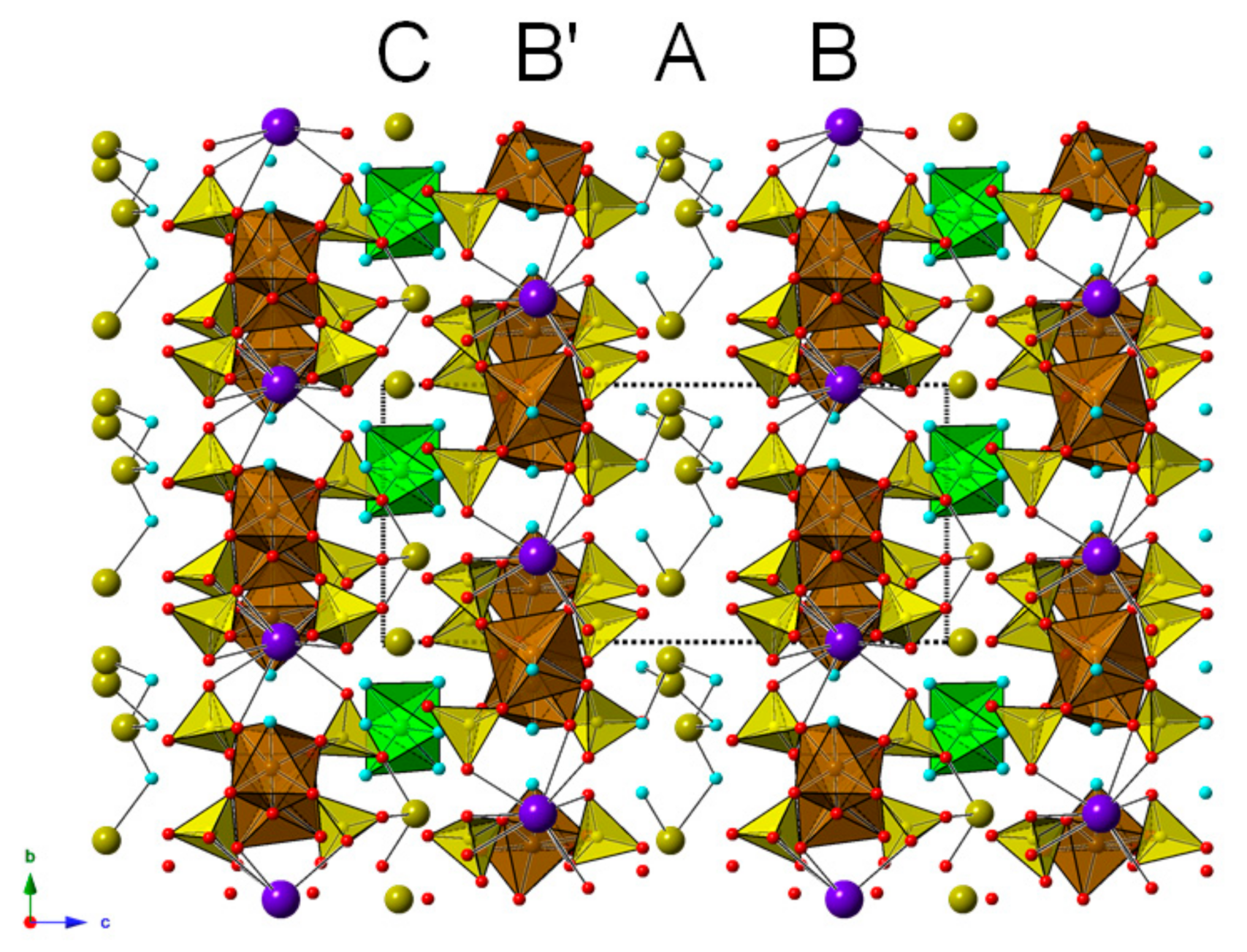
3. Crystal Structure Description

Nine independent cation sites (some of them only partially occupied) and thirteen anion positions (one of them split into three sub-positions) occur in the crystal structure of scordariite. Table 6 reports selected bond distances, whereas bond-valence sums (BVS), calculated according to the bond parameters of Brese and O’Keeffe [18], are shown in Table 7.
Potassium is hosted at four distinct sites, i.e., K(1)–K(4). K(1) and K(2) have a distorted octahedral coordination, with average bond distances of 2.796 and 2.744 Å, respectively. Their BVS are 1.02 and 1.17 valence units (v.u.), respectively. K(3) has a distorted tricapped trigonal prismatic coordination, with bond distances ranging from 2.824 to 3.073 Å, with an average <K–O> distance of 2.963 Å. Its BVS is 0.99 v.u. The site K(4) is only partially occupied. It is seven-fold coordinated, being coordinated by five O2− anions and two H2O groups hosted at Ow(1) and Ow(4). The average <K–O> distance is 2.942 Å, with values ranging between 2.751 and 3.363 Å; assuming its full occupancy, the corresponding BVS is 0.92 v.u. The partially occupied Na(4) site is at 2.67 Å from Ow(1); in addition, it is bonded to Ow(4), although the observed distance is too long (i.e., 3.10 Å). It is worth noting that the high displacement parameter shown by Ow(4) suggests that when the Na(4) site is occupied by Na+, the H2O group could be displaced toward this site. Na(4) is located in a position similar to the Na(4) site of metavoltine [19]; however, in this latter mineral, Na is six-fold coordinated by H2O groups, with bond distances ranging between 2.39 and 2.49 Å. It is likely that the low s.o.f. of Na(4) in scordariite did not allow for an accurate description of its coordination environment.
Ferric iron is hosted at Fe(1), with bond distances ranging between 1.922 and 2.110 Å, the longest distance being formed with the H2O group hosted at Ow(2). Average bond distance is 2.010 Å, compared with 1.985 and 2.00 Å observed in metavoltine [19]. Its BVS is 3.08 v.u. Three symmetry-related Fe(1) sites form a cluster sharing the oxygen atom hosted at O(9). This trimer is bonded through corner-sharing with six SO4 groups, represented by two different sites, S(1) and S(2). The S–O distances range between 1.439 and 1.497 Å, with average bond distances of 1.469 and 1.470 Å at the S(1) and S(2) sites, respectively. BVS at the S(1) and S(2) are 6.09 and 6.07 v.u., respectively.
Ferric iron, along with minor Fe2+, is also hosted at the partially occupied Fe(2) site. The refined site scattering gives 17.4 electrons per formula unit (epfu). The Mössbauer spectroscopy indicates that 88% Fe is partitioned at Fe(1), whereas 12% of the total Fe occurs at Fe(2). In addition, 3% of the total Fe is represented by Fe2+. Taking into account such results, assuming that minor Al (0.26 apfu) is completely partitioned at Fe(1), the site occupancy at Fe(2) would be (Fe3+0.55Fe2+0.200.25), corresponding to 19.5 epfu, slightly higher than the observed one. The site scattering could be lowered assuming the occurrence of Al replacing Fe3+ at Fe(2). A possible site occupancy could be hypothesized considering that the same octahedron occurs in the crystal structure of metavoltine [19], where it is fully occupied by Fe2+. Consequently, the substitution mechanism 3Fe2+ = 2Fe3+ + □ could be proposed. Following this mechanism, the ideal site occupancy at Fe(2) should be (Me3+0.53Fe2+0.200.27), which agrees well with the observed one. In order to fit the results of the observed site scattering, the site occupancy (Fe3+0.41Al0.12Fe2+0.200.27) can be proposed. In this case, the Fe3+/Fetot ratio at Fe(2) would be close to 6.5%, slightly lower than that obtained through Mössbauer spectroscopy. Taking into account such a site occupancy, the calculated BVS at Fe(2) is 1.44 v.u., compared with a theoretical value of 1.99 v.u. This low value is related to the average bond distance at Fe(2), i.e., 2.14 Å. Such a distance is definitely longer than that observed in the Fe2+-centered octahedron of metavoltine [19], i.e., 2.04 Å, and it could be related to the uncertainties in the correct location of the ligands (see below).
The BVS values for the O atoms agree with the occurrence of both O2− and H2O groups in scordariite. Indeed, the BVS at the O sites range between 1.76 and 2.07 v.u., where Ow(1)–Ow(4) have BVSs ranging between 0.08 and 0.39 v.u. Only the H atoms bonded to Ow(2) and Ow(3) were located, whereas the disorder affecting Ow(1) and Ow(4) prevented the location of the H atoms. Hydrogen atoms belonging to the H2O group hosted at Ow(2) may form H-bonds with O(4) [through H(22)], whereas it is less clear if H(21) may be a donor to Ow(3) [this seems unlikely because Ow(3) seems to act as donor to Ow(2)] or O(7). Indeed, Ow(3), bonded to the partially occupied Fe(2), can be affected by some kind of disorder and the position of H(31) and H(32) may be inaccurate. It is likely that Ow(3) may form H-bonds with Ow(2) and with O(5) or O(8), the latter being preferable considering its undersaturation (Table 7). Taking into account the Ow(2)–O(4) and Ow(3)–O(8) distances and applying the relationship of Ferraris and Ivaldi [20], the BVS at O(4) and O(8) could be increased up to 1.94 and 1.92 v.u., respectively.
The crystal structure of scordariite (Figure 4) can be described as formed by three different kinds of layers stacked along [0001]. The first one (A) is formed by K(1), K(4)/Na(4), Ow(1), and Ow(4) sites; its composition is {(K3.5Na0.5)Σ4.0(H2O)5}4+. The second kind of layer (B) is characterized by the occurrence of the [Fe3+3O(SO4)6(H2O)3]5− cluster, identical to that occurring in the crystal structure of metavoltine [19], carlsonite [21], giacovazzoite [4], and a series of synthetic compounds (e.g., Scordari et al. [6] and references therein). Within the B layer, the [Fe3+3O(SO4)6(H2O)3]5− clusters are connected by K atoms hosted at the K(3) site. The chemical composition of this layer can be expressed as {K[Fe3+3O(SO4)6(H2O)3]}4−. Finally, the third kind of layer (C) is composed of Fe(2), K(2), and Ow(3) sites, with a composition {K2[(Fe0.670.33)(H2O)6]}4+. In the crystal structure of scordariite, the layer sequence ···CBAB··· can be observed. In the unit cell of scordariite, the sequence CBAB occurs three times. The resulting chemical formula is thus (A + 2B + C) = {(K3.5Na0.5)Σ4.0(H2O)5}4+ + 2 × {K[Fe3+3O(SO4)6(H2O)3]}4− + {K2[(Fe0.670.33)(H2O)6]}4+ = (K7.5Na0.5)(Fe0.670.33)[Fe3+3O(SO4)6(H2O)3]2(H2O)11 (Z = 3).

4. Discussion

4.1. The Hydration State of Scordariite

The chemical formula of scordariite was proposed as K8(Fe3+0.670.33)[Fe3+3O(SO4)6(H2O)3]2·8H2O [22], showing a lower hydration state than that reported in the present work, i.e., 14 vs. 17 H2O. This was because the low amount of available material did not allow for a direct measurement of the H2O content, e.g., through thermo-gravimetric analysis. Consequently, the H2O content could be estimated through the structural analysis only. However, the disorder affecting the A layer gives rise to some uncertainties in the full understanding of some structural details, and in particular, of the actual coordination of the K(4) site. In the proposal accepted by the IMA-CNMNC, the K(4) site had an asymmetric six-fold coordination, with the symmetry related K(4) at only 3.34 Å, thus suggesting the reason for the half-occupancy of this site. The calculated BVS, however, was 0.80 v.u., compared with the other three K sites, showing BVS values in the range 0.96–1.17 v.u. The low BVS at K(4) could be interpreted either as being due to the average ligand positions, related to its partial occupancy, or to the missing location of an additional ligand. Indeed, K(4) showed a residual maximum close to it, suggesting its splitting. The split position could be interpreted as an H2O group, occurring, with half occupancy, at a 18f Wyckoff position. In this way, K(4) achieves a seven-fold coordination and a BVS of 0.92 v.u.
K(4) is bonded also to an H2O group hosted at Ow(4); this site shows a high Ueq value. A high displacement parameter can be related to an overestimation of the site occupancy of the site or to positional disorder. The ellipsoid describing the displacement parameters of the Ow(4) is elongated along c (Figure 5) and it can be related to a positional disorder of the H2O group, related both to the occupancy at the K(4) and Na(4) sites. Indeed, this latter site shows only three relatively short Na–Ow(1) distances; it is likely that when Na(4) is occupied, Ow(4) is closer to it than when it is empty. Therefore, Ow(4) is likely fully occupied by H2O.
Finally, the partially occupied Fe(2) site is coordinated to six symmetry-related H2O groups hosted at Ow(3). The octahedron is only partially occupied by Fe3+, Fe2+, and minor Al. On the contrary, the s.o.f. at Ow(3) does not suggest the occurrence of vacancies. Consequently, it is likely that the observed <Fe(2)–Ow(3)> is an average distance between two configurations characterized by the occupied or the empty Fe(2)-centered octahedron. In the former case, the distance should be smaller, whereas when the cation is vacant, longer distances occur owing to the electrostatic repulsion between the O2− anions of the H2O groups.

4.2. Scordariite and Metavoltine: A Comparison

Metavoltine was first described by Blass [23] from Madeni Zakh, Hormozgan, Iran, and its actual definition had been questioned, owing to the uncertain relationships with synthetic Maus’ Salt [24,25]. Only the solution of the crystal structure of metavoltine by Giacovazzo et al. [19] allowed for an accurate definition of this mineral. Metavoltine can be defined as Na6K2Fe2+[Fe3O(SO4)6(H2O)3]2·12H2O, with unit-cell parameters a = 9.575(5), c = 18.17(1) Å, V = 1442.7 Å3, space group P3. The crystal structure of this mineral can be described as layered, in agreement with the structural description of scordariite. Four layers, stacked along [0001], occur (Figure 6).
Layer A has chemical composition {Na4(H2O)6}4+, compared with layer A of scordariite, i.e., {(K3.5Na0.5)(H2O)5}4+. It is likely that the larger size of K+ with respect to Na+ may favor a lower hydration of this layer; minor Na in scordariite, hosted at the Na(4) site, occurred in a configuration similar (but not identical) to that of the Na(4) site of metavoltine [19]. Layers B and B’ are both characterized by the [Fe3+3O(SO4)6(H2O)3]5− clusters, as well as by K+ atoms, having a chemistry identical with that of layer B of scordariite, i.e., {K[Fe3+3O(SO4)6(H2O)3]}4−. Finally, the layer C has composition {Na2[Fe2+(H2O)6]}4+, compared with layer C of scordariite, i.e., {K2[(Fe0.670.33)(H2O)6]}4+.
From a chemical point of view, scordariite seems to be the K-analogue of metavoltine, the differences being related to a larger unit-cell, with a rhombohedral lattice, a slightly lower hydration state (a total of 17 vs. 18 H2O groups), and a more oxidized nature, with Fe2+ replaced by Fe3+ according to the substitution 3Fe2+ = 2Fe3+ + □.
Following the definition of mineral groups given by Mills et al. [26], metavoltine and scordariite could belong to the same group, having essentially a similar structure (differing in the stacking sequence) and being formed by chemically similar elements. This group can be defined as the metavoltine group. Taking into account the available chemical data on natural samples of metavoltine, e.g., Scordari [25], showing variable K/Na atomic ratios, it is very likely that other members of this group of oxy-sulfates will be described in the near future. Their origin could be related not only to the different ratio of alkaline metals, but also on the oxidation state of Fe, as a result of the variable physical-chemical conditions occurring during the pyrite weathering.

Supplementary Materials

The following are available online at https://www.mdpi.com/2075-163X/9/11/702/s1. File S1: scordariite.cif.

Author Contributions

C.B., L.B., D.M., and U.H. conceived and designed the experiments; C.B. collected the single-crystal X-ray diffraction and micro-Raman data; C.B., L.B., and D.M. analyzed the crystal structure data; U.H. collected Mössbauer data; L.B. collected electron-microprobe data.

Funding

This research received support by the University of Pisa through the project P.R.A. 2018-2019 “Georisorse e Ambiente” (grant No. PRA_2018_41).

Acknowledgments

M. Bianchini provided us with the first specimen of scordariite.

Conflicts of Interest

The authors declare no conflict of interest.

References

  1. Biagioni, C.; D’Orazio, M.; Vezzoni, S.; Dini, A.; Orlandi, P. Mobilization of Tl-Hg-As-Sb-(Ag,Cu)-Pb sulfosalt melts during low-grade metamorphism in the Alpi Apuane (Tuscany, Italy). Geology 2013, 41, 747–750. [Google Scholar] [CrossRef]
  2. Biagioni, C.; Orlandi, P.; Pasero, M. Ankangite from the Monte Arsiccio mine (Apuan Alps, Tuscany, Italy): Occurrence, crystal structure and classification problems in cryptomelane group minerals. Period. Mineral. 2009, 78, 3–11. [Google Scholar]
  3. Biagioni, C.; Orlandi, P.; Pasero, M.; Nestola, F.; Bindi, L. Mapiquiroite, (Sr,Pb)(U,Y)Fe2(Ti,Fe3+)18O38, a new member of the crichtonite group from the Apuan Alps, Tuscany, Italy. Eur. J. Mineral. 2014, 26, 427–437. [Google Scholar] [CrossRef]
  4. Biagioni, C.; Bindi, L.; Mauro, D.; Pasero, M. Giacovazzoite, IMA 2018-165. CNMNC Newsletter No. 49. Eur. J. Mineral. 2019, 31. [Google Scholar] [CrossRef]
  5. Biagioni, C.; Bindi, L.; Kampf, A.R. Magnanelliite, IMA 2019-006. CNMNC Newsletter No. 49. Eur. J. Mineral. 2019, 31. [Google Scholar] [CrossRef]
  6. Scordari, F.; Stasi, F.; Schingaro, E.; Comunale, G. A survey of (Na,H3O+,K)5Fe3O(SO4)6·H2O compounds: Architectural principles and influence of the Na-K replacement on their structures. Crystal structure, solid-state transformation and its relationship to some analogues. Z. Kristallogr. 1994, 209, 733–737. [Google Scholar]
  7. Costagliola, P.; Benvenuti, M.; Tanelli, G.; Cortecci, G.; Lattanzi, P. The barite-pyrite-iron oxides deposit of Monte Arsiccio (Apuane Alps). Geological setting, mineralogy, fluid inclusions, stable isotopes and genesis. Boll. Soc. Geol. Ital. 1990, 109, 267–277. [Google Scholar]
  8. Molli, G.; Vitale-Brovarone, A.; Beyssac, O.; Cinquini, I. RSCM thermometry in the Alpi Apuane (NW Tuscany, Italy): New constraints for the metamorphic and tectonic history of the inner northern Apennines. J. Struct. Geol. 2018, 113, 200–216. [Google Scholar] [CrossRef]
  9. Anthony, J.W.; Bideaux, R.A.; Bladh, K.W.; Nichols, M.C. Handbook of Mineralogy. Volume V. Borates, Carbonates, Sulfates; Mineralogical Society of America: Chantilly, VA, USA, 2003; p. 791. [Google Scholar]
  10. Mandarino, J.A. The Gladstone-Dale relationship. Part III. Some general applications. Can. Mineral. 1979, 17, 71–76. [Google Scholar]
  11. Mandarino, J.A. The Gladstone-Dale relationship. Part IV. The compatibility concept and its application. Can. Mineral. 1981, 19, 441–450. [Google Scholar]
  12. Prescher, C.; McCammon, C.; Dubrovinsky, L. MossA: A program for analyzing energy-domain Mössbauer spectra from conventional and synchrotron sources. J. Appl. Crystallogr. 2012, 45, 329–331. [Google Scholar] [CrossRef]
  13. Laugier, J.; Bochu, B. CELREF: Unit Cell Refinement Program from Powder Diffraction Diagram; Laboratoires des Matériaux et du Génie Physique, Ecole Nationale Supériore de Physique de Grenoble (INPG): Grenoble, France, 1999. [Google Scholar]
  14. Bruker AXS Inc. APEX 3. Bruker Advanced X-Ray Solutions; Bruker AXS Inc.: Madison, WI, USA, 2016. [Google Scholar]
  15. Sheldrick, G.M. A short history of SHELX. Acta Crystallogr. 2008, 64, 112–122. [Google Scholar] [CrossRef] [PubMed]
  16. Wilson, A.J.C. (Ed.) International Tables for Crystallography. Volume C: Mathematical, Physical and Chemical Tables; Kluwer Academic: Dordrecht, The Netherlands, 1992. [Google Scholar]
  17. Kraus, W.; Nolze, G. PowderCell—A program for the representation and manipulation of crystal structures and calculation of the resulting X-ray powder patterns. J. Appl. Crystallogr. 1996, 29, 301–303. [Google Scholar] [CrossRef]
  18. Brese, N.E.; O’Keeffe, M. Bond-valence parameters for solids. Acta Crystallogr. 1991, 47, 192–197. [Google Scholar] [CrossRef]
  19. Giacovazzo, C.; Scordari, F.; Todisco, A.; Menchetti, S. Crystal structure model for metavoltine from Sierra Gorda. Tschermaks Mineral. Petrogr. Mitt. 1976, 23, 155–166. [Google Scholar] [CrossRef]
  20. Ferraris, G.; Ivaldi, G. Bond valence vs bond length in O…O hydrogen bonds. Acta Crystallogr. 1988, 44, 341–344. [Google Scholar] [CrossRef]
  21. Kampf, A.R.; Richards, R.P.; Nash, B.P.; Murowchick, J.B.; Rakovan, J.F. Carlsonite, (NH4)5Fe3+3O(SO4)6·7H2O, and huizingite-(Al), (NH4)9Al3(SO4)8(OH)2·4H2O, two new minerals from a natural fire in an oil-bearing shale near Milan, Ohio. Am. Mineral. 2016, 101, 2095–2107. [Google Scholar] [CrossRef]
  22. Biagioni, C.; Bindi, L.; Mauro, D. Scordariite, IMA 2019-010. CNMNC Newsletter No. 50. Eur. J. Mineral. 2019, 31. [Google Scholar] [CrossRef]
  23. Blass, J. Beiträge zur Kenntniss natürlicher wasserhaltiger Doppelsulfate. Sitz. Mat. Nat. Cl. Kais. Akad. Wiss. 1883, 87, 141–163. [Google Scholar]
  24. Scordari, F.; Vurro, F.; Menchetti, S. The metavoltine problem: Relationships between metavoltine and Maus’ salt. Tschermaks Mineral. Petrogr. Mitt. 1975, 22, 88–97. [Google Scholar] [CrossRef]
  25. Scordari, F. The metavoltine problem: Metavoltine from Madeni Zakh and Chuquicamata, and a related artificial compound. Mineral. Mag. 1977, 41, 371–374. [Google Scholar] [CrossRef]
  26. Mills, S.J.; Hatert, F.; Nickel, E.H.; Ferraris, G. The standardization of mineral group hierarchies: Application to recent nomenclature proposals. Eur. J. Mineral. 2009, 21, 1073–1080. [Google Scholar] [CrossRef] [Green Version]
Figure 1. Scordariite, aggregate of tabular pseudo-hexagonal crystals, up to 1 mm in size, with orange-brown giacovazzoite, on colorless to yellowish alum-(K). Monte Arsiccio mine, Stazzema, Apuan Alps, Tuscany, Italy. Field of view: ~3 mm. Photo C. Biagioni.
Minerals 09 00702 g001
Figure 2. Mössbauer spectrum of scordariite.
Minerals 09 00702 g002
Figure 3. Micro-Raman spectrum of scordariite. The position of the main bands is indicated.
Minerals 09 00702 g003
Figure 4. Crystal structure of scordariite, as seen down a. Symbols: polyhedra represent Fe-centered (brown) and S-centered (yellow) sites. Circles represent H (pink), K (mauve), O (red), and Ow (light blue) sites. Layers A, B, and C are indicated.
Minerals 09 00702 g004
Figure 5. The configuration of Ow(4) site. Atoms are shown as displacement ellipsoids.
Minerals 09 00702 g005
Figure 6. Crystal structure of metavoltine, as seen down a. Symbols: polyhedra represent Fe3+-centered (brown), Fe2+-centered (green), and S-centered (yellow) sites. Circles represent K (mauve), Na (yellow), O (red), and Ow (light blue) sites.
Minerals 09 00702 g006
Table 1. Mineral species occurring in the Monte Arsiccio sulfate association.
Mineral Chemical FormulaMineral Chemical Formula
Alum-(K)KAl(SO4)2·12H2OJarositeKFe3+3(SO4)2(OH)6
AlunogenAl2(SO4)3(H2O)12·5H2OKhademiteAl(SO4)F·5H2O
Copiapite group KrausiteKFe3+(SO4)2·H2O
CoquimbiteAlFe3+3(SO4)6(H2O)12·6H2OMagnanelliiteK3Fe3+2(SO4)4(OH)(H2O)
GiacovazzoiteK5Fe3+3O(SO4)6(H2O)9·H2OMelanteriteFeSO4·7H2O
GoldichiteKFe3+(SO4)2·4H2ORömeriteFe2+Fe3+2(SO4)4·14H2O
GypsumCaSO4·2H2OScordariiteK8(Fe3+0.670.33)[Fe3+3O(SO4)6(H2O)3]2(H2O)11
HalotrichiteFeAl2(SO4)4·22H2OVoltaiteK2Fe2+5Fe3+3Al(SO4)12·18H2O
Table 2. Chemical data (in wt %) for scordariite.
OxideWt %
(n = 5)
Rangee.s.d.
SO347.3146.36–48.111.88
Al2O30.660.41–0.830.12
Fe2O3(tot)25.4424.22–26.011.65
Fe2O3 *24.68
FeO *0.69
Na2O0.520.30–0.660.13
K2O17.3616.88–18.011.32
Sum91.22
H2Ocalc15.06
Total106.28
Note: * The content of Fe2O3 and FeO was derived from Mössbauer data; H2O was calculated in agreement with structural data. e.s.d. = estimated standard deviation.
Table 3. X-ray powder diffraction data (d in Å) for scordariite.
Iobsdobs Icalcdcalch k lIobsdobs Icalcdcalch k l
mw8.8 728.950 0 6w2.823 Minerals 09 00702 i001112.8402 0 14
s8.3 1008.351 0 152.8173 0 0
vw7.1 57.151 0 4w2.746 62.7451 2 −10
m6.6 176.641 0 −5vw2.683 Minerals 09 00702 i00212.6873 0 6
w5.7 65.681 0 712.6873 0 −6
vw5.3 0.15.261 0 −8vw2.621 0.22.6282 0 −16
w4.89 124.8791 1 0w2.555 52.5473 0 −9
w4.72 84.7071 1 3w2.422 92.4172 2 3
vw4.50 34.5321 0 10w2.342 Minerals 09 00702 i00352.3421 3 1
w4.29 Minerals 09 00702 i00414.2841 1 692.3351 3 −2
14.2841 1 −6w2.318 42.3142 1 16
mw4.22 Minerals 09 00702 i00584.2261 0 −11w2.258 Minerals 09 00702 i00622.2582 2 9
64.2122 0 −142.2501 0 −23
w4.04 54.0302 0 −4w2.216 Minerals 09 00702 i00722.2370 0 24
vw3.930 93.9322 0 522.2143 0 15
m3.777 Minerals 09 00702 i008143.7771 1 −932.2131 3 −8
163.7771 1 9vw2.151 22.1483 1 −10
w3.581 93.5762 0 8vw2.115 22.1161 2 −19
m3.299 353.2971 1 12vw2.040 Minerals 09 00702 i00922.0483 0 18
m3.189 Minerals 09 00702 i01073.1952 0 1122.0383 1 −13
123.1891 2 −1vw1.988 31.9880 0 27
133.1721 2 2vw1.936 Minerals 09 00702 i01121.9342 3 2
w3.065 123.0621 2 521.9211 3 16
w2.956 Minerals 09 00702 i012132.9532 0 −13vw1.888 31.8882 2 −18
62.9491 2 −7w1.847 81.8444 1 0
s2.884 Minerals 09 00702 i013122.8861 1 15vw1.812
242.8861 1 −15vw1.790
122.8842 1 −8vw1.762
132.8841 2 8vw1.735
Note: Intensity and dhkl were calculated using the software PowderCell 2.3 [17] based on the structural model reported in Table 5. Only reflections with Icalc > 5 are given, if not observed. Observed intensities were visually estimated: s = strong, m = medium, mw = medium-weak, w = weak, vw = very weak. The six strongest reflections are shown in bold.
Table 4. Crystal and experimental details for scordariite.
Crystal Data
Crystal size (mm)0.190 × 0.100 × 0.040
Space groupR-3
a (Å)9.7583(12)
c (Å)53.687(7)
V3)4427.4(12)
Z3
Data collection and Refinement
Radiation, wavelength (Å)MoKα, 0.71073
Temperature (K)293
2θmax (°)55.29
Measured reflections20268
Unique reflections2156
Reflections with Fo > 4σ(Fo)1980
Rint0.0173
Rσ0.0316
Range of h, k, l−12 ≤ h ≤ 7,
−9 ≤ k ≤ 11,
−69 ≤ l ≤ 63
R [Fo > 4σ(Fo)]0.0571
R (all data)0.0624
wR (on Fo2)0.1405
Goof1.151
Number of least-squares parameters165
Maximum and
minimum residual peak (e Å−3)
1.16 [at 0.87 Å from Na(4)]
−1.44 [at 0.03 Å from Na(4)]
Table 5. Sites, Wyckoff positions, site occupancy factors (s.o.f.), atomic coordinates, and equivalent isotropic or isotropic (*) displacement parameters (Å2) for scordariite.
SiteWyckoff Positionss.o.f.xyzUeq
K(1)3bK1.0000½0.0431(10)
K(2)6cK1.00000.67094(5)0.0343(6)
K(3)6cK1.00000.25116(6)0.0396(7)
K(4)18fK0.41670.2552(7)0.0063(6)0.14591(9)0.0465(11)
Na(4)6cNa0.25000.1750(5)0.0465(11)
Fe(1)18fFe1.000.16175(9)0.45195(9)0.07849(2)0.0164(2)
Fe(2)3aFe0.66(1)0000.0190(11)
S(1)18fS1.000.02166(17)0.6090(2)0.11696(3)0.0204(3)
S(2)18fS1.000.02118(17)0.60290(19)0.04014(3)0.0189(3)
O(1)18fO1.000.2342(6)0.3909(6)0.10990(10)0.0337(12)
O(2)18fO1.000.0132(5)0.4877(5)0.09921(9)0.0262(10)
O(3)18fO1.000.0473(7)0.5717(8)0.14198(10)0.0448(15)
O(4)18fO1.000.3893(7)0.2635(6)0.11451(10)0.0331(12)
O(5)18fO1.000.2636(5)0.3570(5)0.05845(9)0.0270(10)
O(6)18fO1.000.0767(6)0.4898(6)0.04637(9)0.0282(10)
O(7)18fO1.000.4715(6)0.3235(6)0.04257(11)0.0385(13)
O(8)18fO1.000.0767(8)0.6665(8)0.01534(10)0.0495(16)
O(9)6cO1.00000.58722(13)0.0154(13)
Ow(1)18fO0.500.274(2)0.0594(16)0.1544(2)0.0465(11)
Ow(2)18fO1.000.2494(7)0.0312(6)0.07739(11)0.0389(13)
Ow(3)18fO1.000.1826(6)0.0096(6)0.02341(10)0.0290(11)
Ow(4)6cO1.00000.1172(6)0.142(9)*
H(21)18fH1.000.160(17)0.038(16)0.0387(14)0.10(5)*
H(22)18fH1.000.172(15)−0.086(8)0.028(2)0.08(4)*
H(31)18fH1.000.260(13)0.074(12)0.0614(10)0.06(3)*
H(32)18fH1.000.257(14)0.085(12)0.0920(12)0.07(3)*
Table 6. Selected bond distances (Å) for scordariite.
K(1)–O(3)2.796(6) ×6Fe(1)–O(9)1.9223(9)
–O(5)1.984(4)
K(2)–O(8)2.716(7) ×3 –O(2)1.988(5)
–O(7)2.772(6) ×3 –O(6)2.027(5)
average2.744 –O(1)2.028(5)
–Ow(2)2.110(5)
K(3)–O(7)2.824(6) ×3 average2.010
–O(4)2.993(6) ×3
–O(2)3.073(5) ×3Fe(2)–Ow(3)2.144(5) ×6
average2.963
S(1)–O(3)1.446(5)
K(4)–O(4)2.751(7) –O(4)1.454(5)
–O(3)2.800(7) –O(1)1.486(5)
–O(1)2.813(7) –O(2)1.489(5)
–Ow(1)2.873(16) average1.469
–Ow(4)2.903(16)
–O(3)2.931(9)S(2)–O(7)1.439(5)
–O(2)3.363(7) –O(8)1.455(6)
average2.942 –O(6)1.491(5)
–O(5)1.497(5)
Na(4)–Ow(1)2.670(19) ×3 average1.470
–Ow(4)3.10(4)
Table 7. Weighted bond-valence sums (in valence units) for scordariite.
K(1)K(2)K(3)K(4)Na(4)Fe(1)Fe(2)S(1)S(2)Σanions
O(1) 0.07 0.48 1.45 2.00
O(2) 0.08↓×30.01 0.54 1.44 2.07
O(3)0.17↓×6 0.07
0.05
1.62 1.91
O(4) 0.10↓×30.08 1.58 1.76
O(5) 0.54 1.431.97
O(6) 0.48 1.411.89
O(7) 0.18↓×30.15↓×3 1.651.98
O(8) 0.21↓×3 1.581.79
O(9) →×30.64 1.92
Ow(1) 0.060.02 0.08
Ow(2) 0.39 0.39
Ow(3) 0.24↓×6 0.24
Ow(4) →×30.050.01 0.16
Σcations1.021.170.990.390.033.071.446.096.07
Note: In mixed or partially occupied sites, the BVS was weighted according to the site occupancy. Left and right superscripts indicate the number of equivalent bonds for each anion and cation, respectively.

