Research and Application of a Rolling Gap Prediction Model in Continuous Casting

Abstract

Control of the roll gap of the caster segment is one of the key parameters for ensuring the quality of a slab in continuous casting. In order to improve the precision and timeliness of the roll gap value control, we proposed a rolling gap value prediction (RGVP) method based on the continuous casting process parameters. The process parameters collected from the continuous casting production site were first dimension-reduced using principal component analysis (PCA); 15 process parameters were chosen for reduction. Second, a support vector machine (SVM) model using particle swarm optimization (PSO) was proposed to optimize the parameters and perform roll gap prediction. The experimental results and practical application of the models has indicated that the method proposed in this paper provides a new approach for the prediction of roll gap value.

1. Introduction

Motivation

High quality continuous casting technology has become the most internationally competitive core technology in the modern steel industry [1,2,3,4]. Due to the complexity of the continuous casting process, there are many factors that can affect the quality of continuous casting. Among them, the roll gap of the caster segment is a key parameter. Calculation of the roll gap remains an important problem in continuous casting production. Establishing a dynamic adaptive predictive model for the caster segment in continuous casting, and real-time adaptive adjustment of the roll gap according to actual working conditions, is theoretically and practically valuable for improving the quality of the slab.

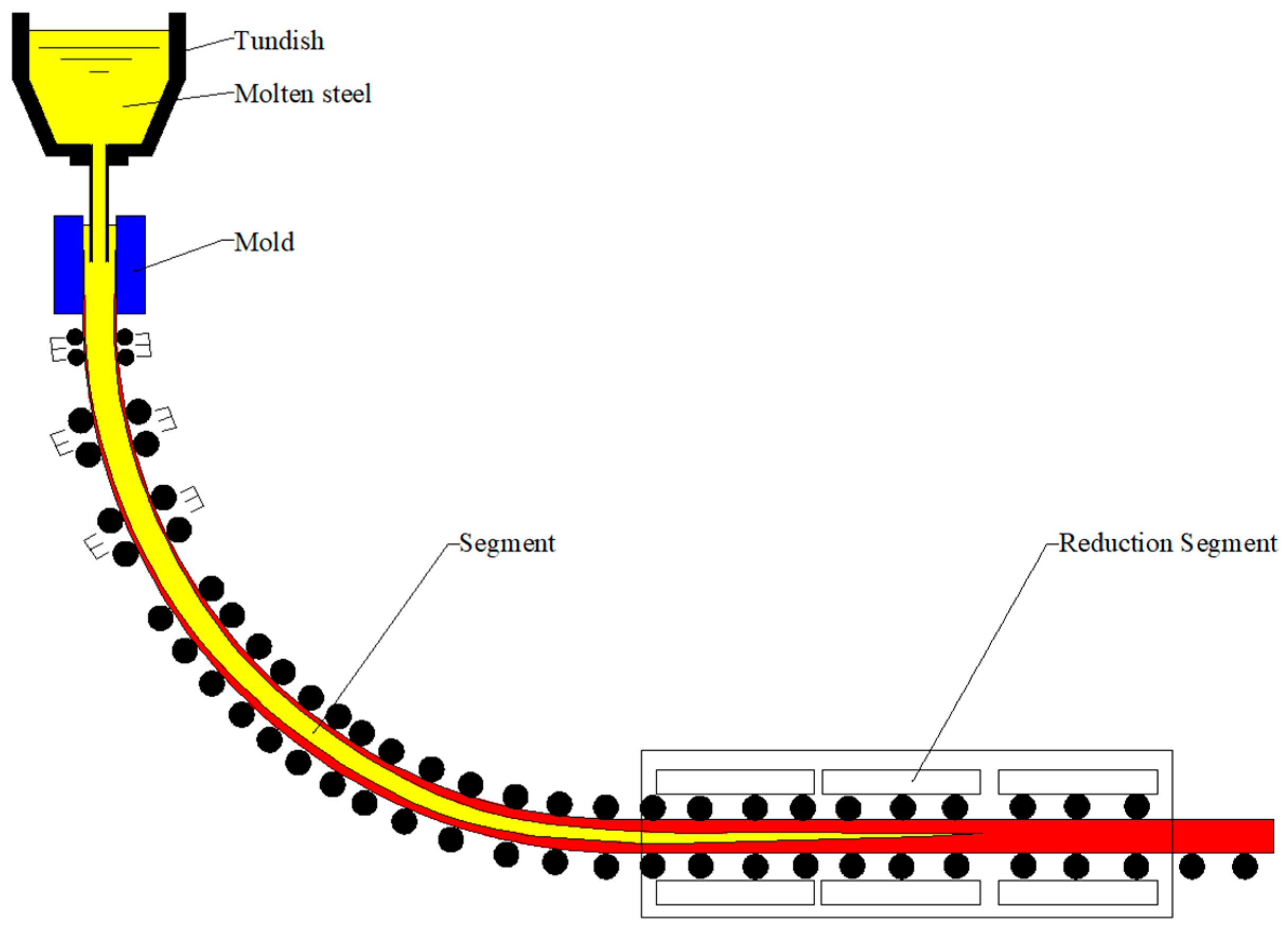
The continuous casting process involves several steps as shown in Figure 1. First, the molten steel enters the mold from the tundish and a certain thickness of the shell solidifies. The slab, with a shell of a certain thickness, then enters the caster segment from the mold. Secondary cooling is then performed until the slab is completely solidified. Next, soft reduction of the slab is performed in the caster segment by adjusting the distance between the upper and lower rollers; this adjusts the internal crystal arrangement of the slab and improves the internal quality of the slab.

There are many published studies on the prediction of continuous casting process parameters. Lait [5] developed a one-dimensional finite-difference model to calculate the temperature field and pool profile of continuously cast steel. The result obtained was reasonable for low-carbon billets over most of the mold region. Rappaz [6] described how the microscopic models of microstructure formation could be coupled to macroscopic heat flow calculations in order to predict microstructural features at the scale of the whole process. Choudhary et al. [7] developed a steady-state three-dimensional heat flow model based on the concept of artificial effective thermal conductivity. The model can be applied to various geometrical shapes of relevance to continuous casting of steel. Koric et al. [8] created an accurate multi-physics model of metal solidification at the continuum level; this model comprised of separate three-dimensional models for the thermomechanical behavior of the solidifying shell, turbulent fluid flow in the liquid pool, and thermal distortion of the mold. The model was applied to simulate continuous casting of steel. Numerical modeling is still the primary design tool used for continuous casting studies.

Artificial intelligence (AI) is a branch of the computer science discipline. AI is considered one of three cutting-edge technologies since the 1970s (those being, space technology, energy technology, and artificial intelligence). It is also considered to be one of three cutting-edge technologies of the 21st century (those being, genetic engineering, nanoscience, and artificial intelligence). AI has developed rapidly over the past three decades, has been widely used in many subject areas, and has achieved important results. AI has gradually become an independent branch of study [9]. In recent years, AI methods have been widely used in the field of intelligent manufacturing. Yang et al. [10] proposed a framework and several general guidelines for implementing big data analytics in a high-performance computing environment. AI methods have also been introduced to the field of continuous casting. Hore et al. [11] developed a model based on adaptive neural network formalism coupled with a fuzzy inference system to predict the mechanical properties of hot-rolled TRIP steel. The present model provides a predictive platform for possible application of these AI-based tools for automation, real-time process control, and operator guidance in plant operation. Liu and Gao [12] established a method for online prediction of the silicon content in blast furnace ironmaking processes. The superiority of the proposed method was demonstrated and compared with other soft sensors in terms of online prediction of the silicon content in an industrial blast furnace in China. Mahmoodkhani et al. [13] considered the friction coefficient as an input parameter in the neural network; it was optimized using an iterative method employing an equation that related the friction coefficient to the rolling force in order to rapidly predict the roll force during skin pass rolling of 980DP and 1180CP high strength steels. Tiensuu et al. [14] used statistical models to improve the dimensional accuracy of a steel plate by updating the selection of parameters for slab design. Zhang et al. [15] developed a model to predict the critical point of interfacial instability of liquid-liquid stratified flow based on the Kelvin-Helmholtz instability. The results of the water model indicated that the prediction model was correct.

Particle swarm optimization (PSO), described by Eberhart and Kennedy in 1995, is a stochastic optimization technique based on population [16]. The particle swarm algorithm mimics the clustering behavior of insects, herds, flocks, and fish groups. These groups search for food in a cooperative way. Each member of the group changes its search mode by learning from its own experience and the experience of other members of the group. Valvano et al. [17] introduced a novel decline PSO procedure. This method was used to select the optimal parameters for sound control. Similarly, PSO was used to select the optimal parameters of the support vector machine (SVM) kernel function in this paper.

The remainder of this paper is organized as follows: The data source is introduced in Section 2. The process parameters collected at the continuous casting production site were dimension reduced by PCA, as described in Section 3. The PSO-SVM is introduced in Section 4. In Section 5, the proposed model is applied to a dataset and the results are analyzed. In Section 6, the model is applied to industrial production and compared with products produced without the model. Finally, a conclusion is presented in Section 7.

2. Continuous Casting Process Parameters

2.1. Acquisition of Continuous Casting Process Parameters

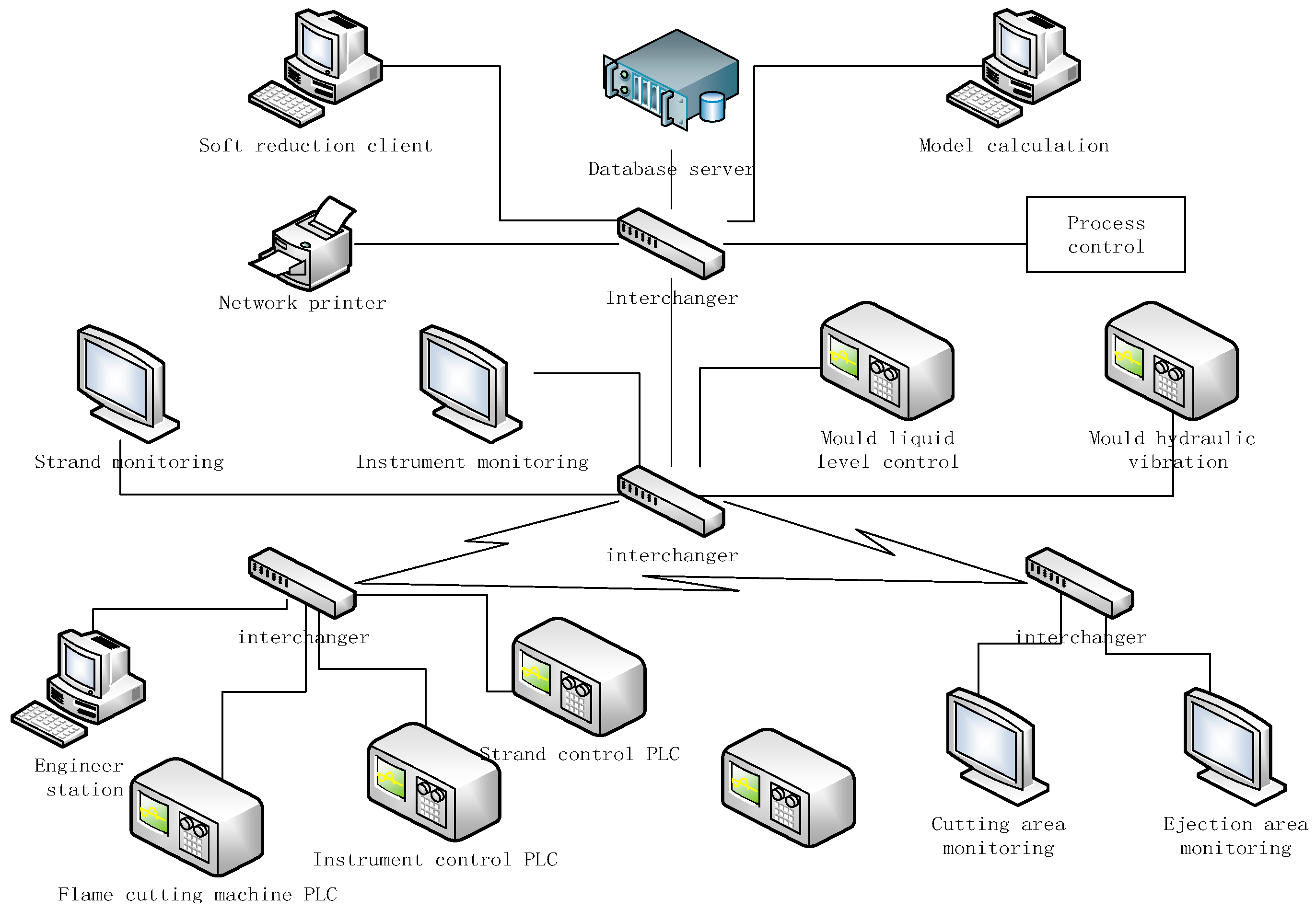
In this paper, a Chinese steel company was selected as the research object; data on the continuous casting production line was collected online from this site. The continuous casting machine under study had more than 6000 distributed sensors to record most of the process state, including the casting speed, the amount of water in each cold zone, the type of steel, and the casting temperature. Figure 2 depicts the topological structure of the continuous casting production data acquisition system. The main core equipment of the continuous casting production data acquisition system included a basic automation level Programmable Logic Controller (PLC), a man-machine interface server, a monitoring operation station, a process control-level computer database, a model application server, and a terminal client. The system collected data through the PLC controller and monitoring operation station; the data then entered the computer database. Data were analyzed and the model was updated and corrected in the model application server. Data was displayed to the operator through the terminal client; process adjustment and optimization occurred through the PLC.

In this paper, the process parameter data from the continuous casting production line were obtained with the help of field engineers; the data dimension was 6153. The process parameters included the tundish, ladle, mold, and caster segment, which were closely correlated with the roll gap value obtained; the closely related data dimension was 1020. These data were correlated with the product quality. The collection time was 1 h, the sensor recorded every 0.02 s, and the data volume was 180,000.

A correlation analysis of these process parameters was performed; the parameters that were more relevant were classified as a category. The coefficient of the association between two parameters could be obtained by:

$$r=\frac{{\displaystyle \sum _{i=1}^n(x_i-\overline{x})(y_i-\overline{y})}}{\sqrt{{\displaystyle \sum _{i=1}^n{(x_i-\overline{x})}^2\cdot {\displaystyle \sum _{i=1}^n{(y_i-\overline{y})}^2}}}}$$

(1)

where r is a correlation coefficient reflecting the relationship between two variables and the related direction of this relationship, x_i is a data point in data set X, $\overline{x}$ is the mean of X, y_i is a data point in data set Y, and $\overline{y}$ is the mean of Y.

The analyses revealed that the correlation coefficients between each process parameter were more than 0.5; many correlation coefficients were even greater than 0.8. As a result, 15 types of continuous casting process parameters were chosen, as listed in

Table 1. Process parameter names and abbreviations.

Name	Process Parameter	Name	Process Parameter
GSWD	Temperature of tundish molten steel	KMLL	Water flow of mold width surface
GRD	Overheating of molten steel	KMWD	Outlet temperature of mold width surface
LS	Pulling rate	ZMYL	Water pressure of mold narrow surface
ZDPL	Vibration frequency of mold	ZMLL	Water flow of mold narrow surface
ZDFZ	Vibration amplitude of mold	ZMWD	Outlet temperature of mold narrow surface
CDGYL	Average pressure of 18 drive rollers	ELSLL	Average flow of 18 second cold water loops
JJQYW	Mold liquid level	ELSYL	Average pressure of 18 second cold water loops
KMYL	Water pressure of mold width surface	-	-

.

2.2. Data Pre-Processing

The Pauta criterion was used to detect outliers in large monitoring data sets [18]. In this paper, the Pauta criterion was used to detect outliers in the data. The detected outliers were changed to values nearby so as not to damage the sequence of the data.

Assuming that all data were measured with the same precision and in order to obtain x₁, x₂, …, x_n, the arithmetic mean x and the residual error v_i = x_i – x (i = 1, 2, …, n) were calculated. In addition, the standard error σ was calculated using the Bessel formula. If a residual error v_b of a measured value x_b satisfied Equation (2):

$$\left|v_{\mathrm{b}}\right|=\left|x_{\mathrm{b}}-x\right|>3\mathsf{\sigma }$$

(2)

then x_b was an outlier, which contained a larger error, and thus, this value was replaced with the next value adjacent to it.

3. Dimension Reduction of Streaming Data from Multi-Source Information

3.1. Standardization of Continuous Casting Process Parameters

The continuous casting process is a complex continuous phase transition process. There are many links which affect the quality of the casting billet and there are many collected production process parameters. Therefore, the analysis of the data is particularly important. Analysis revealed that each process parameter could be a dimension of the data samples. The predicted roll gap of data was seen as a label, a group of N-dimensional process parameters was seen as an input vector x_i, $x_i\in {\Re }^{N\times 1}$, and another adjacent group of process parameters was seen as the second set of the input vector $x_i{}_{+1}$.

The unit and magnitude of the input parameters were different. Thus, the data were standardized in order to produce data in the same range for analysis under the condition of mutual equality. A linear transformation of raw data was performed to standardize the data; this mapped the result to [0, 1], according to:

$$x_{im*}=\frac{x_{im}-x_{\min }}{x_{\max }-x_{\min }}$$

(3)

where x_im was the m-dimensional process parameters of any group of input vector, x_im* was the standardization of x_im, x_max was the maximum of the sample data, and x_min was the minimum of the sample data.

3.2. Dimension Reduction of Continuous Casting Process Parameters

In this paper, in order to obtain a highly responsive roll gap value prediction model for the continuous casting caster segment, dimension reduction of the continuous casting process parameters was considered; this would reduce the operation time and the complexity of the algorithm.

The principal component contribution rate method was used to determine the number of parameters [19]. The variance contribution ratio and summation variance contribution ratio of each parameter is shown in

Table 2. Variance contribution ratio of each parameter.

NO.	Feature	Variance Contribution Ratio (%)	Summation Variance Contribution Ratio (%)
1	4.79	36.97	36.97
2	3.43	32.85	69.82
3	1.76	14.74	84.56
4	1.24	5.25	89.81
5	1.01	4.74	93.55
6	0.903	3.02	96.57
7	0.605	1.92	98.49
8	0.455	0.43	98.92
9	0.350	0.32	99.24
10	0.203	0.21	99.45
11	0.113	0.15	99.6
12	0.058	0.12	99.72
13	0.044	0.1	99.82
14	0.030	0.09	99.91
15	0.008	0.09	100.00

.

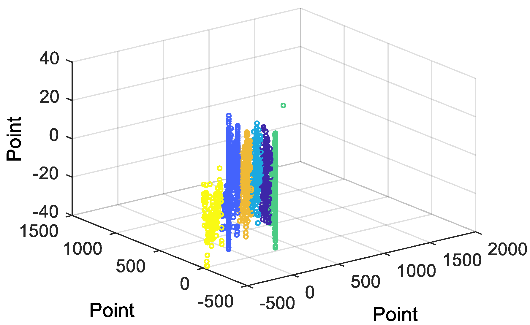
Table 2 shows that the cumulative variance contribution ratio of the first six parameters was greater than 95%. Thus, the raw data could be fully captured with six parameters.

Figure 3 shows the classification results of principal component analysis (PCA), each color represents a principal component, there are six colors in Figure 3, representing six principal components. PCA demonstrated the effect of the dimensionality specification. The PCA results demonstrated that the data was reduced from 15 dimensions to 6.

4. Establishing a Roll Gap Value Prediction Model from Multi-Source Information

4.1. PSO-SVM Model

SVM can not only solve the classification problem, but can also solve the regression problem; the basic model is the largest linear classifier defined in the feature space. SVM aims to achieve a distinction between samples by constructing a hyperplane for classification so that the sorting interval between the samples is maximized and the sample to the hyperplane distance is minimized.

Set a training data set for a feature space D = {(x₁, y₁), (x₂, y₂), …, (x_m, y_m)}, $x_i\in \mathsf{\chi }={\Re }^n$, $y_i\in y=\left\{+1,-1\right\}$, i = 1, 2, …, N, where x_i is the i-th feature vector, y_i is the class tag of x_i.

The corresponding equation of the classification hyperplane was

$$h(x)=\mathsf{\omega }\cdot x+b$$

(4)

where x was the input vector, ω was the weight, and b was the offset.

The classification decision function was

Sign (h(x))

(5)

$$\{\begin{array}{c}h(x)>0,y_i=1\\ h(x)<0,y_i=-1\end{array}$$

(6)

The support vector machine was implemented to find the ω and b when the interval between the separation hyperplane and the nearest sample point was maximized. When the training set was linearly separable, the sample points belonging to different classes could be separated by one or several straight lines with the largest interval. The maximum interval was solved by the following formula:

$$\max {\mathsf{\gamma }}_i=y_i(\frac{\mathsf{\omega }}{\Vert \mathsf{\omega }\Vert }\cdot x_i+\frac{b}{\Vert \mathsf{\omega }\Vert })$$

(7)

$$s.t.y_i(\frac{\mathsf{\omega }}{\Vert \mathsf{\omega }\Vert }\cdot x_i+\frac{b}{\Vert \mathsf{\omega }\Vert })\ge \mathsf{\gamma },i=1,2,\dots ,N$$

(8)

where γ is the geometric interval.

Thus, we could obtain the linear separable support vector machine optimization problem.

$$\underset{\mathsf{\omega },b}{\min }\frac{1}{2}{\Vert \mathsf{\omega }\Vert }^2$$

(9)

$$s.t.y_i(\mathsf{\omega }\cdot x_i+b)-1\ge 0,i=1,2,\dots ,N$$

(10)

In the actual data set, there were many specific points, making the data set linearly inseparable; in order to solve this problem, we introduced a slack variable for each sample point ξ_i ≥ 0, so that

$$y_i(\mathsf{\omega }\cdot x_i+b)\ge 1-{\mathsf{\xi }}_i$$

(11)

for each slack variable ξ_i, pay a price ξ_i, and the optimization problem becomes

$$\frac{1}{2}{\Vert \mathsf{\omega }\Vert }^2+C{\displaystyle \sum _{i=1}^N{\mathsf{\xi }}_i}$$

(12)

where C > 0 is the penalty factor.

Most of the data in the actual data were linearly inseparable. Therefore, these data could be mapped to a high-dimensional feature space through non-linear mapping, letting the non-linear problem be transformed into a linear problem. The linear indivisible problem was transformed into a linear separable problem.

Introduce kernel functions:

$$K(x_i,x_j)=\mathsf{\phi }(x_i)\cdot \mathsf{\phi }(x_j)$$

(13)

where the value of the kernel equaled the inner product of two vectors, x_i and x_j.

At this point, we obtained

$$W(\mathsf{\alpha })=\frac{1}{2}{\displaystyle \sum _{i=1}^N{\displaystyle \sum _{j=1}^N{\mathsf{\alpha }}_i{\mathsf{\alpha }}_j{y}_i{y}_{j}K(x_i,x_j)-{\displaystyle \sum _{i=1}^N{\mathsf{\alpha }}_i}}}$$

(14)

where ${\mathsf{\alpha }}_i\ge 0, i=1,2,\dots ,N$ was the Lagrangian multiplier and N was the number of samples.

In this paper, the radial basis function (RBF) was chosen as the SVR kernel function, and the expression was

$$K(x_i,x)=\exp (\frac{-{\Vert x_i-x\Vert }^2}{2g^2})$$

(15)

where g was the kernel function coefficient.

At this point, the classification function became

$$f(x)=\mathrm{sign}[{\displaystyle \sum _{i=1}^N{\mathsf{\alpha }}_i{y}_i\exp (\frac{-{\Vert x_i-x\Vert }^2}{2g^2})+b}]$$

(16)

In the SVM model, training data on the cost function and the constraint condition were known. Only the penalty factor C and the kernel function parameter g could be adjusted. When the input sample points are wrongly divided, the impact of this error can be adjusted by C; this highlights the important effect of the misclassification of sample points. The kernel function parameter g represents the kernel function parameter γ, k in the g represents the number of attributes in the input data. Thus, the hit rate of the roll gap value prediction model is governed by these two parameters [20,21,22,23,24,25,26,27,28,29].

PSO, also referred to as the particle swarm optimization algorithm or bird flock foraging algorithm, is a type of evolutionary algorithm (EA). Starting from the random solution, the optimal solution is found through iteration, and the quality of the solution is evaluated through fitness. However, the PSO algorithm rule is simpler. It searches for the global optimum by following the current optimal value. This algorithm is easy to implement, has high-precision and fast-convergence, and is suitable for solving practical problems.

PSO was used to optimize the penalty factor parameter C and kernel function parameter g in the SVM. Cross-validation of the prediction results were performed to obtain the optimal C and g so as to optimize the SVM prediction results.

Assuming that C and g are in a D-dimension target-searching space, a group was composed of m particles. The position of the i-th particle represented vector $c_i=(c_{i1},c_{i2},\dots ,c_{iD})$, i = 1, 2, …, m, whose speed was also a D-dimension vector, $g_i=(g_{i1},g_{i2},\dots ,g_{iD})$. The optimal location that the i-th particle had searched so far was $P_i=(P_{i1},P_{i2},\dots ,P_{iD})$. The optimal position in which the whole particle swarm had searched was $P_k=(P_{k1},P_{k2},\dots ,P_{kD})$. The particle updating equation was as follows:

$$g_{id}(t+1)=g_{id}(t)+h_1{r}_1(P_{id}-c_{id}(t))+h_2{r}_2(P_{kd}-c_{id}(t))$$

(17)

$$c_{id}(t+1)=c_{id}(t)+g_{id}(t+1)$$

(18)

while $g_{id}>G_{\max }$, $g_{id}=G_{\max }$;

while $g_{id}<-G_{\max }$, $g_{id}=-G_{\max }$.

In the formula, i = 1, 2, …, m; d = 1, 2, …, D. h₁ and h₂ were non-negative constants, r₁ and r₂ were uniform distribution random numbers within the range of [0, 1], c_id(t) was the current position of the i-th particle, t is the current moment, P_id was the optimal location that the i-th particle had searched so far, and g_id was the current speed of the i-th particle. $g_{id}\in [-G_{\max }, G_{\max }]$, G_max, the maximum limit speed, was a negative number.

4.2. Establishing the PSO-Roll Gap Value Prediction

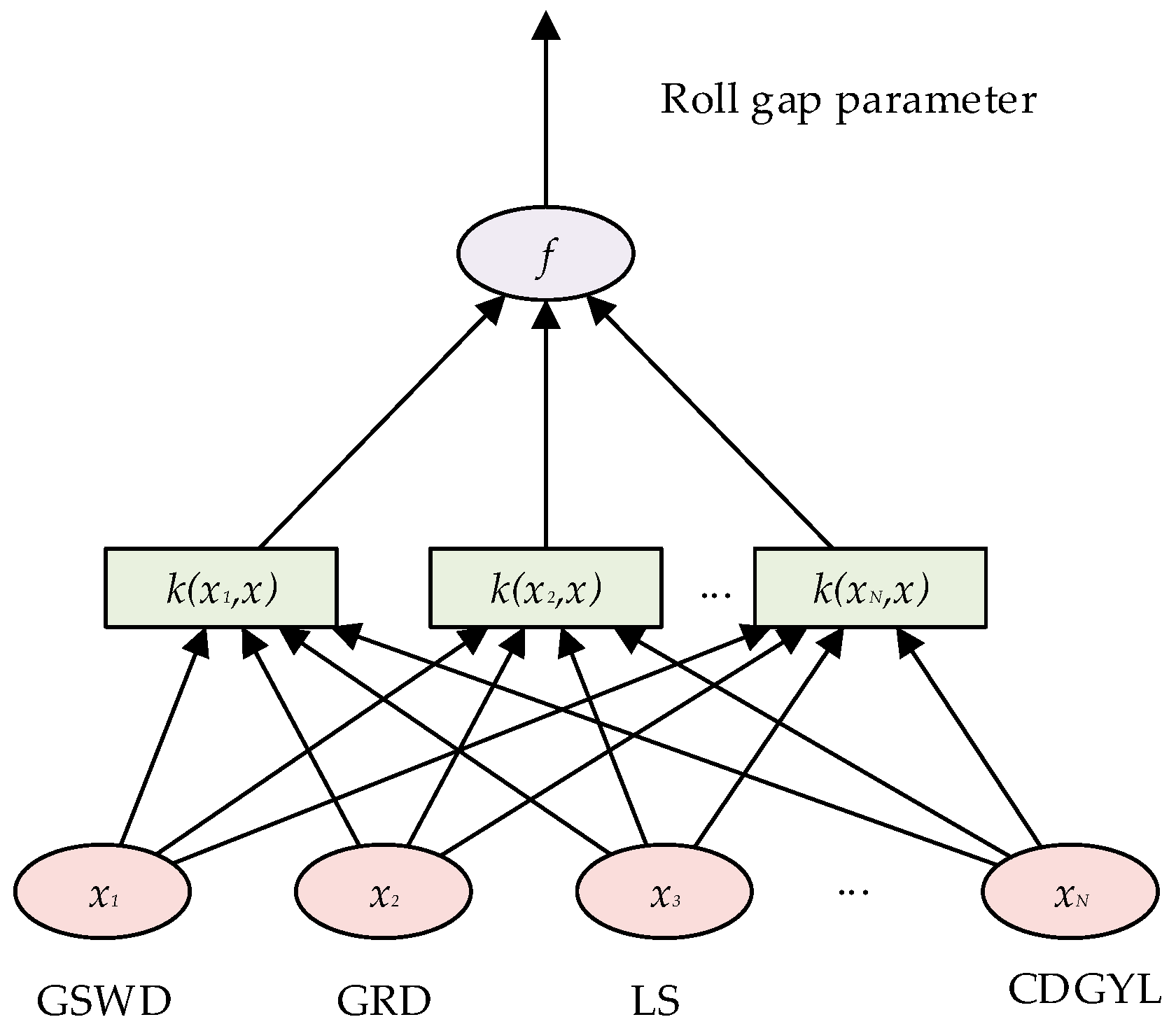
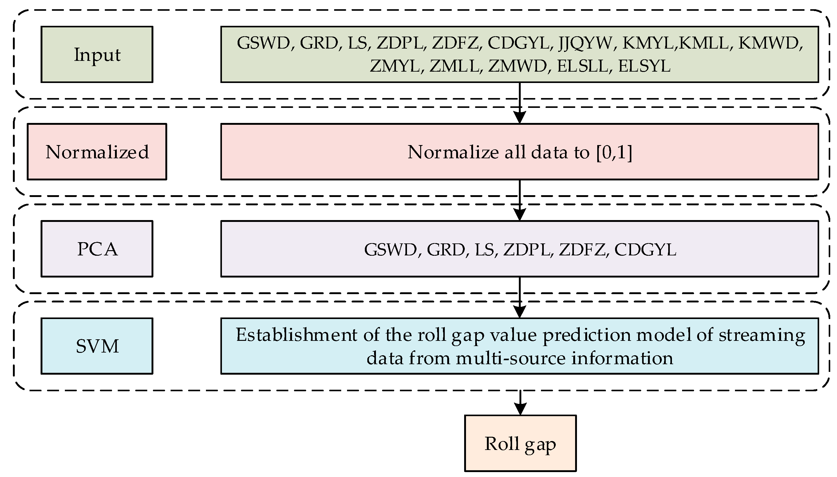
This section reports the process for establishing the PSO-SVM model. The SVM algorithm was used to establish the roll gap value prediction (RGVP) model of streaming data from multi-source information, as shown in Figure 4 and Figure 5. Six types of continuous casting process parameters comprised the input data, $k(x_1,x); k(x_2,x);\dots ;k(x_N,x)$ were the kernel functions of the SVM, and the roll gap value was the output data.

In order to enhance the accuracy of the roll gap value prediction model, PSO was used to optimize the parameters of the PSO-RGVP.

The specific steps of the PSO-RGVP were as follows:

Step 1: Pre-processing of process parameter data to obtain 15 types of process parameters.

Step 2: Standardization of process parameter data and feature reduction to obtain six types of parameters.

Step 3: Determination of the scope of C and g by PSO.

Step 4. Testing of model parameters using the method of cross validation to obtain the optimal C and g.

Step 5: Establishment of the roll gap value prediction model of streaming data from multi-source information.

Step6: Prediction of the results.

5. Experiments and Results

This section presents the results of the PSO-RGVP model and compares these results to the traditional numerical heat transfer metallurgical model; MATLAB was used to perform the experiment. This section is divided into two parts. The first was the establishment and training of the model using historical data; the second was the prediction of the test sample. Two thousand sets of process parameter data from continuous casting were collected to establish and train the model. In addition, another 500 sets of data were collected to carry out the forecast test. The experiment results are shown in

Table 3. Results of establishment and training of the model experiment.

Parameter Optimization Results	Training Time	Mean Square Deviation
C = 0.1; g = 0.1	304.8 s	97.5%

.

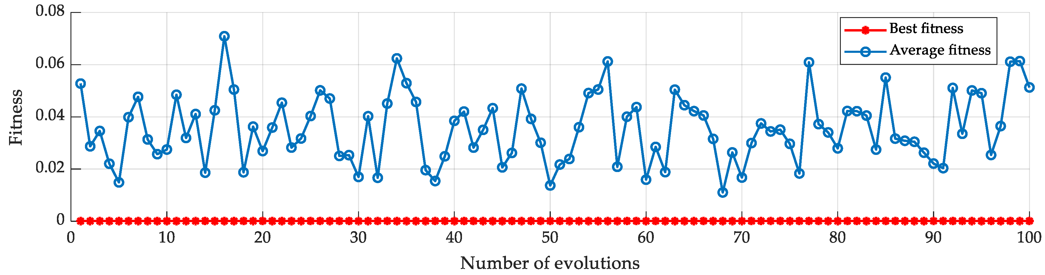
Figure 6 presents the parameter optimization results of the PSO-RGVP. When the termination generation was 100 and the population number was 20 in the PSO-RGVP, it could be concluded that the optimal penalty factor C = 0.1 and g = 0.1.

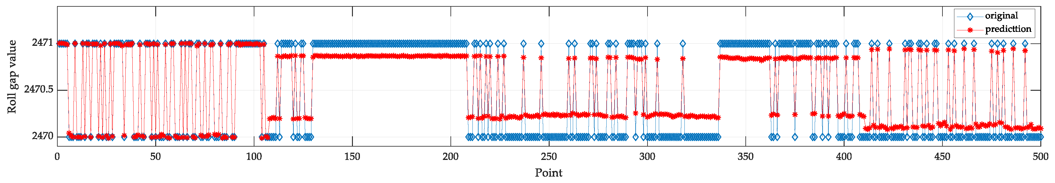
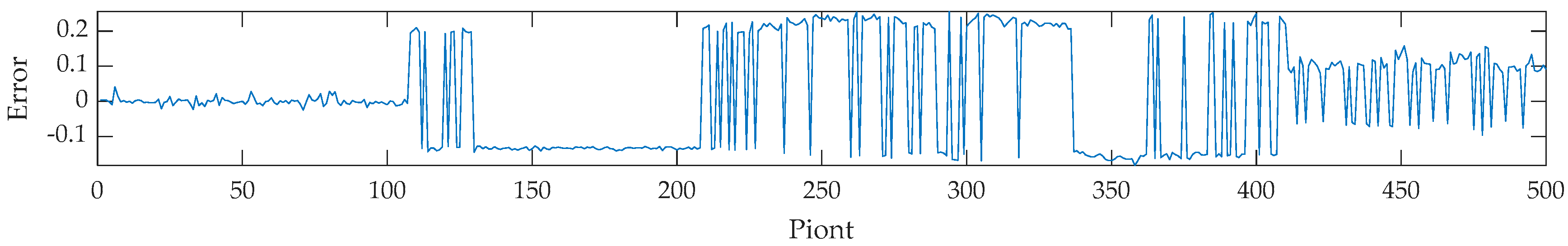
After predicting 500 sets of process parameter data that were collected with the PSO-RGVP, the predicted roll gap value was compared with the actual roll gap value, as shown in Figure 7. Relative error of prediction of the PSO-RGVP is shown in Figure 8.

The PSO-RGVP is a new way to predict the value of roll gap. The maximum relative error between the predictive value and the actual value of the method proposed in this paper was 2.5%, and the prediction accuracy was 97.5%.

6. Industrial Application

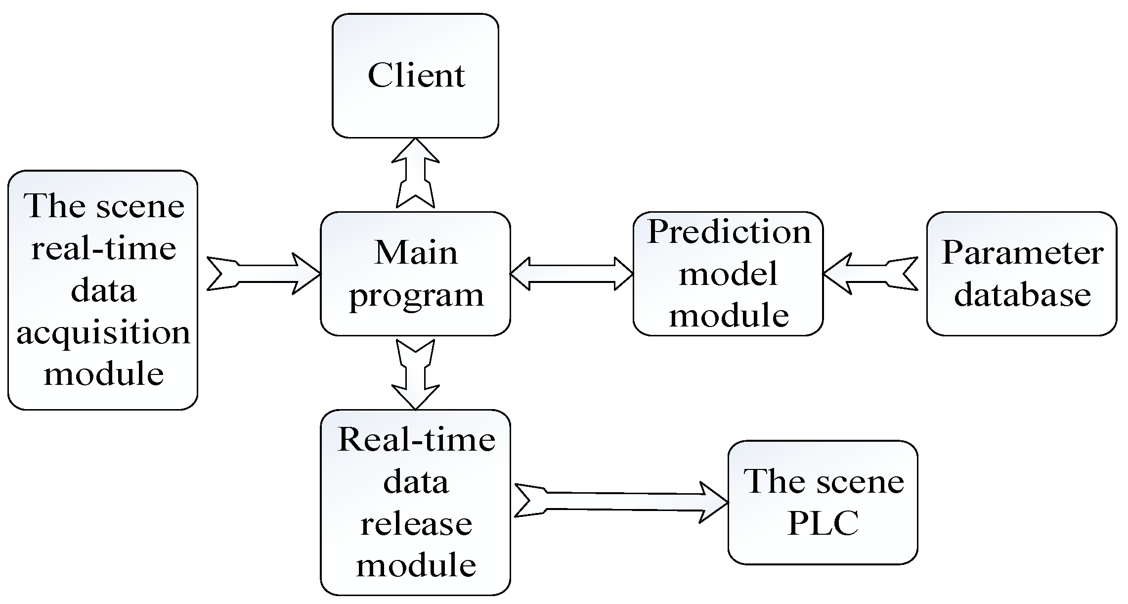
This section reports the actual application of the PSO-RGVP. Modular design was used in the system; the modular structure is shown below in Figure 9.

The test system had two main modules: The prediction model module and the main application program. Data interaction in the prediction model was achieved with the main application program; the program was structured and clearly defined in Figure 9.

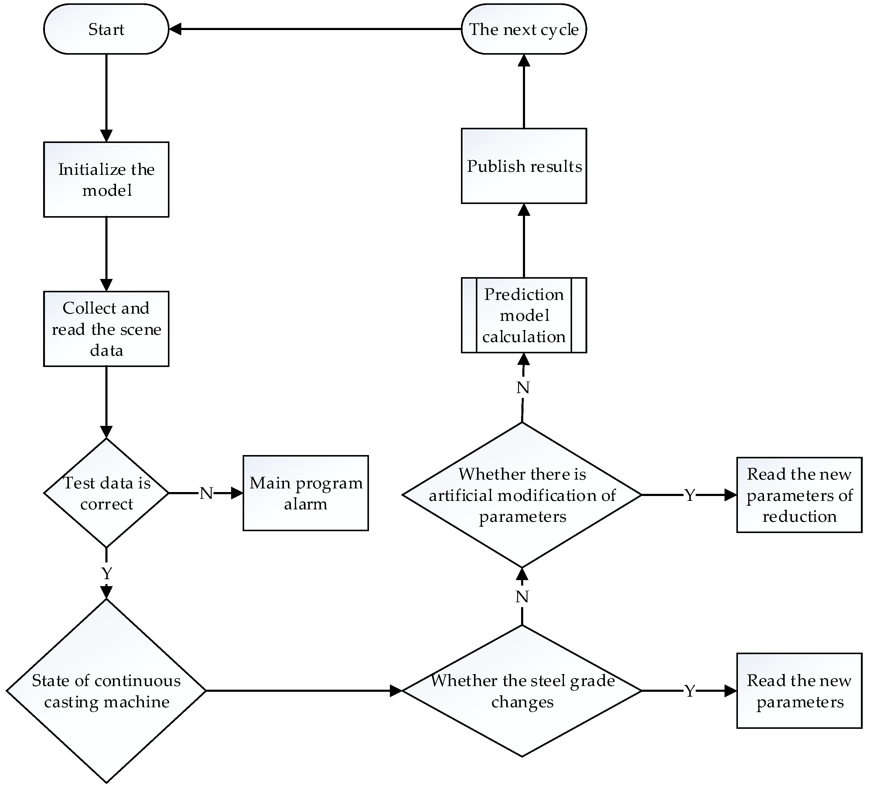
A brief operational flow chart of the test system is shown in the following diagram (Figure 10).

As shown in Figure 10, after initializing the model, the system first acquired the real-time process parameters and filtered for correctness of the process parameters. Through the identification of real-time data, the system obtained the status of the continuous casting machine at the time and decided whether to carry out the roll gap adjustment strategy. Through the identification of the type of steel, the system read the total rolling reduction, the rolling interval, the rolling distribution, etc. The prediction model was used to obtain the roll gap prediction value, which was then released.

The prediction data was imported into the test system for trial production, then casting was performed and the quality of the slab was observed.

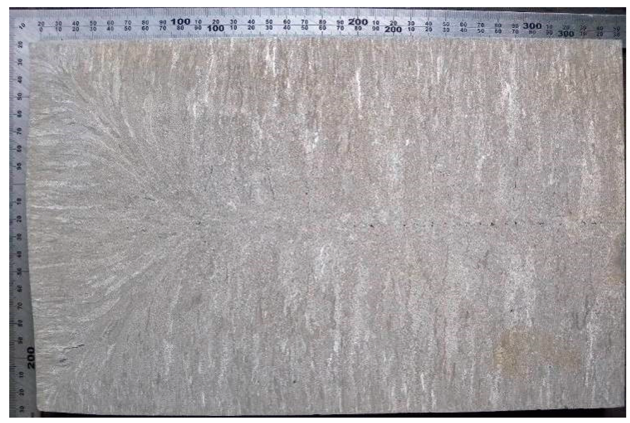
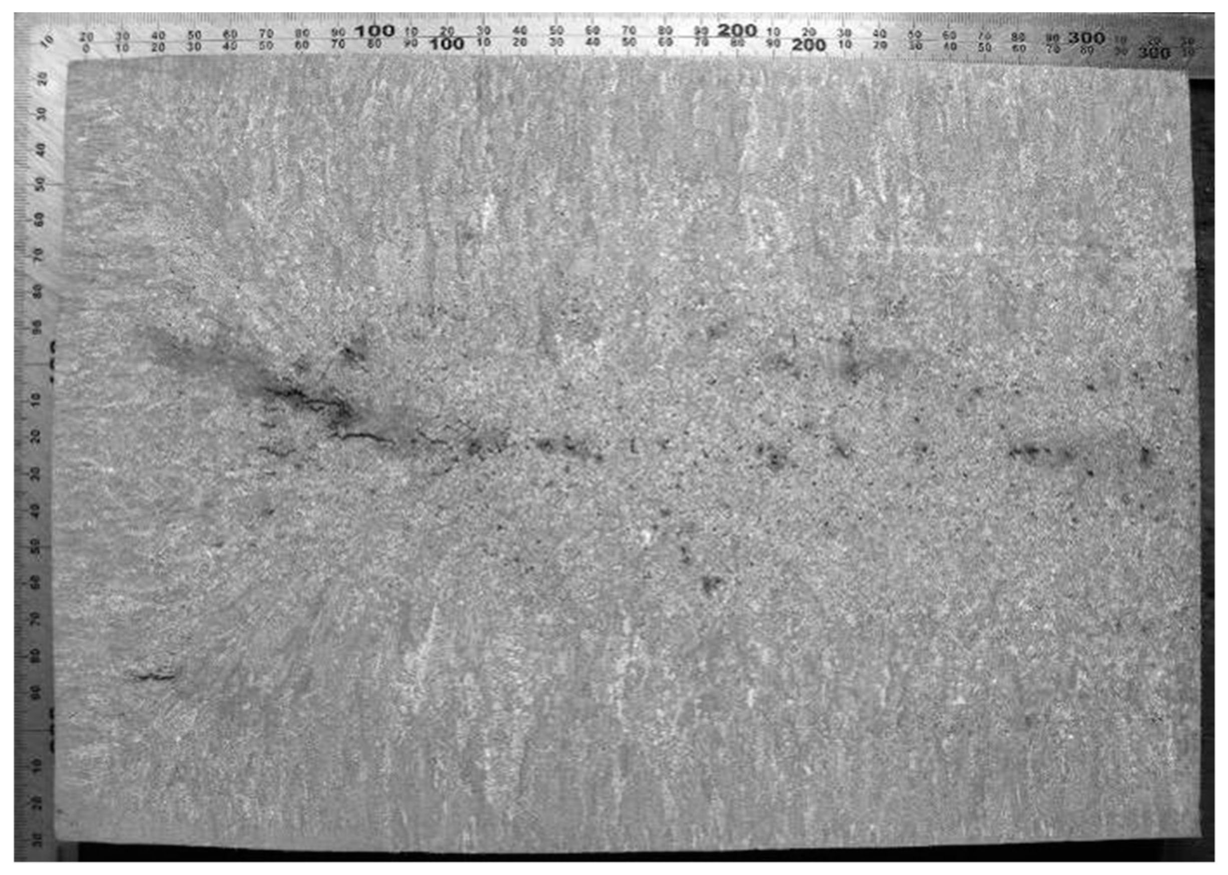
In order to verify the application of the model, the center segregation and center porosity of the slab, before and after use of the model, were analyzed by macroscopic examination. In particular, the continuous casting machine was compared before and after use of the model for the production of steel for Q235; the section size was 230 × 1350, the cast speed was 1.30 m/min, and the total reduction was 4 mm. The results of macroscopic examination were determined according to Chinese metallurgical standards. The results are reported in

Table 4. Comparison of quality rating.

Serial Number	Section Size (mm × mm)	Centre Segregation	Centre Porosity	Intermediate Cracks	Triangle Area Cracks
Without proposed model	230 × 1350	B1.0	2.0	1.5	1.5
Proposed model	230 × 1350	C0.5	1.0	1.0	0.5

and in Figure 11 and Figure 12.

Figure 11 and Figure 12 show the macrosegregation examination of the two methods: The proposed model and the traditional method. The macrosegregation sample was cut from the continuous casting slab. After polishing and pickling the surface, it was photographed under a low-power microscope. This was the main approach used to check the internal quality of a slab. It was obvious that under the same production conditions, the slab produced under the proposed model only had very few intermediate cracks; the quality rating of center segregation was C0.5; center porosity was 1.0; intermediate cracks was 1.0; triangle area cracks was 0.5. According to the quality of the intermediate cracks produced by the proposed model, the center segregation and center porosity in the slab were greatly reduced. After using the proposed model, the center segregation and center porosity in the slab were greatly reduced. In addition, the proposed model greatly reduced the labor intensity and maintenance time and improved the maintenance efficiency for production.

The results indicate that the roll gap prediction model proposed in this paper has a short computational time, can accurately predict the roll gap, and allows for real-time prediction and adjustment during production. The findings from the industrial application of this model demonstrate its accuracy. Thus, the roll gap value prediction efficiency is greatly increased in the proposed model. In this study, 2000 sets of data were collected to establish and train the model. In addition, another 500 sets of data were collected to carry out the forecast test. The prediction accuracy was 97.5%. This showed that the PSO-RGVP was superior for prediction of the roll gap value.

7. Conclusions

In this paper, a new prediction approach, PSO-RGVP, was proposed. Multi-source information process parameters from the continuous casting process were excavated and analyzed, and PSO was used for global optimization of an adaptive prediction model for the roll gap value of the caster segment; SVM was used for the prediction of the roll gap. This method takes into account the mutual influence and restriction of the multi-source information process parameters in the actual production process; the model parameters were obtained quickly and accurately, and adaptive prediction of the roll gap value was achieved. The experimental results confirmed the efficiency of the PSO-RGVP, because actual data was used. PSO-RGVP provides a new approach for the prediction of the roll gap value.

References

- Ataka, M. Rolling technology and theory for the last 100 years: The contribution of theory to innovation in strip rolling technology. ISIJ Inter. 2015, 55, 89–102. [Google Scholar] [CrossRef]
- Ge, S.; Isac, M.; Guthrie, R.I.L. Progress of strip casting technology for steel; historical developments. ISIJ Inter. 2012, 52, 2109–2122. [Google Scholar] [CrossRef]
- Tacke, K.H.; Schwinn, V. Recent developments on heavy plate steels. Stahl Eisen 2005, 125, 55. [Google Scholar]
- Wolf, M.M. History of Continuous Casting. In Proceedings of the 75th Steelmaking Conference, Toronto, ON, Canada, 5–8 April 1992; pp. 47–101. [Google Scholar]
- Lait, J. Mathematical modelling of heat flow in the continuous casting of steel. Ironmak. Steelmak. 1974, 1, 90–97. [Google Scholar]
- Rappaz, M. Modeling of microstructure formation in solidification processes. Int. Mater. Rev. 1989, 34, 93–123. [Google Scholar] [CrossRef]
- Choudhary, S.K.; Ganguly, S. Morphology and segregation in continuously cast high carbon steel billets. ISIJ Inter. 2007, 47, 1759–1766. [Google Scholar] [CrossRef]
- Koric, S.; Hibbeler, L.C.; Liu, R.; Thomas, B.G. Multiphysics model of metal solidification on the continuum level. Numer. Heat Transfer, Part B-Fundam. 2010, 58, 371–392. [Google Scholar] [CrossRef]
- Nilsson, N.J. Principles of Artificial Intelligence; Morgan Kaufmann Publishers: Burlington, MA, USA, 2014. [Google Scholar]
- Yang, Y.; Cai, Y.D.; Lu, Q.; Zhang, Y.; Koric, S.; Shao, C. High-Performance Computing Based Big Data Analytics for Smart Manufacturing. In Proceedings of the ASME 2018, the 13th International Manufacturing Science and Engineering Conference, College Station, TX, USA, 18–22 June 2018. [Google Scholar]
- Hore, S.; Das, S.K.; Banerjee, S.; Mukherjee, S. An adaptive neuro-fuzzy inference system-based modelling to predict mechanical properties of hot-rolled TRIP steel. Ironmak. Steelmak. 2016, 44, 656–665. [Google Scholar] [CrossRef]
- Liu, Y.; Gao, Z. Enhanced just-in-time modelling for online quality prediction in BF ironmaking. Ironmak. Steelmak. 2015, 42, 321–330. [Google Scholar] [CrossRef]
- Mahmoodkhani, Y.; Wells, M.A.; Song, G. Prediction of roll force in skin pass rolling using numerical and artificial neural network methods. Ironmak. Steelmak. 2016, 44, 281–286. [Google Scholar] [CrossRef]
- Tiensuu, H.; Tamminen, S.; Pikkuaho, A.; Röning, J. Improving the yield of steel plates by updating the slab design with statistical models. Ironmak. Steelmak. 2016, 44, 577–586. [Google Scholar] [CrossRef]
- Zhang, L.; Li, Y.; Wang, Q.; Yan, C. Prediction model for steel/slag interfacial instability in continuous casting process. Ironmak. Steelmak. 2015, 42, 705–713. [Google Scholar] [CrossRef]
- Eberhart, R.; Kennedy, J. A New Optimizer Using Particle Swarm Theory. In Proceedings of the MHS’95, the Sixth International Symposium on Micro Machine and Human Science, Nagoya, Japan, 4–6 October 1995; pp. 39–43. [Google Scholar] [CrossRef]
- Valvano, S.; Orlando, C.; Alaimo, A. Design of a noise reduction passive control system based on viscoelastic multilayered plate using PDSO. Mech. Syst. Sig. Process. 2019, 123, 153–173. [Google Scholar] [CrossRef]
- Zhang, M.; Yuan, H. The Pauta criterion and rejecting the abnormal value. J. Zhengzhou Univ. Tech. 1997, 1, 84–88. [Google Scholar]
- Martinez, A.M.; Kak, A.C. PCA versus LDA. IEEE Trans. Pattern Anal. Mach. Intell. 2001, 23, 228–233. [Google Scholar] [CrossRef]
- Cervantes, J.; Garcia-Lamont, F.; Rodriguez-Mazahua, L.; Lopez, A.; Ruiz-Castilla, J.; Trueba, A. PSO-based method for SVM classification on skewed data sets. Neurocomputing 2017, 228, 187–197. [Google Scholar] [CrossRef]
- Chiang, J.H.; Hao, P.Y. A new kernel-based fuzzy clustering approach: Support vector clustering with cell growing. IEEE Trans. Fuzzy Syst. 2003, 11, 518–527. [Google Scholar] [CrossRef]
- Fang, Y.; Hu, C.; Liu, L.; Zhang, X. Breakout prediction classifier for continuous casting based on active learning GA-SVM. China Mech. Eng. 2016, 27, 1609–1614. [Google Scholar] [CrossRef]
- Gaudioso, M.; Gorgone, E.; Labbe, M.; Rodriguez-Chia, A.M. Lagrangian relaxation for SVM feature selection. Comput. Oper. Res. 2017, 87, 137–145. [Google Scholar] [CrossRef] [Green Version]
- Zhang, G.Z.; Sun, J. Application of fuzzy control on the caster segment’s gap control of slab continuous casting machine. Electr. Drive 2009, 39, 51–53. [Google Scholar]
- Jain, A.K.; Duin, R.P.W.; Mao, J. Statistical pattern recognition: A review. IEEE Trans. Pattern Anal. Mach. Intell. 2000, 22, 4–37. [Google Scholar] [CrossRef]
- Muscat, R.; Mahfouf, M.; Zughrat, A.; Yang, Y.Y.; Thornton, S.; Khondabi, A.V.; Sortanos, S. Hierarchical fuzzy support vector machine (SVM) for rail data classification. IFAC Papersonline 2014, 47, 10652–10657. [Google Scholar] [CrossRef]
- Refan, M.H.; Dameshghi, A.; Kamarzarrin, M. Improving RTDGPS accuracy using hybrid PSOSVM prediction model. Aerosp. Sci. Technol. 2014, 37, 55–69. [Google Scholar] [CrossRef]
- Wang, J.-S.; Chiang, J.-C. A cluster validity measure with Outlier detection for support vector clustering. IEEE Trans. Syst. Man Cybern. Part B Cybern. 2008, 38, 78–89. [Google Scholar] [CrossRef] [PubMed]
- Wei, J.; Zhang, R.; Yu, Z.; Hu, R.; Tang, J.; Gui, C.; Yuan, Y. A BPSO-SVM algorithm based on memory renewal and enhanced mutation mechanisms for feature selection. Appl. Soft Comput. 2017, 58, 176–192. [Google Scholar] [CrossRef]
Figure 1.
Continuous casting process.
Figure 2.
Topological structure of the continuous casting production data acquisition system.
Figure 3.
Dimensionality reduction results of Principal Component Analysis (PCA).
Figure 4.
Roll gap value prediction model of streaming data from multi-source information. f is the output of the model.
Figure 5.
Common computational architecture of roll gap value prediction model.
Figure 6.
Parameter optimization results of PSO.
Figure 7.
Prediction results of PSO-RGVP.
Figure 8.
Relative error of prediction of the PSO-RGVP.
Figure 9.
System modular structure diagram.
Figure 10.
Test system calculation process.
Figure 11.
Macrosegregation examination of results of the proposed model.
Figure 12.
Macrosegregation examination of the results of the traditional method.