Effect of an Electrically-Conducting Wall on Transient Magnetohydrodynamic Flow in a Continuous-Casting Mold with an Electromagnetic Brake

Abstract

Large eddy simulation (LES) of transient magnetohydrodynamic (MHD) turbulent flow under a single-ruler electromagnetic brake (EMBr) in a laboratory-scale, continuous-casting mold is presented. The influence of different electrically-conductive boundary conditions on the MHD flow and electromagnetic field was studied, considering two different wall boundary conditions: insulating and conducting. Both the transient and time-averaged horizontal velocities predicted by the LES model agree well with the measurements of the ultrasound Doppler velocimetry (UDV) probes. Q-criterion was used to visualize the characteristics of the three-dimensional turbulent eddy structure in the mold. The turbulent flow can be suppressed by both configurations of the experiment’s wall (electrically-insulated and conducting walls). The shedding of small-scale vortices due to the Kelvin–Helmholtz instability from the shear at the jet boundary was observed. For the electrically-insulated walls, the flow was more unstable and changed with low-frequency oscillations. However, the time interval of the changeover was flexible. For the electrically-conducting walls, the low-frequency oscillations of the jets were well suppressed; a stable double-roll flow pattern was generated. Electrically-conducting walls can dramatically increase the induced current density and electromagnetic force; hence they contribute to stabilizing the MHD turbulent flow.

1. Introduction

Continuous casting (CC) has become one of the most important production processes in the steel industry. The molten steel from the ladle flows through the tundish into a mold and then freezes against the water-cooled copper mold, forming a solidified shell. High casting speed has been widely used to reduce the production cost and to enhance the productivity. Therefore, the molten steel flows in the mold with intense turbulence, especially along the hot jets that escape from the submerged entry nozzle (SEN) ports. The hot jets are very likely to cause a “breakout” accident near the impingement points on the narrow walls [1]. In addition, the turbulent flow of molten steel plays a key role in the slab quality, since it influences the growth of a solid shell, causes slag entrapment, the floatation of bubbles and non-metallic inclusions [2,3,4,5,6].

Electromagnetic braking (EMBr) is considered an effective flow control technology to maintain a stable “double-roll” flow pattern in the CC mold. Several commercial configurations of EMBr have been successfully used in slab casting, such as local EMBr [7,8,9], single-ruler EMBr [10,11,12,13,14], and double-ruler EMBr [15,16,17,18,19]. The flow of the electrically-conductive molten steel in the magnetic fields generates an electromagnetic force opposing the motion, and thus should be self-stabilizing. Experimental studies using low-melting-point metallic melts on the magnetohydrodynamic (MHD) flow have been reported by some researchers [8,10,19,20,21]. Harada et al. [8] investigated the effect of different types of EMBrs on the fluid flow using the mercury model. A plug-like flow in the liquid pool can be developed by the level magnetic field, but not by the local magnetic field. Zhang et al. [19] studied the flow pattern of mercury in a flow control mold (FC-mold) under various magnetic distributions and flux densities. Optimum conditions of the upper and lower magnetic flux densities were present based on the free surface fluctuation and the flow recirculation profiles. Considering the risks of mercury, the ternary alloy GaInSn was used by the Helmholtz Zentrum Dresden-Rossendorf (HZDR) to investigate the impact of a level magnetic field on the discharging jet [11,20,21]. Some advanced measurement technology, such as ultrasound Doppler velocimetry (UDV) and contactless inductive flow tomography (CIFT), were used to reconstruct the flow structure of the liquid metal under the influence of one or multiple magnetic fields. However, the interaction between the diverse magnetic fields and the turbulent flow appears to be a rather complex phenomenon, so that it deserves further investigation.

Computational fluid dynamics (CFD) allows a deeper inside view into the MHD flow in the mold. Extensive numerical simulations have been carried out considering various magnetic field configurations and flow parameters [9,12,13,14,15,16,17,18,22,23,24,25]. Miao et al. [22] reconstructed the peculiar phenomenon of the excitation of non-steady, non-isotropic, large-scale flow perturbations caused by the application of an external direct current (DC) magnetic field using a Reynolds-averaged Navier–Stokes (RANS)-SST turbulence model. Li et al. [23] studied the influence of the vertical electromagnetic brake (V-EMBr) on the steel/slag interface behavior using the k-ε turbulence model; the immersion depth and the port angle are not as sensitive as those in the other type of EMBrs. Some transient studies based on large eddy simulation (LES), by Thomas et al. [12,13,15,24], reveal deeper insights into the fundamental nature of the turbulent flow and electromagnetic effects, such as the stability of the jet, surface-level fluctuations, flow profiles, and argon bubble transport. Liu et al. [16] investigated the transient fluid flow and inclusion transport under various EMBr arrangements and flux densities. A significant effect on the removal rate of inclusions was found, especially for larger ones. Vakhrushev et al. [25] compared the capability of the commercial software ANSYS Fluent and the open-source CFD package OpenFOAM on the modeling of the MHD flow.

In the CC mold, the molten steel freezes against the water-cooled copper mold, forming a solid shell. The whole area can be divided into three parts: the liquid pool, mushy zone, and the solid shell. The electrical conductivity of the solidified shell is higher than that of the molten steel. An electrically-conducting wall is an essential parameter affecting the turbulent flow in the presence of an external magnetic field [11,20,21,26,27,28]. Recently, Timmel et al. [11,20,21] studied the effect of the electrically-conducting wall on the turbulent flow using two brass plates attached to the inner walls to emulate the solidified shell in the real process. The existence of a conducting wall can stabilize the flow by suppressing the unsteady low-frequency oscillation of the jets. The effect on stability has been confirmed with some numerical simulations [13,22]. However, few researchers study the details of electromagnetic field distribution (current density and Lorentz force) in both the liquid pool and solidified shell. Such an investigation is important to attain deeper insight into the fundamental nature of the MHD flow and to optimize the design of EMBr devices.

The current work presents a mathematical model for investigating the transient MHD turbulent flow under a single-ruler EMBr in a laboratory scale CC mold. The influence of different electrically-conductive boundary conditions on the turbulence flow and electromagnetic fields is considered. The numerical results are validated with measurements made in the mini-LIMMCAST facility at HZDR [11].

2. Mini-LIMMCAST Experiments

The mini-LIMMCAST facility is a small-scale CC mold employed at HZDR for investigating liquid metal flow and related transport processes. The eutectic alloy Ga₆₈In₂₀Sn₁₂ was chosen as the operating fluid at room temperature. A detailed description and schematic view of the experimental facility can be found in the previous work by Timmel et al. [11].

Table 1. Physical properties and operation conditions.

Parameter	Value
Mold width/thickness	140 mm/35 mm
Mold length	330 mm
Nozzle diameter	10 mm
Nozzle port angle	0°
Nozzle port height/width	18 mm/8 mm
Submergence depth of nozzle	72 mm
Casting speed	1.35 m/min
Velocity at nozzle inlet	1.4 m/s
Dynamic viscosity of GaInSn	0.00216 kg/m·s
Density of GaInSn	6360 kg/m3
Electrical conductivity of GaInSn	3.2 × 106 1/Ω·m
Magnetic permeability of GaInSn	1.257 × 10−6 H/m
Wall thickness at wide face (brass)	0.5 mm
Electrical conductivity of brass	15 × 106 1/Ω·m
Maximum magnetic field strength	310 mT
$\mathrm{Reynolds}\mathrm{number},\mathrm{Re}$	41,222
$\mathrm{Hartmann}\mathrm{number},Ha$	417
Stuart number, N	5

shows the physical properties and operating conditions in the experiment. The rectangular mold was made of plexiglass. The melt was supplied from a tundish to the mold through a plexiglass tube as SEN and flowed through a U-bend channel into a catchment tank. Then an electromagnetic pump conveyed the melt from the tank back into the tundish. During this process, the liquid levels of both tundish and mold were monitored using a laser distance sensor. A DC magnetic field with a maximum field strength of B = 310 mT was installed perpendicular to the flow direction near the SEN ports along the wide wall of the mold. The distribution of the measured magnetic field [12,14] along the vertical casting direction is shown in Figure 1, and was considered in the current study. To simulate the solidified shell in the real mold, the inner walls of the wide mold faces were covered with thin brass plates with a thickness of 0.5 mm. The melt velocity along the midsection of the narrow face of the mold was measured by an ultrasound Doppler velocimeter (UDV) using a maximum of ten sensors. The first sensor was placed at z = 0.24 m on the mid-plane of the narrow wall, and the subsequent sensors were placed at 10 mm intervals below the first one.

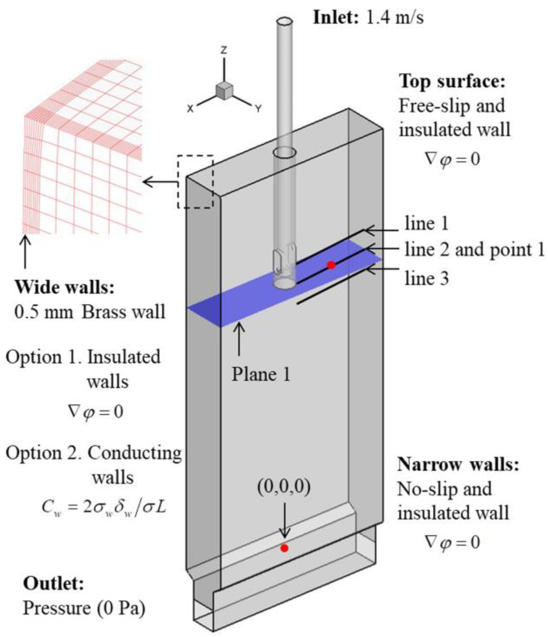
3. Computational Model

The primary objective of this work was to study the effect of different electrically-conductive boundary conditions on the transient MHD phenomena and electromagnetic field. The numerical simulation was performed using the commercial solver FLUENT 14.5. The electrical potential method was used to solve the MHD equations. It is valid for low magnetic Reynolds numbers, which are mostly valid for the CC process. The turbulent flow in the SEN and mold is modeled by the LES model.

3.1. Fluid Flow Field

The continuous and Navier–Stokes equations were solved:

$$\nabla ·\overline{u}=0$$

(1)

$$\rho \frac{\partial \overline{u}}{\partial t}+\rho \left(\overline{u}·\nabla \right)\overline{u}=-\nabla p+\nabla ·\left[\left(\mu +{\mu }_t\right)\left(\nabla \overline{u}+\nabla {\overline{u}}^T\right)\right]+F_L$$

(2)

where $\rho$, $\overline{u}$ and $p$ are the density, velocity vector, and pressure. $\mu$ is the dynamic viscosity of the fluid. The superscript “$-$” represents filtered. The external magnetic field affects the fluid flow through the electromagnetic force $F_L$. The turbulent viscosity ${\mu }_t$ was calculated based on the Smagorinsky sub-grid scale model [29]:

$${\mu }_t=\rho {\left(C_s\Delta \right)}^2\sqrt{2{\Vert S\Vert }^2}$$

(3)

where $C_s=0.1$ is the Smagorinsky constant. $\Delta =V_{cell}^{1/3}$ is the filter width. $S$ is the rate-of-strain tensor given by $S=\frac{1}{2}\left(\nabla \overline{u}-\nabla {\overline{u}}^T\right)$.

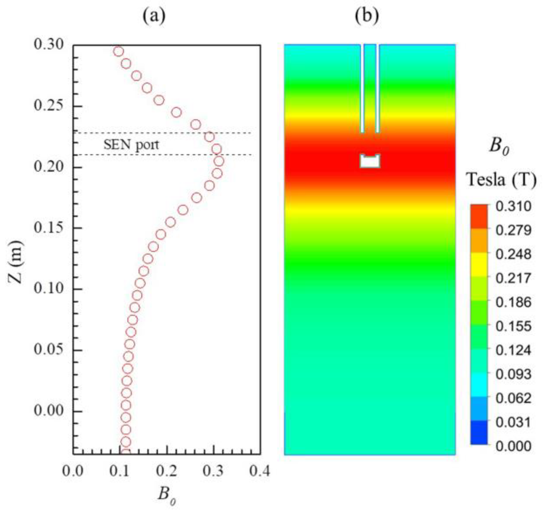
3.2. Electromagnetic Field

Lorenz’s law was used to calculate the electromagnetic force $F_L$:

$$F_L=J\times B$$

(4)

The symbol $B(0,B_0,0)$ denotes the applied external magnetic field. $J$ is the induced current density, which was calculated by the electrical potential approach as follows:

$$J=\sigma \left(E+\overline{u}\times B\right)$$

(5)

where $E$ is the electric field, which can be written in the form of $E=-\nabla \phi$. Based on the charge conservation condition, $\nabla ·J=0$, was used to obtain the equation for the electric potential $\phi$.

$${\nabla }^2\phi =\nabla ·\left(\overline{u}\times B\right)$$

(6)

3.3. Numerical Details

The geometry, material properties, and boundary conditions (Figure 2) were set according to the mini-LIMMCAST facility at HZDR [11]. Both the liquid metal and the conductive side walls (0.5 mm brass plates) at the wide faces of the mold were included. The whole domain was divided into 3.94 million cells. The grid along the mold walls was refined to catch the better resolution of the electromagnetic field inside the brass plates and the Hartmann layers. The velocity and turbulence parameters at the inlet were obtained based on the casting speed. A free-slip boundary condition with zero potential gradients was applied on the top surface of the meniscus. Along the walls of the SEN and mold, the no-slip boundary condition was employed. At the outlet of the domain, a fully-developed flow was assumed, where the static pressure was set to zero.

The boundary condition for the electric potential along the walls is given by

$$\frac{\partial \phi }{\partial n}={\left(\overline{u}\times B\right)}_{boundary}·n$$

(7)

where $n$ is the unit vector normal to the boundary. For an insulated boundary, $\partial \phi /\partial n=0$, no electric current can penetrate into the wall. For a conducting boundary, where the electric current can penetrate into the wall, a specified potential is assigned at the boundary. The current density can then be calculated from Equation (6).

In the real CC process, because of the existence of the solidified slag film between the slab and copper mold, no electrical current flows inside the copper mold. Considering the fact that the electrical conductivity of the solidified shell is higher than that of the molten steel, the electrical conductivity and thickness of the solidified shell were taken into account to assess the magnetic field effect on the turbulent flow in the liquid pool of the mold. In the current work, the cases of electrically-insulated walls and conducting walls were compared. The wall conductance ratio was defined as:

$$C_w=2\frac{{\sigma }_w{\delta }_w}{\sigma L}$$

(8)

where ${\sigma }_w$ and ${\delta }_w$ denote the electrical conductivity and the thickness of the electrically-conducting wall, respectively. $L$ is the characteristic length, which takes the thickness of the mold.

For the GaInSn physical model, the wall conductance ratio for brass was 0.134, which is almost the same value for a real steel caster with a mold thickness of 90 mm assuming a thickness of the solidified shell of 5 mm [14]. For the cases of electrically-insulated walls, the wall conductance ratio was zero.

The computational cost for the unsteady MHD turbulence flow is normally orders of magnitudes higher than that for steady state calculations in terms of memory and CPU time. Therefore, the unsteady calculation of the LES was started based on a steady state initial flow fields of the k-ε model. The transient MHD flow was calculated for 30 s and the data were monitored for every time step. Statistical data were collected and averaged over the entire time.

4. Results and Discussion

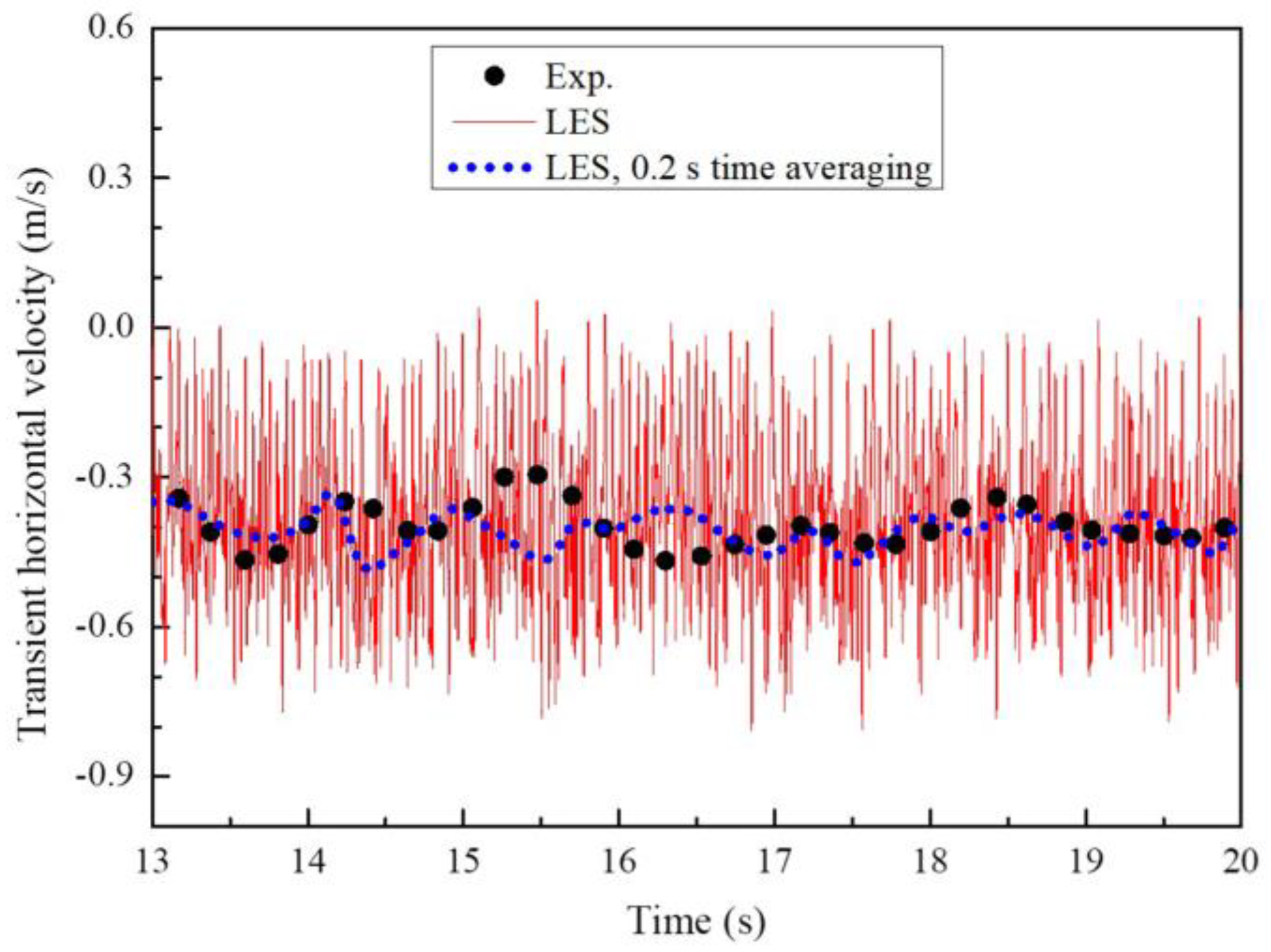
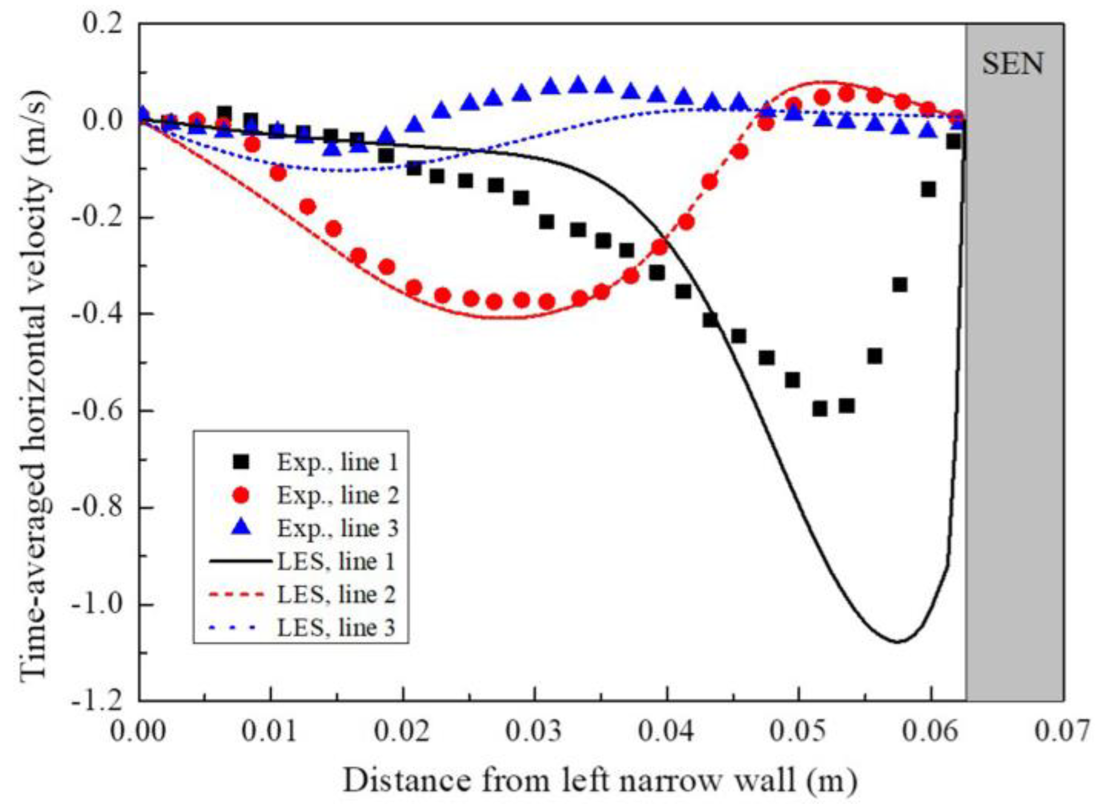
4.1. Comparison between Simulations and Measurements

The transient horizontal velocity history calculated by the LES model was compared with the measurements of the UDV probes [11,14] at point 1 (Figure 2: x = −0.041 m, y = 0 m, z = 0.2 m) in the jet region, as shown in Figure 3. The minus sign of the velocity represents the negative direction of x. The differences in fluctuation frequency and amplitude between them were caused by the different sampling rates. For the LES model, the monitoring data was collected at every time step (0.001 s), so a higher frequency and amplitude were obtained than those of the measurements, which had a frequency of 5 Hz for these measuring sensors [30]. In order to compare closely with the measurements, a 0.2 s time average was performed on the calculated signal. The two methodologies agree very well with each other for the low-frequency time-averaged signals. In other words, the transient fluctuation behavior of the MHD flow in the mold was well-captured by the LES model.

The UDV measurements of horizontal velocity on three horizontal lines, 90, 100 and 110 mm from the top surface (Figure 2), for the case with electrically-conducting walls in the GaInSn physical model [11] and the LES predictions are compared in Figure 4. For the current case, the model predictions with conducting walls agree with the measurements, except an overestimation of the maximum velocity close to the SEN on line 1. Timmel et al. [11] have reported that the UDV measurements might be inaccurate near the SEN and the narrow walls, because of the low vertical spatial resolution and the interaction between the ultrasonic transducer beam and solid walls. Thus, the time-averaged behavior of the MHD flow in the mold was also well-captured by the LES model.

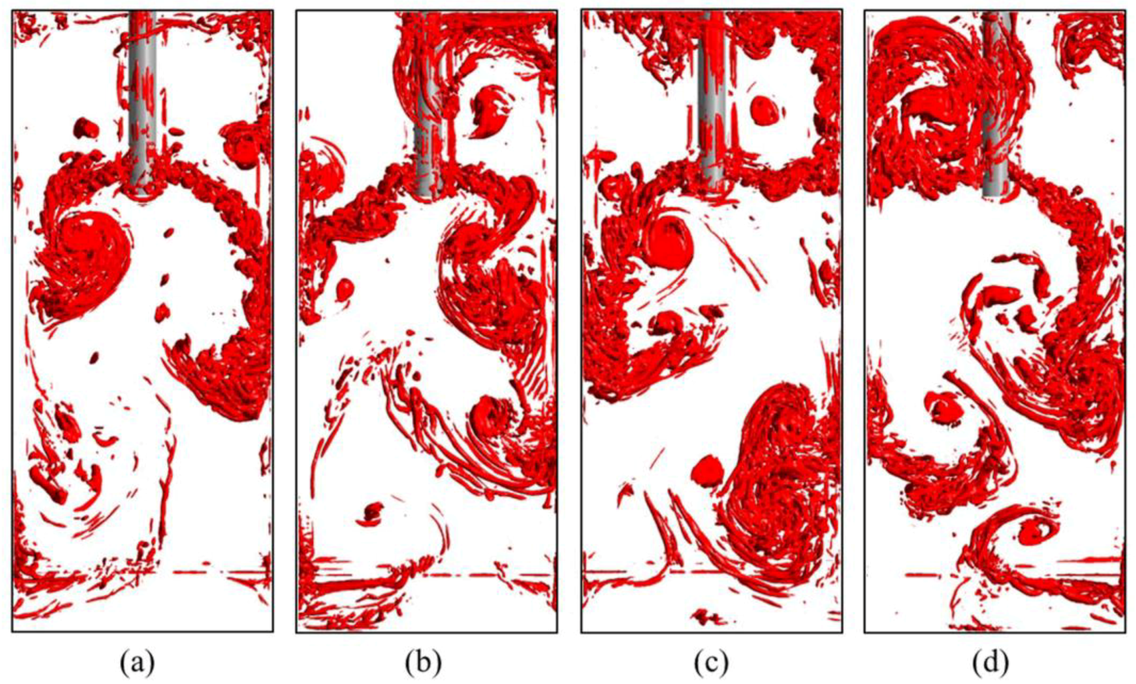
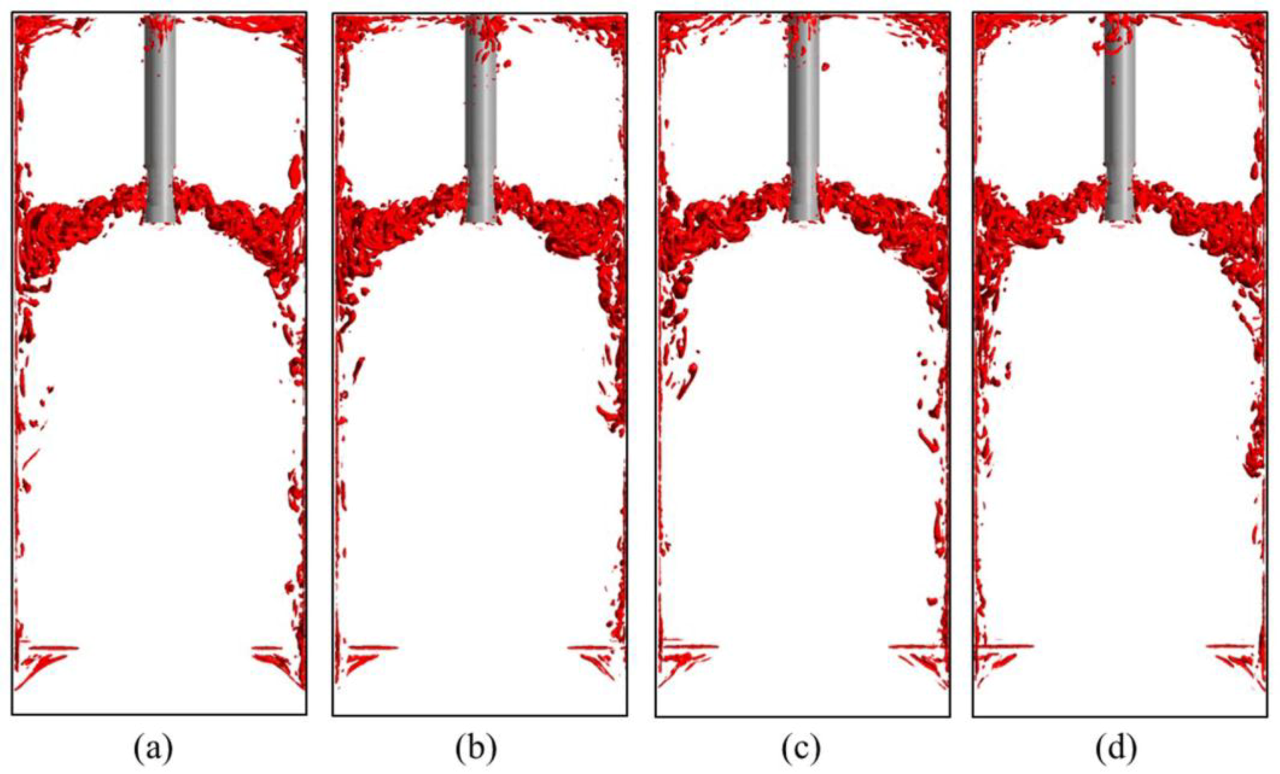
4.2. Instantaneous Flow Characteristics

In order to visualize the characteristic three-dimensional eddy structure, snapshots of the instantaneous (t = 20 s) distributions of the iso-surfaces of the Q-criterion [31] are shown in Figure 5. The Q-criterion was calculated using the following relation:

$$Q=\frac{1}{2}\left({\Omega }^2-S^2\right)$$

(9)

where $S$ is the rate-of-strain tensor, and $\Omega$ is the vorticity tensor.

All the simulations were calculated using the same mesh and the same time step. The value of the Q-criterion was 500 1/s². Apparently, the large-scale eddy structure occupied almost the entire mold for the case without EMBr, as shown in Figure 5a. This implies that the turbulent flow in the mold was strong. However, the highly turbulent nature of flow might lead to the risk of an uneven solidified shell (even breakout), the entrainment of mold slag, and other quality problems. For the situation of electrically-insulted walls, in Figure 5b, the turbulent flow was suppressed in most areas of the mold. It is interesting to note that the flow field in the mold seemed to be significantly asymmetric. The entire left jet bent upward to the top surface, forming a large upper recirculation zone on the left of the SEN. In contrast, the right jet bent downward to form a large lower recirculation zone on the right of the mold. Some disconnected and discontinuous eddy structures can be seen in other positions, which might be shed from the previous vortex structures. In the case of the electrically-conducting walls, in Figure 5c, almost all the highly turbulent nature of the flow was suppressed, except along the jets. A typical double-roll flow pattern was observed, and the eddy structures were more stable and symmetric compared with the case of electrically-insulted walls.

Figure 6 shows snapshots of the instantaneous eddy structures for the case applying EMBr together with electrically-insulated walls at sequence. Many pronounced large-scale vortex structures can be clearly seen inside the mold, containing various small-scale vortices between them. The distribution is asymmetric and dependent on low-frequency oscillations. The flow pattern is not stationary. In addition, some small-scale vortices were shed from the big ones in the left lower recirculation region of the mold, as shown in Figure 6a. This shedding of small-scale vortices may be attributed to the Kelvin–Helmholtz instability from the shear at the jet boundary. This is a constant phenomenon, especially in the lower recirculation region. The low-frequency oscillations of the jets were also observed/measured by the experiments in the mini-LIMMCAST facility at HZDR [11,22]. The DC magnetic field in combination with the electrically-insulated walls triggered this asymmetric flow, which was a consequence of the asymmetric nature of the MHD turbulence.

In order to analyze the periodicity of the low-frequency oscillations of the jets, the transient horizontal velocity history at point 1 was monitored, as illustrated in Figure 7. The phenomenon of alternating peaks and valleys represents the oscillation of the jets, which is a kind of periodical motion. However, the time interval for the changeover is flexible in that it can be affected by other parameters such as casting speed, the structure of SEN, gas injection, etc.

Figure 8 shows the sequence of instantaneous eddy structures for the case applying EMBr together with electrically-conducting walls at different times. The low-frequency oscillations of the jets were well suppressed; a stable double-roll flow pattern was generated, which is in favor of producing steel with a good quality. Except for the shear flow at the jet boundary, the shear flow on the walls plays another important role in the creation of vortices, as shown in the figures, along with the narrow walls of the mold. Interestingly, some linear vortex structures appeared near the bottom of the mold. These linear vortex structures were produced by the shear along the shrinking wall corners, as shown in Figure 2. The results indicate that the geometry of the SEN and mold, even the shape profile of the solidified front, may contribute to the formation of turbulent eddy structures.

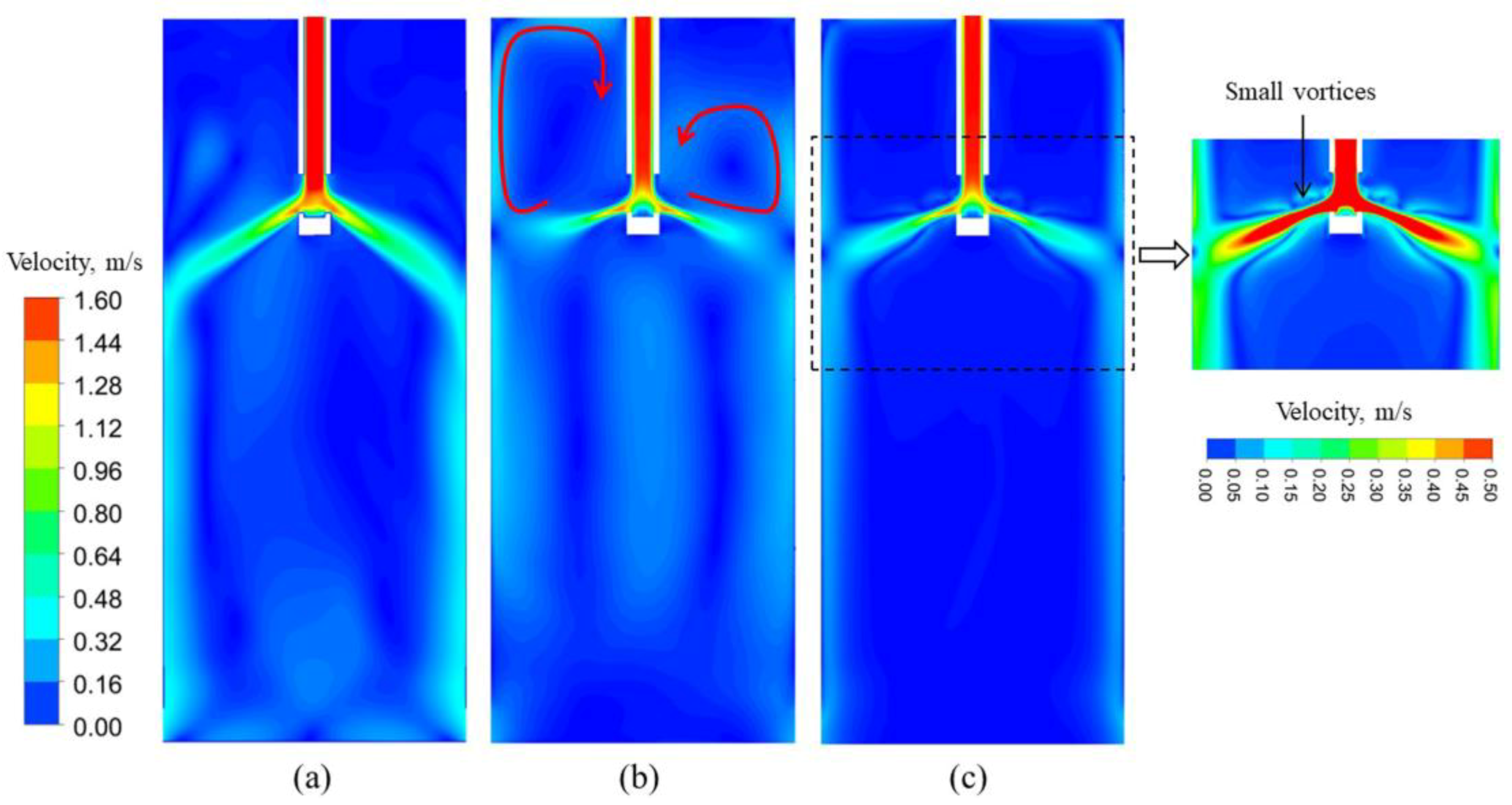
4.3. Time-Averaged Velocity and Electromagnetic Field Characteristics

Figure 9 shows the contour plots of the time-averaged velocity profiles under various magnetic field configurations. In the absence of EMBr, in Figure 9a, the fluid is discharged from the SEN port as a strong jet impinging on the narrow wall of the mold. The liquid metal jet is then split into two vertical streams, creating the upper and lower recirculation zone. The intensity of the downward jet was much stronger than the upward one. The influence of the magnetic field with electrically-insulated walls on the flow pattern can be seen in Figure 9b. The intensity of the jet was suppressed by the DC magnetic field. The impingement points on the narrow walls of the mold moved significantly upward to the top surface, which led to a remarkable enforcement of the upper recirculation flow. A significant backflow toward the top surface can be observed just above the jet, but the backflows on two sides of the SEN are still asymmetric. For the case of electrically-conducting walls, in Figure 9c, significant changes of the liquid metal flow pattern can be observed. The turbulent flow in the center of the mold was significantly suppressed. It is interesting to observe that some small quasi-two-dimensional vortex structures were generated along the directions of the magnetic field as recirculation areas near the jet, as shown in the right-hand subfigure in Figure 9c. As mentioned above, it may be the result of the MHD turbulence in the case of electrically-conducting walls.

Another important purpose of this work was to study the influence of different electrically-conductive boundary conditions on the electromagnetic field. Figure 10 shows the contours of the time-averaged, induced electrical current density on plane 1, obtained under different electrically-conductive boundary conditions. For the case of EMBr with electrically-insulated walls, Figure 10a, no induced electrical current could flow through the solid brass region. In another case, the electrical current could go directly through the electrically-conducting walls. Therefore, the induced electrical current could be seen in the solid brass regions. The value of the induced electrical current density in the solid brass was much larger than that of the liquid GaInSn, because the conductivity of brass is much higher. The peak value of the induced electrical current density in the center of the liquid pool for the case of EMBr with electrically-conducting walls was 1.67 times more than that case of EMBr with electrically-insulated walls, as shown in the inserted close-up in Figure 11. This is due to the higher velocity in the center for the case of the electrically-conducting walls. The induced electrical current density near the walls in the liquid pool was much larger than that in the center, as shown in Figure 10 and Figure 11. An explanation can be found in Figure 12, in the analysis of the vectors of the induced current on plane 1. More induced electrical current can be observed near the walls in the liquid pool.

Figure 13 shows the contours of the time-averaged electromagnetic force on plane 1 obtained under different electrically-conductive boundary conditions. Based on Lorenz’s law (Equation (4)), the electromagnetic force depends on the induced electrical current and magnetic field. The external DC magnetic field intensity (maximum = 0.31 T) was much larger than the induced magnetic field (maximum = 6 × 10⁻⁴ T). Therefore, the intensity and path of the induced electrical current had a distinct influence on the resulting electromagnetic force. The value of the electromagnetic force was directly related to the liquid metal velocity, and the direction was essentially opposite to that of the liquid metal velocity. This is the mechanism of the electromagnetic brake. Therefore, the stronger electromagnetic force can be seen along the liquid metal jets. The electromagnetic force along the jets in the case of electrically-conducting walls is larger than that of electrically-insulated walls. In relation to the higher induced current density (Figure 11), the electromagnetic force near the walls in the liquid pool was much larger than that in the center, as shown in Figure 14. The electromagnetic force in the solid region in the case of electrically-insulated walls was zero, but it was very large (up to 2.4 × 10⁻⁵ N/m³) for electrically-conducting walls. However, the electromagnetic force in this region did not impact the behavior of the fluid region.

5. Conclusions

A large eddy simulation (LES) model was applied to investigate the transient magnetohydrodynamic (MHD) turbulent flow under a single-ruler EMBr in a laboratory scale continuous-casting mold. The following conclusions can be drawn:

(1)

Both the transient and time-averaged horizontal velocities predicted by the LES model agreed well with the measurements of the UDV probes. The transient fluctuation and time-averaged behaviors of the MHD flow in the mold was well captured by the current LES model.

(2)

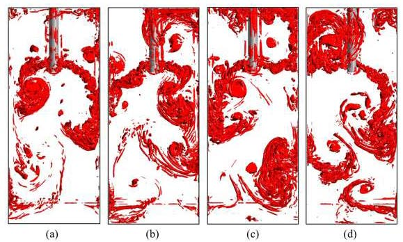
The Q-criterion was used to visualize the characteristics of the three-dimensional turbulent eddy structure. Many pronounced large-scale vortex structures could be clearly seen inside the mold, containing various small-scale vortices between them. The highly turbulent nature of the flow could be suppressed by both configurations of the mold (electrically-insulated and conducting walls). The shedding of small-scale vortices due to the Kelvin–Helmholtz instability of the shear at the jet boundary was observed.

(3)

For the configuration of the EMBr with electrically-insulated walls, the flow was more unstable and changed with low-frequency oscillations. The phenomenon of alternating peaks and valleys in the velocity represents the oscillation of the jets as a kind of periodical motion. The time interval for the changeover was flexible.

(4)

For the configuration of EMBr with electrically-conducting walls, the low-frequency oscillations of the jets were well suppressed. Consequently, a stable double-roll flow pattern was generated.

(5)

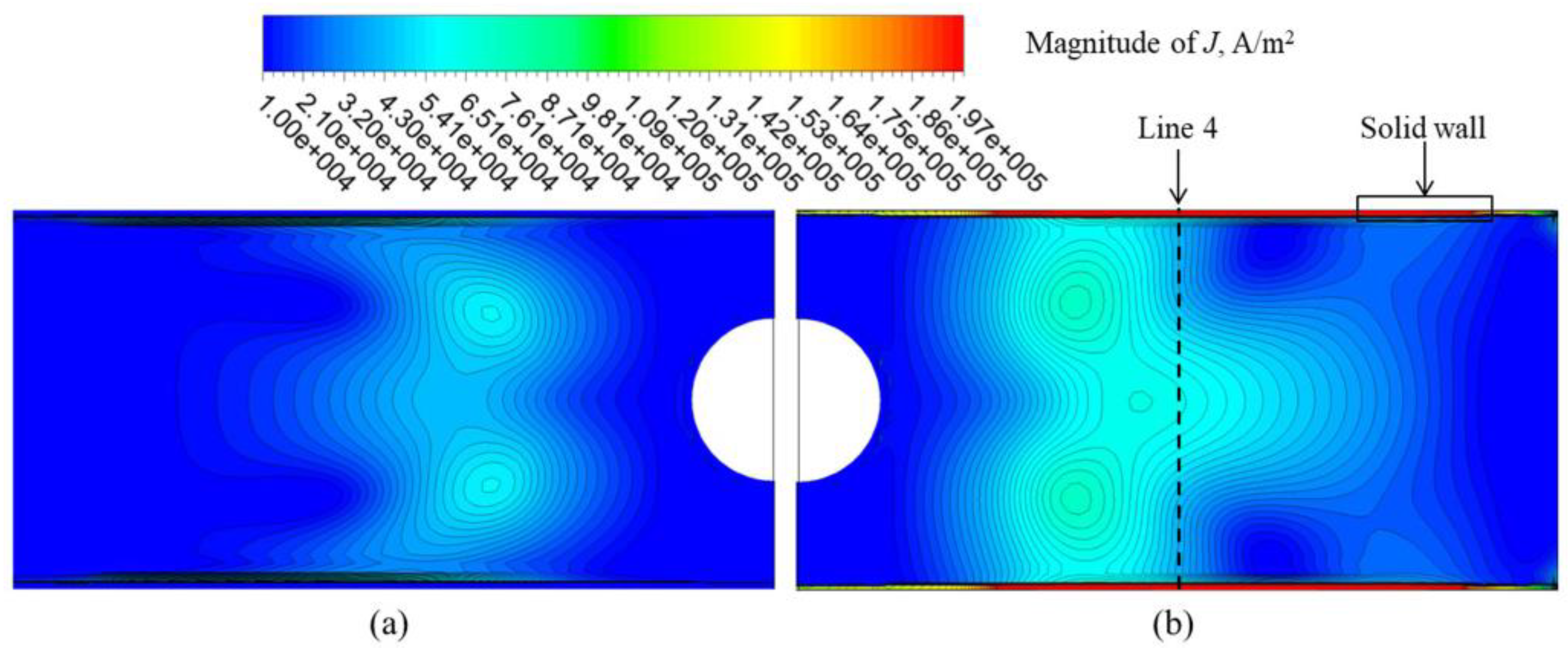
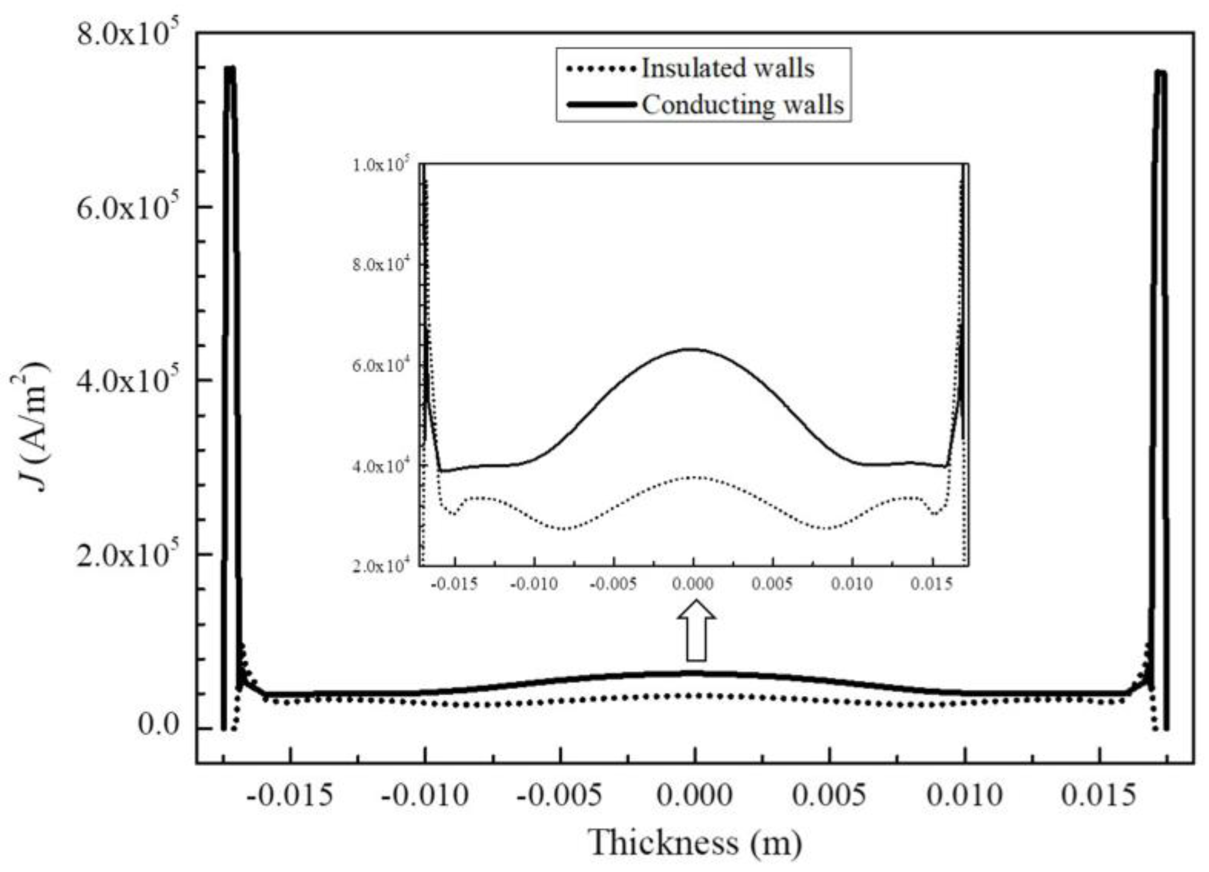
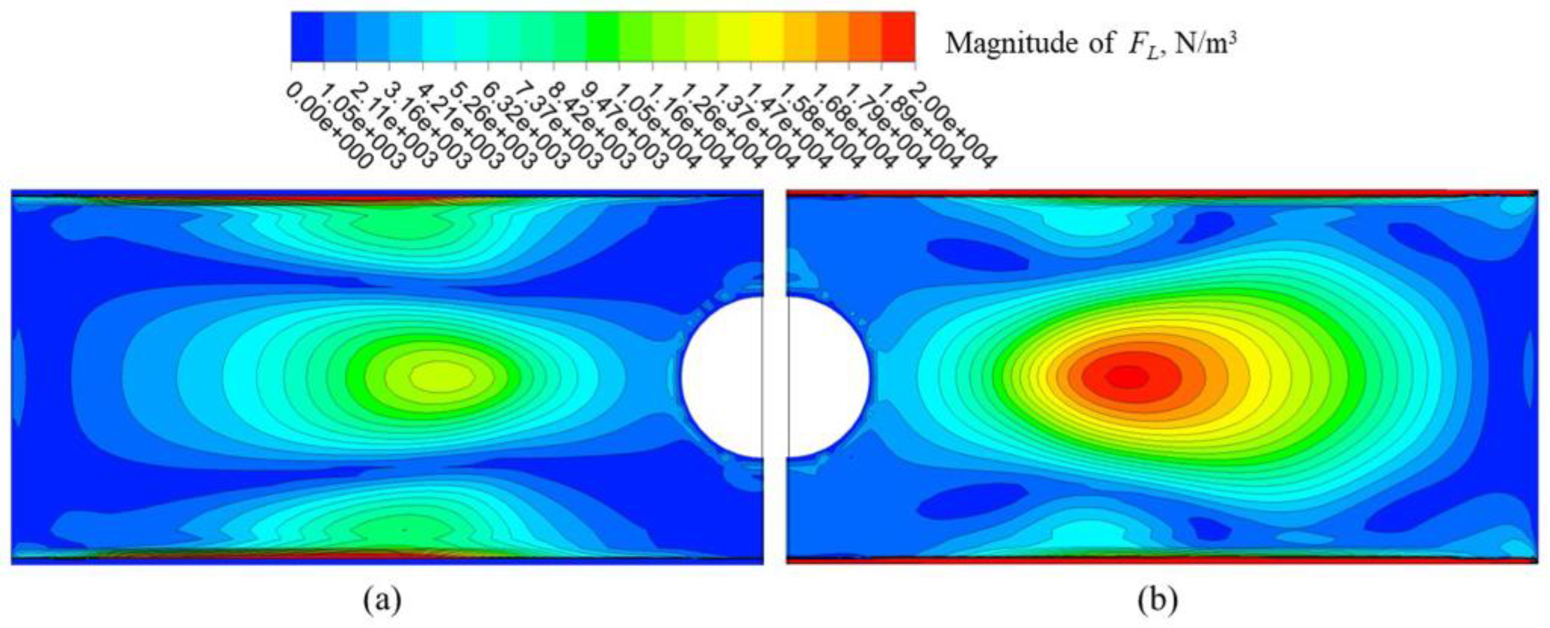
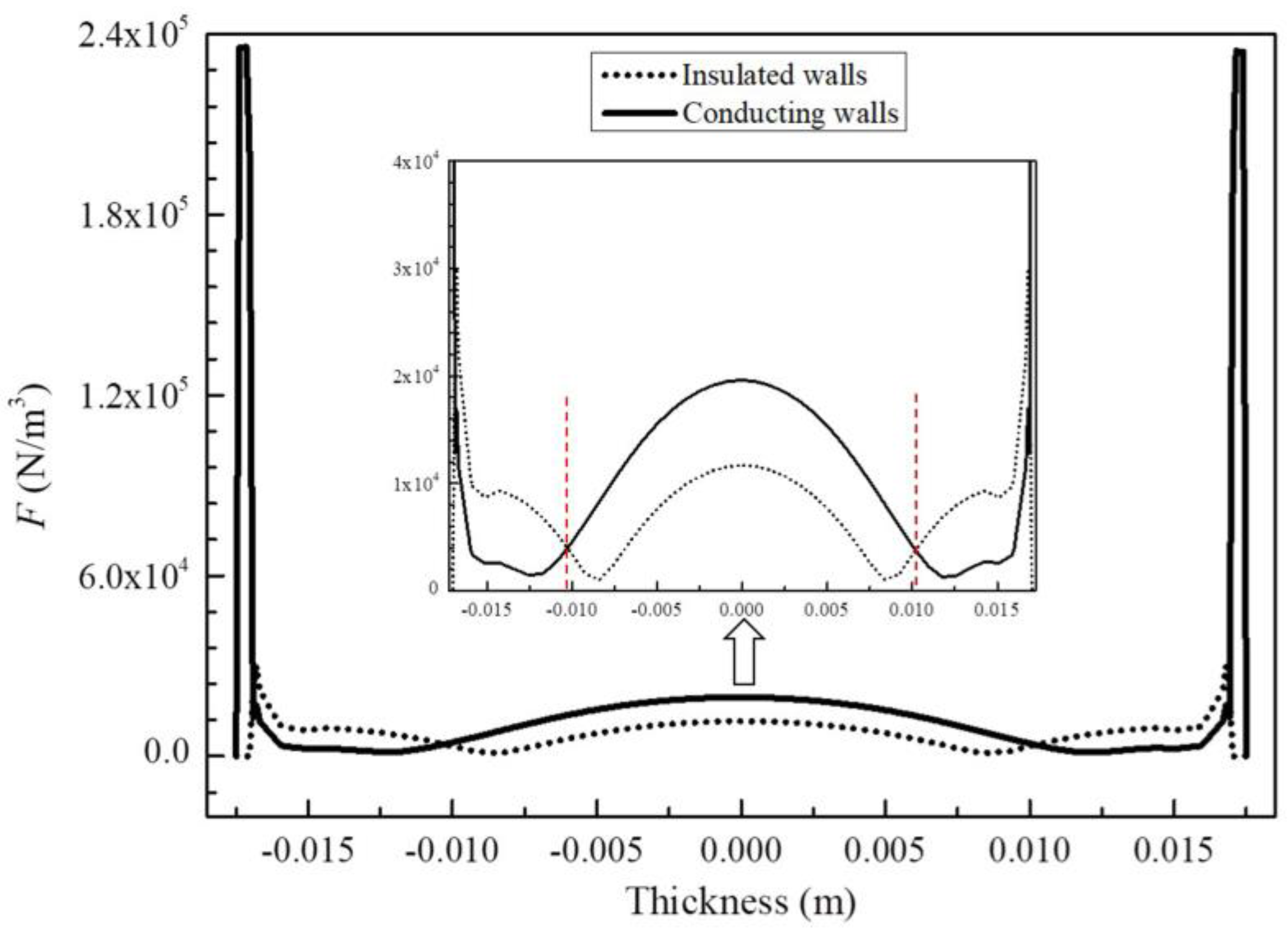
The influence of different conductive boundary conditions on the electromagnetic field was studied. Electrically-conducting walls can dramatically increase the density of the induced electrical current and electromagnetic force, and can have a stabilizing effect on the MHD turbulent flow. This conclusion indicates that in order to design EMBr for real CC processes, the consideration of the growing solid shell of steel is of crucial importance.

References

1. Grill, A.; Sorimachi, K.; Brimacombe, J.K. Heat flow, gap formation and break-outs in the continuous casting of steel slabs. Metall. Trans. B 1976, 7, 177–189. [Google Scholar] [CrossRef]
2. Guthrie, R.L. A review of fluid flows in liquid metal processing and casting operations. ISIJ Int. 2009, 49, 1453–1467. [Google Scholar] [CrossRef]
3. Lee, P.D.; Ramirez-Lopez, P.E.; Mills, K.C.; Santillana, B. Review: the “butterfly effect” in continuous casting. Ironmak. Steelmak. 2012, 39, 244–253. [Google Scholar] [CrossRef]
4. Thomas, B.G. Review on modeling and simulation of continuous casting. Steel Res. Int. 2018, 89, 1700312. [Google Scholar] [CrossRef]
5. Liu, Z.Q.; Li, B.K.; Zhang, L.; Xu, G.D. Analysis of transient transport and entrapment of particle in continuous casting mold. ISIJ Int. 2014, 54, 2324–2333. [Google Scholar] [CrossRef]
6. Liu, Z.Q.; Li, B.K.; Qi, F.S.; Cheung, S.C.P. Population balance modeling of polydispersed bubbly flow in continuous casting using average bubble number density approach. Powder Technol. 2017, 319, 139–147. [Google Scholar] [CrossRef]
7. Kim, D.; Kim, W.; Cho, K. Numerical simulation of the coupled turbulent flow and macroscopic solidification in continuous casting with electromagnetic brake. ISIJ Int. 2000, 40, 670–676. [Google Scholar] [CrossRef]
8. Harada, H.; Toh, T.; Ishii, T.; Kaneko, K.; Takeuchi, E. Effect of magnetic field conditions on the electromagnetic braking efficiency. ISIJ Int. 2001, 41, 1236–1244. [Google Scholar] [CrossRef]
9. Wang, Y.F.; Zhang, L.F. Fluid flow-related transport phenomena in steel slab continuous casting strands under electromagnetic brake. Metall. Mater. Trans. B 2011, 42, 1319–1351. [Google Scholar] [CrossRef]
10. Kubo, N.; Kubota, J.; Suzuki, M.; Ishii, T. Molten steel flow control under electromagnetic level accelerator in continuous casting mold. ISIJ Int. 2007, 47, 988–995. [Google Scholar] [CrossRef]
11. Timmel, K.; Eckert, S.; Gerbeth, G. Experimental investigation of the flow in a continuous casting mold under the influence of a transverse, direct current magnetic field. Metall. Mater. Trans. B 2011, 42, 68–80. [Google Scholar] [CrossRef]
12. Singh, R.; Thomas, B.G.; Vanka, S.P. Effect of a magnetic field on turbulent flow in the mold region of a steel caster. Metall. Mater. Trans. B 2013, 44, 1201–1221. [Google Scholar] [CrossRef]
13. Kratzsch, C.; Asad, A.; Schwarze, R. CFD of the MHD mold flow by means of hybrid LES/RANS turbulence modeling. J. Manuf. Sci. Prod. 2015, 15, 49–57. [Google Scholar] [CrossRef]
14. Thomas, B.G.; Singh, R.; Vanka, S.P.; Timmel, K.; Eckert, S.; Gerbeth, G. Effect of single-ruler electromagnetic braking (EMBr) location on transient flow in continuous casting. J. Manuf. Sci. Prod. 2015, 15, 93–104. [Google Scholar] [CrossRef]
15. Cho, S.M.; Kim, S.H.; Thomas, B.G. Transient fluid flow during steady continuous casting of steel slabs: part II. Effect of double-ruler electro-magnetic braking. ISIJ Int. 2014, 54, 855–864. [Google Scholar] [CrossRef]
16. Liu, Z.Q.; Li, L.M.; Li, B.K. Large eddy simulation of transient flow and inclusions transport in continuous casting mold under different electromagnetic brakes. JOM 2016, 68, 2180–2190. [Google Scholar] [CrossRef]
17. Li, B.K.; Okane, T.; Umeda, T. Modeling of molten metal flow in a continuous casting process considering the effects of argon gas injection and static magnetic-field application. Metall. Mater. Trans. B 2000, 31, 1491–1503. [Google Scholar] [CrossRef]
18. Miki, Y.; Takeuchi, S. Internal defects of continuous casting slabs caused by asymmetric unbalanced steel flow in mold. ISIJ Int. 2003, 43, 1548–1555. [Google Scholar] [CrossRef]
19. Zhang, Z.Q.; Yu, J.B.; Ren, Z.M.; Deng, K. Study on the liquid metal flow field in FC-mold of slab continuous casting. Adv. Manuf. 2015, 3, 212–220. [Google Scholar] [CrossRef]
20. Stefani, F.; Eckert, S.; Ratajczak, M.; Timmel, K.; Wondrak, T. Contactless inductive flow tomography: basic principles and first applications in the experimental modeling of continuous casting. IOP Conf. Ser. Mater. Sci. Eng. 2016, 143, 012023. [Google Scholar] [CrossRef]
21. Timmel, K.; Kratzsch, C.; Asad, A.; Schurmann, D.; Schwarze, S.; Eckert, S. Experimental and Numerical Modeling of Fluid Flow Processes in Continuous Casting: Results from the LIMMCAST-Project. IOP Conf. Ser. Mater. Sci. Eng. 2017, 228, 012019. [Google Scholar] [CrossRef] [Green Version]
22. Miao, X.C.; Timmel, K.; Lucas, D.; Ren, Z.M.; Eckert, S.; Gerbeth, G. Effect of an electromagnetic brake on the turbulent melt flow in a continuous casting mold. Metall. Mater. Trans. B 2012, 43, 954–972. [Google Scholar] [CrossRef]
23. Li, Z.; Wang, E.G.; Zhang, L.T.; Xu, Y.; Deng, A.Y. Influence of vertical electromagnetic brake on the steel/slag interface behavior in a slab mold. Metall. Mater. Trans. B 2017, 48, 2389–2402. [Google Scholar] [CrossRef]
24. Jin, K.; Vanka, S.P.; Thomas, B.G. Large eddy simulations of electromagnetic braking effects on argon bubble transport and capture in a steel continuous casting mold. Metall. Mater. Trans. B 2018, 49, 1360–1377. [Google Scholar] [CrossRef]
25. Vakhrushev, A.; Liu, Z.Q.; Wu, M.H.; Kharicha, A.; Ludwig, A.; Nitzl, G.; Tang, T.; Hackl, G. Numerical modeling of the MHD flow in continuous casting mold by two CFD platforms ANSYS Fluent and OpenFOAM. In Proceedings of the 7th International Congress on Science and Technology of Steelmaking, Venice, Italy, 13–15 June 2018. [Google Scholar]
26. Kharicha, A.; Alemany, A.; Bornas, D. Hydrodynamic study of a rotating MHD flow in a cylindrical cavity by ultrasound doppler shift method. Int. J. Eng. Sci. 2005, 43, 589–615. [Google Scholar] [CrossRef]
27. Kharicha, A.; Alemany, A.; Bornas, D. Influence of the magnetic field and the conductance ratio on the mass transfer in a lid driven flow. Int. J. Heat Mass Transf. 2004, 47, 1997–2014. [Google Scholar] [CrossRef]
28. Deloffre, P.; Terlain, A.; Alemany, A.; Kharicha, A. Corrosion study of an austenitic steel in Pb–17Li under magnetic field and rotating flow. Fusion Eng. Design 2003, 69, 391–395. [Google Scholar] [CrossRef]
29. Smagorinsky, J. General circulation experiments with the primitive equations. Month. Weather Rev. 1963, 91, 99–165. [Google Scholar] [CrossRef]
30. Chaudhary, R.; Ji, C.; Thomas, B.G.; Vanka, S.P. Transient turbulent flow in a liquid-metal model of continuous casting, including comparison of six different methods. Metall. Mater. Trans. B 2011, 42, 987–1007. [Google Scholar] [CrossRef]
31. Hunt, J.C.R.; Wray, A.A.; Moin, P. Eddies, stream, and convergence zones in turbulent flows. In Studying Turbulence Using Numerical Simulation Databases; Center for Turbulence Research Report N89; Center for Turbulence Research: Stanford, CA, USA, 1988; pp. 193–208. [Google Scholar]
Figure 1. Applied magnetic field profile in vertical direction [14]: (a) profile; (b) contour plot.
Metals 08 00609 g001
Figure 2. Computational domain and boundary conditions.
Metals 08 00609 g002
Figure 3. Transient horizontal velocity history at point 1 in the mold.
Metals 08 00609 g003
Figure 4. Time-averaged horizontal velocity profiles on three different lines across the mold.
Metals 08 00609 g004
Figure 5. Instantaneous iso-surfaces of Q-criterion (500 1/s2): (a) No EMBr (electromagnetic brake); (b) EMBr with electrically-insulated walls; (c) EMBr with electrically-conducting walls.
Metals 08 00609 g005
Figure 6. Instantaneous iso-surfaces of Q-criterion for the case applying EMBr with electrically-insulated walls at: (a) 14 s; (b) 16 s; (c) 18 s; (d) 20 s.
Metals 08 00609 g006
Figure 7. Transient horizontal velocity history at point 1 (Figure 2).
Metals 08 00609 g007
Figure 8. Instantaneous iso-surfaces of the Q-criterion for the case applying EMBr with electrically-conducting walls at: (a) 14 s; (b) 16 s; (c) 18 s; (d) 20 s.
Metals 08 00609 g008
Figure 9. Contours of time-averaged velocity: (a) No EMBr; (b) EMBr with electrically-insulated walls; (c) EMBr with electrically-conducting walls.
Metals 08 00609 g009
Figure 10. Contours of time-averaged induced electrical current density on plane 1 (Figure 2) for: (a) EMBr with electrically-insulated walls; (b) EMBr with electrically-conducting walls.
Metals 08 00609 g010
Figure 11. Time-averaged induced electrical current density distribution on line 4 (refer to Figure 10).
Metals 08 00609 g011
Figure 12. Vectors of time-averaged induced electrical current on plane 1 (a) EMBr with electrically-insulated walls; (b) EMBr with electrically-conducting walls.
Metals 08 00609 g012
Figure 13. Contours of time-averaged electromagnetic force on plane 1 (a) EMBr with electrically-insulated walls; (b) EMBr with electrically-conducting walls.
Metals 08 00609 g013
Figure 14. Time-averaged electromagnetic force distribution on line 4.
Metals 08 00609 g014