
A Buckling Instability Prediction Model for the Reliable Design of Sheet Metal Panels Based on an Artificial Intelligent Self-Learning Algorithm


Abstract
:1. Introduction
- The buckling instability of sheet metal panels can be estimated in the early design stages based on the modeling curvatures, avoiding expensive and time-consuming redesigns of the forming die;
- Both experimental and finite element results can be included in the training and validation data sets, allowing extension of the range of validity and applicability of the developed algorithm;
- The implemented image-based CNN methodology proved that machine learning algorithms can also already be utilized for optimization during the early stages of the design process. Moreover, although the methodology proposed in this paper was applied to sheet metal panels for the prediction of the buckling instability, it can be extended to different processes by accounting for the desired target function by applying the same implementation procedure presented in this paper.
2. Numerical Model Implementation
3. Curvature Calculation Procedure
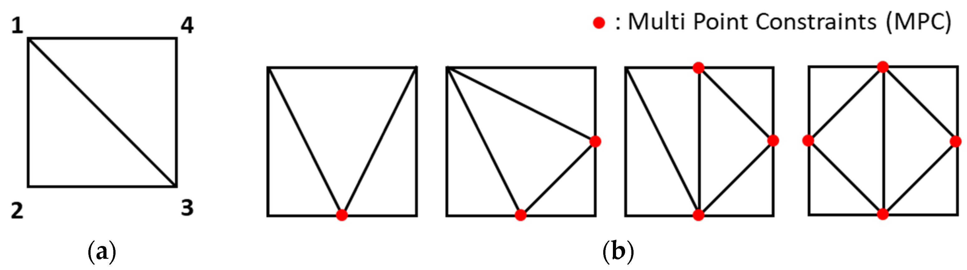
3.1. Quadrilateral Mesh into Triangular Mesh Conversion
3.2. Vertex Normal Vector Calculation
3.3. Nodal Curvature Calculation
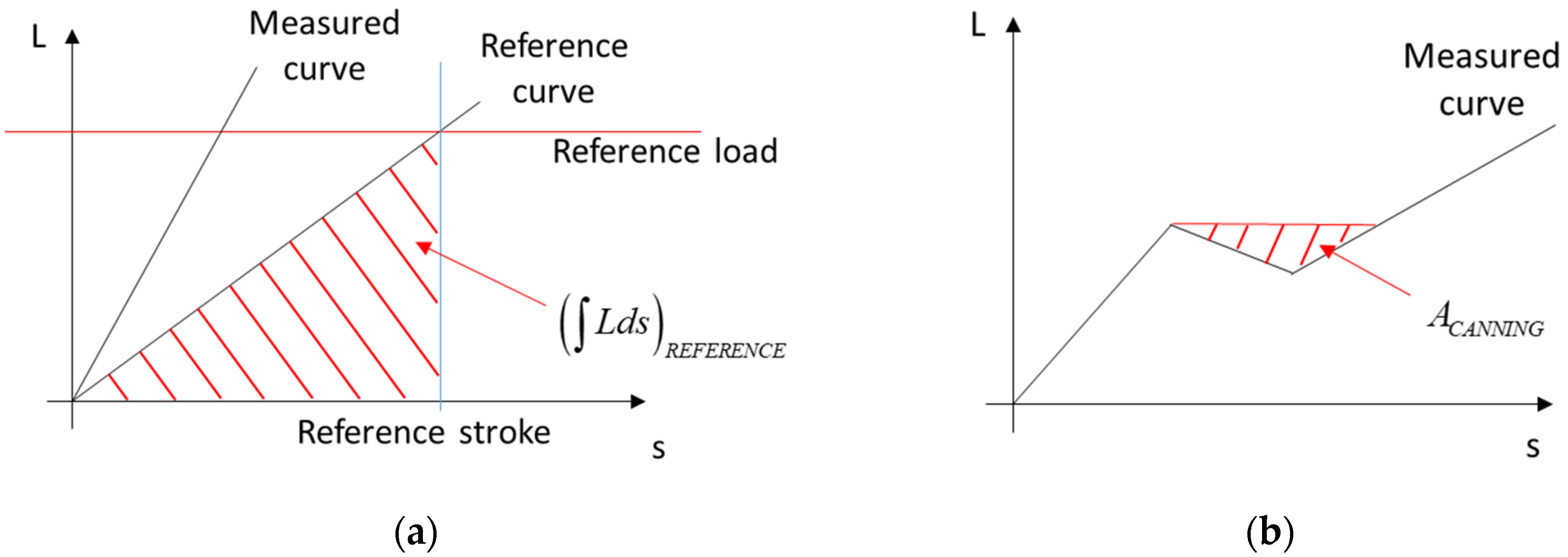
4. Buckling Instability Definition and Calculation
5. CNN Deep-Learning Algorithm Development and Training
5.1. Neural Network (NN) Model Development
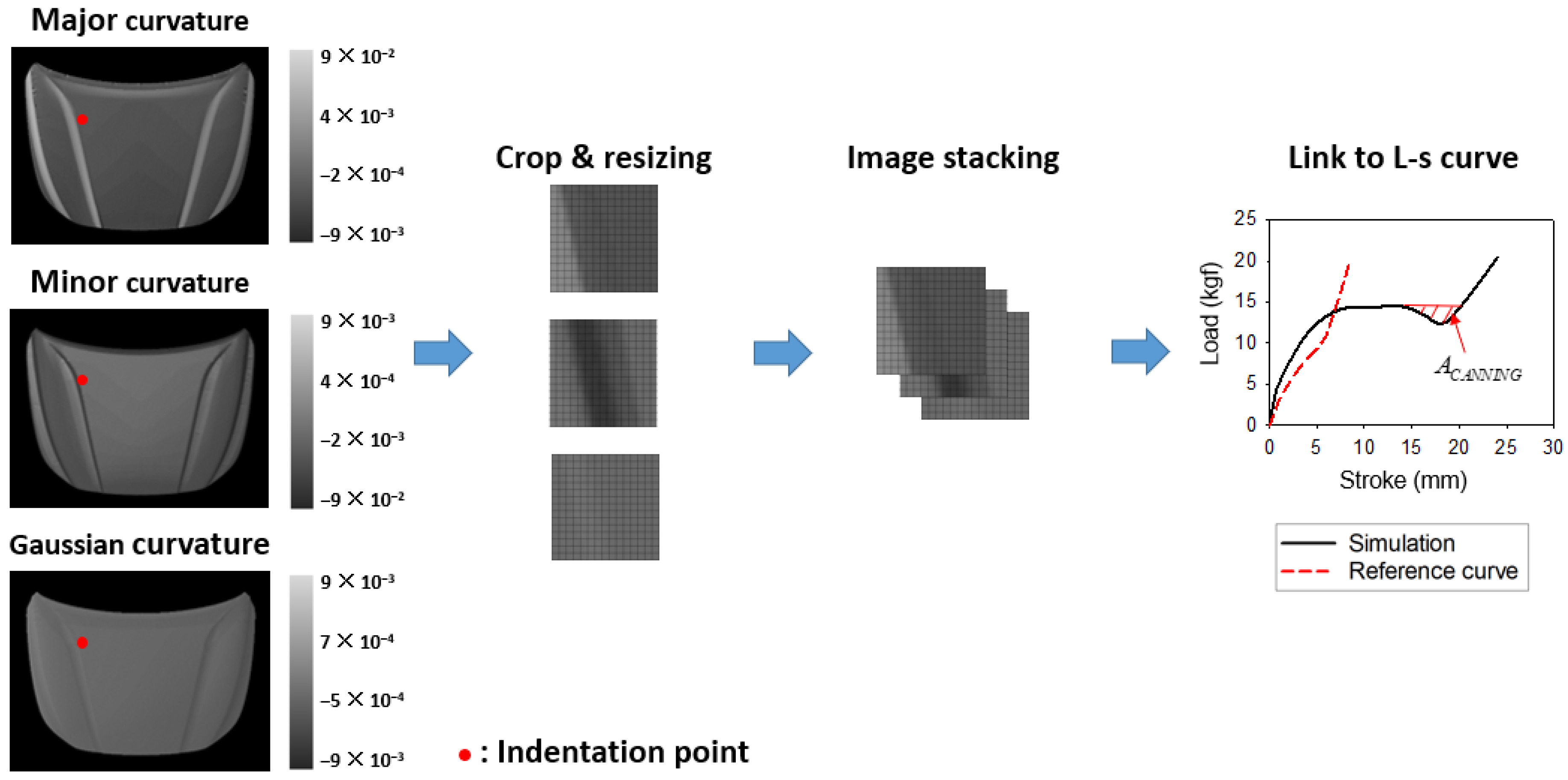
5.2. Pre-Processing
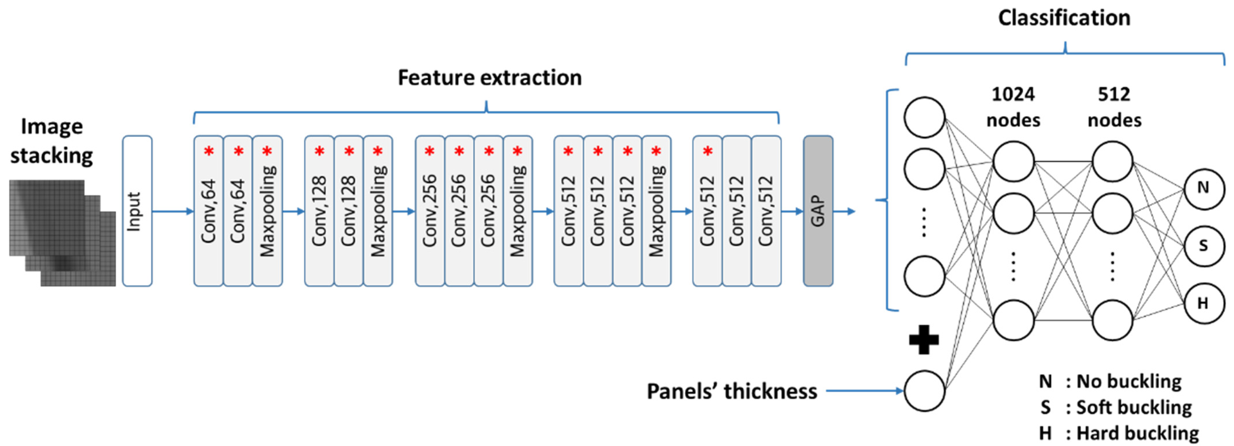
5.3. CNN Model Structure, Training, and Cross-Validation
6. Denting Resistance Validation Experiments
7. Results
8. Discussion
9. Conclusions
Author Contributions
Funding
Institutional Review Board Statement
Informed Consent Statement
Data Availability Statement
Acknowledgments
Conflicts of Interest
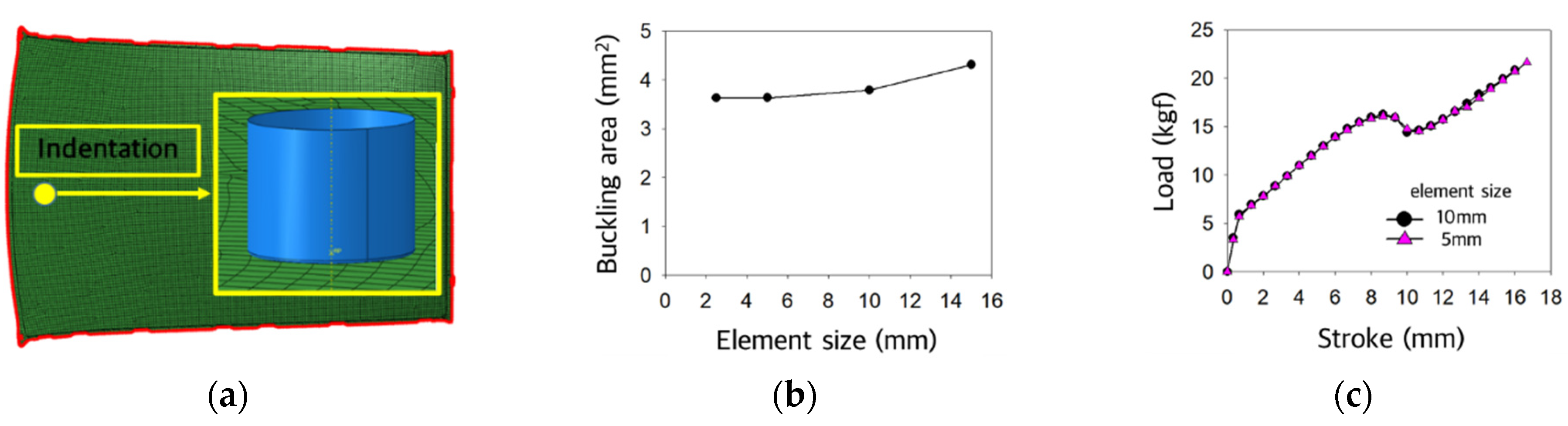
Appendix A. The Mesh Sensitivity for Roof Panels (h-Convergence)

Appendix B. The Detailed Dimensions and Canning Results for Considered Panels

| Model | P# | x | y | z | Maj.Curv. | Min.Curv. | Gauss.Curv. | RES |
|---|---|---|---|---|---|---|---|---|
| M#3 Fender | #1 | 650 | 100 | 30 | −1.80 × 10⁻⁴ | 1.23 × 10⁻³ | −2.23 × 10⁻⁷ | N |
| #2 | 550 | 0 | 68 | 1.76 × 10⁻⁴ | 1.66 × 10⁻³ | 2.91 × 10⁻⁷ | N | |
| #3 | 650 | −50 | 70 | 1.37 × 10⁻⁴ | 1.20 × 10⁻³ | 1.65 × 10⁻⁷ | N | |
| M#1 Front Door | #1 | 370 | −265 | 135 | −1.19 × 10⁻³ | −1.37 × 10⁻⁵ | 1.64 × 10⁻⁸ | N |
| #2 | 485 | −97 | 105 | −2.56 × 10⁻⁵ | 1.65 × 10⁻³ | −4.21 × 10⁻⁸ | S | |
| #3 | 795 | −95 | 105 | −3.59 × 10⁻⁵ | 7.26 × 10⁻⁴ | −2.60 × 10⁻⁸ | H | |
| M#2 Roof | #1 | 500 | 0 | 112 | −9.08 × 10⁻³ | −2.90 × 10⁻⁴ | 2.63 × 10⁻⁶ | N |
| #2 | 465 | 320 | 108 | −9.65 × 10⁻³ | −5.03 × 10⁻⁵ | 4.85 × 10⁻⁷ | S | |
| #3 | 600 | 320 | 119 | −8.60 × 10⁻³ | −5.38 × 10⁻⁵ | 4.62 × 10⁻⁷ | H | |
| M#4 Rear Door | #1 | 240 | −200 | 105 | −1.81 × 10⁻³ | −1.62 × 10⁻⁵ | 2.92 × 10⁻⁸ | N |
| #2 | 860 | −230 | 100 | −9.16 × 10⁻⁴ | 2.56 × 10⁻⁵ | −2.35 × 10⁻⁸ | N | |
| #3 | 450 | −450 | 103 | −5.69 × 10⁻⁴ | 1.86 × 10⁻⁴ | −1.06 × 10⁻⁷ | N | |
| M#3 Hood | #1 | 450 | 750 | 245 | −2.49 × 10⁻⁴ | −8.62 × 10⁻⁵ | 2.15 × 10⁻⁸ | N |
| #2 | −200 | 700 | 251 | −1.90 × 10⁻⁴ | −1.14 × 10⁻⁴ | 2.17 × 10⁻⁸ | H | |
| #3 | 0 | 450 | 210 | −2.29 × 10⁻⁴ | −1.96 × 10⁻⁴ | 4.50 × 10⁻⁸ | H | |
| M#5 Door | #1 | 130 | −130 | 88 | −1.78 × 10⁻³ | −3.64 × 10⁻⁵ | 6.46 × 10⁻⁸ | N |
| #2 | 350 | −80 | 74 | −4.43 × 10⁻² | 4.67 × 10⁻⁵ | −2.07 × 10⁻⁶ | N | |
| #3 | 550 | −120 | 80 | 1.61 × 10⁻⁵ | 8.40 × 10⁻³ | 1.35 × 10⁻⁷ | N | |
| #4 | 220 | −190 | 100 | −3.87 × 10⁻³ | −2.48 × 10⁻⁵ | 9.60 × 10⁻⁸ | H | |
| #5 | 350 | −200 | 100 | −3.05 × 10⁻³ | 4.51 × 10⁻⁵ | −1.38 × 10⁻⁷ | N | |
| #6 | 470 | −210 | 100 | −1.51 × 10⁻³ | 1.20 × 10⁻⁴ | −1.80 × 10⁻⁷ | N | |
| #7 | 580 | −240 | 104 | −1.61 × 10⁻³ | 1.56 × 10⁻⁴ | −2.51 × 10⁻⁷ | N | |
| #8 | 680 | −200 | 99 | −1.81 × 10⁻³ | 1.05 × 10⁻⁴ | −1.90 × 10⁻⁷ | N | |
| #9 | 130 | −330 | 104 | −9.75 × 10⁻⁴ | 2.23 × 10⁻⁵ | −2.17 × 10⁻⁸ | N | |
| #10 | 290 | −330 | 103 | −9.41 × 10⁻⁴ | 1.20 × 10⁻⁴ | −1.13 × 10⁻⁷ | N | |
| #11 | 450 | −330 | 105 | −7.78 × 10⁻⁴ | 2.56 × 10⁻⁴ | −2.00 × 10⁻⁷ | N | |
| #12 | 590 | −330 | 110 | −6.26 × 10⁻⁴ | 2.87 × 10⁻⁴ | −1.80 × 10⁻⁷ | N | |
| #13 | 210 | −420 | 100 | −6.80 × 10⁻⁴ | 1.44 × 10⁻⁴ | −9.82 × 10⁻⁸ | N | |
| #14 | 370 | −420 | 100 | −5.59 × 10⁻⁴ | 4.75 × 10⁻⁴ | −2.65 × 10⁻⁷ | N | |
| #15 | 530 | −420 | 107 | −4.29 × 10⁻⁴ | 5.25 × 10⁻⁴ | −2.25 × 10⁻⁷ | N | |
| #16 | 130 | −510 | 88 | 1.30 × 10⁻⁴ | 1.65 × 10⁻³ | 2.13 × 10⁻⁷ | N | |
| #17 | 290 | −510 | 88 | −3.96 × 10⁻⁴ | 6.17 × 10⁻⁴ | −2.44 × 10⁻⁷ | N | |
| #18 | 450 | −510 | 98 | −6.66 × 10⁻⁴ | 8.57 × 10⁻⁴ | −5.71 × 10⁻⁷ | N | |
| #19 | 460 | −35 | 55 | −3.16 × 10⁻³ | 5.37 × 10⁻⁵ | −1.70 × 10⁻⁷ | N | |
| #20 | 595 | −10 | 42 | −2.26 × 10⁻⁵ | 8.93 × 10⁻³ | −2.02 × 10⁻⁷ | N | |
| #21 | 750 | −20 | 25 | −3.57 × 10⁻⁴ | 9.15 × 10⁻³ | −3.26 × 10⁻⁶ | N | |
| #22 | 875 | −20 | 54 | −6.11 × 10⁻³ | −2.66 × 10⁻⁴ | 1.63 × 10⁻⁶ | N |
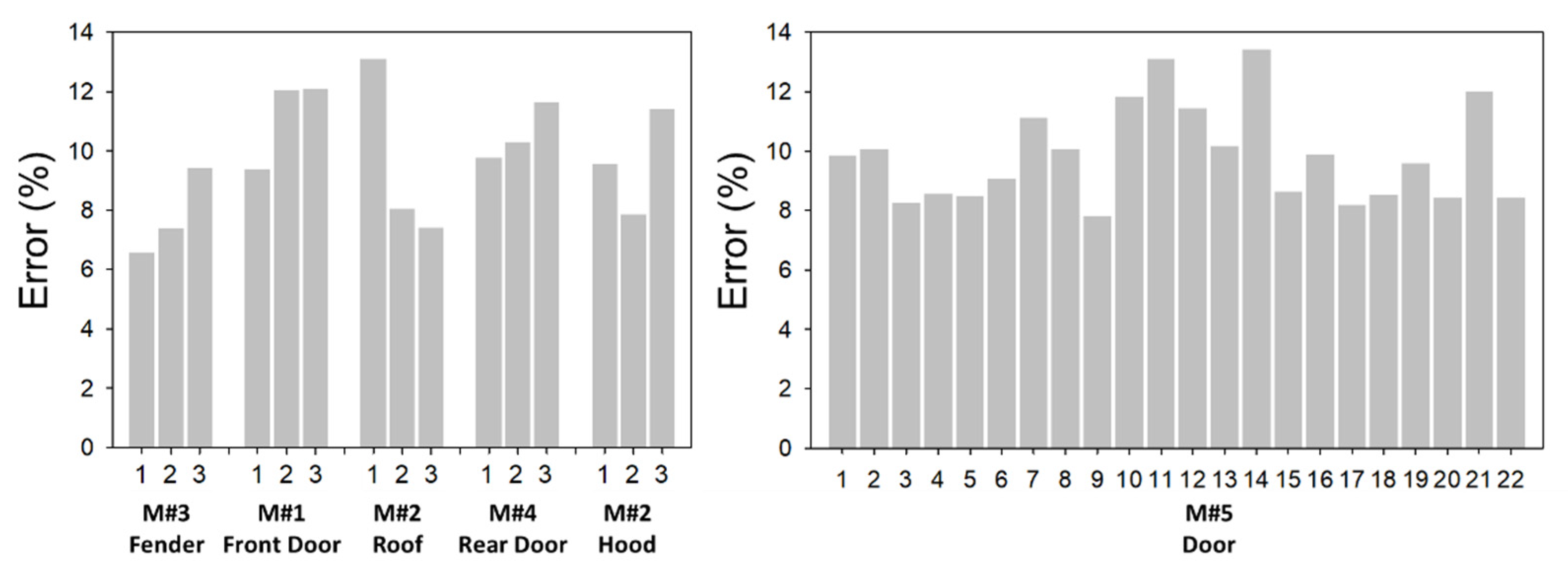
| Model | P# | EXP. Area (mm2) | FEA Area (mm2) | Error (%) | AR | Model | P# | EXP. Area (mm2) | FEA Area (mm2) | Error (%) | AR |
|---|---|---|---|---|---|---|---|---|---|---|---|
| M#3 Fender | #1 | 44.45 | 47.38 | 6.59 | 0 | M#5 Door | #5 | 158.65 | 172.12 | 8.49 | 0 |
| #2 | 21.26 | 22.83 | 7.40 | 0 | #6 | 131.62 | 143.57 | 9.08 | 0 | ||
| #3 | 50.01 | 54.72 | 9.43 | 0 | #7 | 84.09 | 93.45 | 11.13 | 0 | ||
| M#1 Front Door | #1 | 49.95 | 54.65 | 9.40 | 0 | #8 | 80.75 | 72.60 | 10.09 | 0 | |
| #2 | 79.94 | 89.57 | 12.05 | 0.07 | #9 | 96.79 | 89.22 | 7.82 | 0 | ||
| #3 | 72.49 | 81.27 | 12.11 | 2.59 | #10 | 77.05 | 86.17 | 11.84 | 0 | ||
| M#2 Roof | #1 | 313.01 | 354.07 | 13.12 | 0 | #11 | 101.89 | 115.26 | 13.12 | 0 | |
| #2 | 229.83 | 248.36 | 8.06 | 0.54 | #12 | 121.12 | 107.23 | 11.47 | 0 | ||
| #3 | 204.45 | 219.63 | 7.43 | 2.52 | #13 | 76.76 | 68.94 | 10.18 | 0 | ||
| M#4 Rear Door | #1 | 94.43 | 103.66 | 9.77 | 0 | #14 | 222.01 | 192.16 | 13.44 | 0 | |
| #2 | 100.60 | 90.23 | 10.31 | 0 | #15 | 326.91 | 355.21 | 8.66 | 0 | ||
| #3 | 97.51 | 86.13 | 11.67 | 0 | #16 | 99.85 | 109.74 | 9.91 | 0 | ||
| M#3 Hood | #1 | 132.75 | 145.46 | 9.58 | 0 | #17 | 265.83 | 244.01 | 8.21 | 0 | |
| #2 | 244.89 | 264.16 | 7.87 | 15.95 | #18 | 376.46 | 344.23 | 8.56 | 0 | ||
| #3 | 340.96 | 379.95 | 11.44 | 2.89 | #19 | 328.76 | 360.36 | 9.61 | 0 | ||
| M#5 Door | #1 | 72.19 | 79.31 | 9.87 | 0 | #20 | 370.89 | 402.18 | 8.44 | 0 | |
| #2 | 177.16 | 159.32 | 10.07 | 0 | #21 | 268.97 | 301.27 | 12.01 | 0 | ||
| #3 | 135.57 | 124.34 | 8.29 | 0 | #22 | 312.28 | 285.94 | 8.43 | 0 | ||
| #4 | 144.81 | 132.39 | 8.58 | 3.09 |
| Model | P# | x | y | z | Maj. Curv. | Min. Curv. | Gauss. Curv. | Pred. Res. | FEA Res. |
|---|---|---|---|---|---|---|---|---|---|
| M#1 Hood | #1 | 750 | 450 | 177 | −9.90 × 10⁻³ | −2.16 × 10⁻⁵ | 2.14 × 10⁻⁷ | S | S |
| #2 | 700 | −200 | 187 | −2.17 × 10⁻⁴ | −1.09 × 10⁻⁴ | 2.36 × 10⁻⁸ | H | H | |
| #3 | 450 | 0 | 466 | −2.60 × 10⁻⁴ | −2.54 × 10⁻⁴ | 6.62 × 10⁻⁸ | H | H | |
| #4 | 250 | −600 | 43 | −5.60 × 10⁻⁴ | 3.79 × 10⁻³ | −2.12 × 10⁻⁶ | N | N | |
| #5 | 550 | 650 | 121 | −2.38 × 10⁻³ | −3.16 × 10⁻⁴ | 7.53 × 10⁻⁷ | H | H | |
| #6 | 700 | −700 | 137 | −1.00 × 10⁻² | −2.63 × 10⁻⁴ | 2.64 × 10⁻⁶ | H | H | |
| #7 | 850 | 750 | 137 | −3.76 × 10⁻⁴ | 4.88 × 10⁻³ | −1.84 × 10⁻⁶ | S | N | |
| #8 | 250 | −450 | 68 | −1.03 × 10⁻³ | −3.32 × 10⁻⁴ | 3.43 × 10⁻⁷ | N | N | |
| #9 | 450 | 550 | 112 | −1.09 × 10⁻³ | −3.53 × 10⁻⁴ | 3.84 × 10⁻⁷ | H | H | |
| #10 | 450 | −450 | 114 | −7.45 × 10⁻⁴ | −2.72 × 10⁻⁴ | 2.02 × 10⁻⁷ | S | S | |
| #11 | 650 | 500 | 146 | −6.96 × 10⁻⁴ | −2.25 × 10⁻⁴ | 1.56 × 10⁻⁷ | N | N | |
| #12 | 900 | −550 | 175 | −1.02 × 10⁻⁴ | 5.83 × 10⁻⁴ | −5.96 × 10⁻⁸ | H | H | |
| #13 | 250 | 350 | 73 | −4.68 × 10⁻⁴ | 8.77 × 10⁻³ | −4.10 × 10⁻⁶ | N | S | |
| #14 | 600 | −400 | 148 | −1.43 × 10⁻² | −2.29 × 10⁻⁴ | 3.27 × 10⁻⁶ | N | N | |
| #15 | 200 | −200 | 82 | −6.59 × 10⁻⁴ | −3.66 × 10⁻⁴ | 2.41 × 10⁻⁷ | H | H | |
| #16 | 500 | 200 | 147 | −3.60 × 10⁻⁴ | −1.95 × 10⁻⁴ | 7.02 × 10⁻⁸ | N | N | |
| #17 | 250 | 0 | 102 | −5.83 × 10⁻⁴ | −3.80 × 10⁻⁴ | 2.22 × 10⁻⁷ | H | H | |
| #18 | 850 | 0 | 466 | −1.52 × 10⁻⁴ | −1.35 × 10⁻⁴ | 2.05 × 10⁻⁸ | N | N |
References
- Jung, D.W. A parametric study of sheet metal denting using a simplified design approach. KSME Int. J. 2002, 16, 1673–1686. [Google Scholar] [CrossRef]
- Dicello, J.A.; George, R.A. Design criteria for the dent resistance of auto body panels. SAE Tech. Pap. 1974, 389–397. [Google Scholar] [CrossRef]
- Guo, M.; Hu, Y.; Sanghera, R. Finite Element Analyses and Correlations on Oil Canning of a Door Outer Panel; SAE Technical Paper; SAE International: Warrendale, PA, USA, 2009; pp. 1–6. [Google Scholar] [CrossRef]
- Johnson, T.E.; Schaffnit, W.O. Dent Resistance of Cold-Rolled Low-Carbon Steel Sheet; SAE Technical Paper; SAE International: Warrendale, PA, USA, 1973; Volume 82, pp. 1719–1730. [Google Scholar] [CrossRef]
- Lu, H.; Ma, M.; You, J.; Li, Z. Dent resistance for automobile body panels. Chin. J. Mech. Eng. 2009, 22, 903–911. [Google Scholar] [CrossRef]
- Shih, H.C.; Horvath, C.D. Effects of Material Bending and Hardening on Dynamic Dent Resistance; SAE Technical Paper; SAE International: Warrendale, PA, USA, 2005. [Google Scholar] [CrossRef]
- Holmberg, S.; Thilderkvist, P. Influence of material properties and stamping conditions on the stiffness and static dent resistance of automotive panels. Mater. Des. 2002, 23, 681–691. [Google Scholar] [CrossRef]
- Ekstrand, G.; Asnafi, N. On testing of the stiffness and the dent resistance of autobody panels. Mater. Des. 1998, 19, 145–156. [Google Scholar] [CrossRef]
- Asnafi, N. On strength, stiffness and dent resistance of car body panels. J. Mater. Process. Tech. 1995, 49, 13–31. [Google Scholar] [CrossRef]
- Holmberg, S.; Nejabat, B. Numerical assessment of stiffness and dent properties of automotive exterior panels. Mater. Des. 2004, 25, 361–368. [Google Scholar] [CrossRef]
- Shen, H.; Li, S.; Chen, G. Numerical analysis of panels’ dent resistance considering the Bauschinger effect. Mater. Des. 2010, 31, 870–876. [Google Scholar] [CrossRef]
- Shen, H.; Li, S.; Chen, G. Quantitative analysis of surface deflections in the automobile exterior panel based on a curvature-deviation method. J. Mater. Process. Technol. 2012, 212, 1548–1556. [Google Scholar] [CrossRef]
- Park, C.D.; Chung, W.J.; Kim, B.M. A numerical and experimental study of surface deflections in automobile exterior panels. J. Mater. Process. Technol. 2007, 187–188, 99–102. [Google Scholar] [CrossRef]
- Soltoggio, A.; Stanley, K.O.; Risi, S. Born to learn: The inspiration, progress, and future of evolved plastic artificial neural networks. Neural Netw. 2018, 108, 48–67. [Google Scholar] [CrossRef] [Green Version]
- Patel, H.V.; Panda, A.; Kuipers, J.A.M.; Peters, E.A.J.F. Computing interface curvature from volume fractions: A machine learning approach. Comput. Fluids 2019, 193, 104263. [Google Scholar] [CrossRef]
- Yusri, I.M.; Abdul Majeed, A.P.P.; Mamat, R.; Ghazali, M.F.; Awad, O.I.; Azmi, W.H. A review on the application of response surface method and artificial neural network in engine performance and exhaust emissions characteristics in alternative fuel. Renew. Sustain. Energy Rev. 2018, 90, 665–686. [Google Scholar] [CrossRef]
- Schmidhuber, J. Deep Learning in neural networks: An overview. Neural Netw. 2015, 61, 85–117. [Google Scholar] [CrossRef] [PubMed] [Green Version]
- Winiczenko, R. Effect of friction welding parameters on the tensile strength and microstructural properties of dissimilar AISI 1020-ASTM A536 joints. Int. J. Adv. Manuf. Technol. 2016. [Google Scholar] [CrossRef] [Green Version]
- Mirandola, I.; Berti, G.A.; Caracciolo, R.; Lee, S.; Kim, N.; Quagliato, L. Machine learning-based models for the estimation of the energy consumption in metal forming processes. Metals 2021, 11, 833. [Google Scholar] [CrossRef]
- Feng, S.; Zhou, H.; Dong, H. Using deep neural network with small dataset to predict material defects. Mater. Des. 2019, 162, 300–310. [Google Scholar] [CrossRef]
- Kim, H.; Al-Saeedi, S.; Jang, C.; Quagliato, L.; Kim, N. Development of an index model for oil canning of steel sheet metal forming products. Int. J. Adv. Manuf. Technol. 2018. [Google Scholar] [CrossRef]
- Max, N. Weights for Computing Vertex Normals from Facet Normals. Graph. Tools—Jgt Ed. Choice 2005, 75–81. [Google Scholar] [CrossRef]
- Rusinkiewicz, S. Estimating curvatures and their derivatives on triangle meshes. In Proceedings of the Second International Symposium on 3D Data Processing, Visualization, and Transmission: 3DPVT 2004, Thessaloniki, Greece, 6–9 September 2004; pp. 486–493. [Google Scholar] [CrossRef]
- Rumelhart, D.E.; Hinton, G.E.; Williams, R.J. Learning representations by back-propagating errors. Nature 1986, 323, 533–536. [Google Scholar] [CrossRef]
- Cherry, J.M.; Adler, C.; Ball, C.; Chervitz, S.A.; Dwight, S.S.; Hester, E.T.; Jia, Y.; Juvik, G.; Roe, T.; Schroeder, M.; et al. SGD: Saccharomyces genome database. Nucleic Acids Res. 1998, 26, 73–79. [Google Scholar] [CrossRef]
- Kingma, D.P.; Ba, J.L. Adam: A method for stochastic optimization. In Proceedings of the 3rd International Conference on Learning Representations, ICLR 2015, San Diego, CA, USA, 7–9 May 2015; pp. 1–15. [Google Scholar]
- Krizhevsky, A.; Sutskever, I.; Hinton, G.E. ImageNet classification with deep convolutional neural networks. Adv. Neural Inf. Process. Syst. 2012, 2, 1097–1105. [Google Scholar] [CrossRef]
- Simonyan, K.; Zisserman, A. Very deep convolutional networks for large-scale image recognition. In Proceedings of the 3rd International Conference on Learning Representations, ICLR 2015, San Diego, CA, USA, 7–9 May 2015; pp. 1–14. [Google Scholar]
- Yosinski, J.; Clune, J.; Bengio, Y.; Lipson, H. How transferable are features in deep neural networks? Adv. Neural Inf. Process. Syst. 2014, 4, 3320–3328. [Google Scholar]
- Vogado, L.H.S.; Veras, R.M.S.; Araujo, F.H.D.; Silva, R.R.V.; Aires, K.R.T. Leukemia diagnosis in blood slides using transfer learning in CNNs and SVM for classification. Eng. Appl. Artif. Intell. 2018, 72, 415–422. [Google Scholar] [CrossRef]
- Srivastava, N.; Hinton, G.; Krizhevsky, A.; Sutskever, I.; Salakhutdinov, R. Dropout: A simple way to prevent neural networks from overfitting. J. Mach. Learn. Res. 2014, 15, 1929–1958. [Google Scholar]


| n-Fold | 1 | 2 | 3 | 4 | 5 | Average |
|---|---|---|---|---|---|---|
| Accuracy | 0.908 | 0.886 | 0.899 | 0.914 | 0.897 | 0.901 |
| score | 0.909 | 0.898 | 0.900 | 0.921 | 0.907 | 0.907 |
| Panel Model | P# | Experiments | Proposed Model | Jung [1] | Kim et al. [30] | Panel Model | P# | Experiments | Proposed Model | Jung [1] | Kim et al. [30] |
|---|---|---|---|---|---|---|---|---|---|---|---|
| M#3 Fender | #1 | N | N | N | N | M#5 Door | #5 | N | N | N | N |
| #2 | N | N | N | N | #6 | N | N | N | N | ||
| #3 | N | N | N | N | #7 | N | N | N | N | ||
| M#1 Front Door | #1 | N | N | N | N | #8 | N | N | N | N | |
| #2 | S | S | N | N | #9 | N | N | N | N | ||
| #3 | H | H | N | N | #10 | N | N | N | N | ||
| M#2 Roof | #1 | N | N | N | N | #11 | N | N | N | N | |
| #2 | S | S | N | N | #12 | N | N | N | N | ||
| #3 | H | H | N | N | #13 | N | N | N | N | ||
| M#4 Rear Door | #1 | N | N | N | N | #14 | N | N | N | N | |
| #2 | N | N | N | N | #15 | N | N | N | N | ||
| #3 | N | N | N | N | #16 | N | N | N | N | ||
| M#3 Hood | #1 | N | N | N | N | #17 | N | N | N | N | |
| #2 | H | H | H | H | #18 | N | N | N | N | ||
| #3 | H | H | N | H | #19 | N | N | N | N | ||
| M#5 Door | #1 | N | N | N | N | #20 | N | N | N | N | |
| #2 | N | N | N | N | #21 | N | N | N | N | ||
| #3 | N | N | N | N | #22 | N | N | N | N | ||
| #4 | H | H | H | H |
Publisher’s Note: MDPI stays neutral with regard to jurisdictional claims in published maps and institutional affiliations. |
© 2021 by the authors. Licensee MDPI, Basel, Switzerland. This article is an open access article distributed under the terms and conditions of the Creative Commons Attribution (CC BY) license (https://creativecommons.org/licenses/by/4.0/).
Share and Cite
Lee, S.; Quagliato, L.; Park, D.; Berti, G.A.; Kim, N. A Buckling Instability Prediction Model for the Reliable Design of Sheet Metal Panels Based on an Artificial Intelligent Self-Learning Algorithm. Metals 2021, 11, 1533. https://doi.org/10.3390/met11101533
Lee S, Quagliato L, Park D, Berti GA, Kim N. A Buckling Instability Prediction Model for the Reliable Design of Sheet Metal Panels Based on an Artificial Intelligent Self-Learning Algorithm. Metals. 2021; 11(10):1533. https://doi.org/10.3390/met11101533
Chicago/Turabian StyleLee, Seungro, Luca Quagliato, Donghwi Park, Guido A. Berti, and Naksoo Kim. 2021. "A Buckling Instability Prediction Model for the Reliable Design of Sheet Metal Panels Based on an Artificial Intelligent Self-Learning Algorithm" Metals 11, no. 10: 1533. https://doi.org/10.3390/met11101533