Mathematical Models for Simulation and Optimization of High-Flux Solar Furnaces

Abstract

High-flux solar furnaces distributed throughout the world have been designed and constructed individually, i.e., on a one-by-one basis because there are several possible optical configurations that must take into account the geographical location and the maximum power to be attained. In this work, three ray-tracing models were developed to simulate the optical paths travelled by sun rays in solar furnaces of high concentration using as an example, the solar furnace SF60 of the Plataforma Solar de Almería, in Spain. All these simulation models are supported by mathematical constructions, which are also presented. The first model assumes a random distribution of sun rays coming from a concentrator with spherical curvature. The second model assumes that a random distribution of parallel rays coming from the heliostat is reflected by a concentrator with spherical curvature. Finally, the third model considers that the random parallel rays are reflected by a concentrator with a paraboloid curvature. The three models are all important in optical geometry, although the paraboloid model is more adequate to optimize solar furnaces. The models are illustrated by studying the influence of mirror positioning and shutter attenuation. Additionally, ray-tracing simulations confirmed the possibility to attain homogenous distribution of flux by means of double reflexion using two paraboloid surfaces.

1. Introduction

The simplest aspects of the interaction between light and matter have been known since at least the Classic Antiquity, including topics such as the reflexion and the refraction of light when it contacts a medium denser than air, such as water or a glass (according to legend, Archimedes may have used mirrors to defend Syracuse against the romans, circa 213–212 BC). The Snell-Descartes law, a cornerstone of geometrical optics, was successively discovered by Ibn Sahl, active in Baghdad during the 980s [1], Willebrord Snellius in circa 1621, and René Descartes in 1637 [2]. From 1011 to 1021, Ibn al-Haytham published a seven-volume treatise titled “The Book of Optics”. In 1704, Isaac Newton published his famous Opticks, “a treatise of the reflexions, refractions, inflexions and colours of light”, which was a result of experiments and the deductions made from them. At the beginning of the 19th century—with the works of Thomas Young [3] and Augustin-Jean Fresnel—light started to be understood as a wave phenomenon. The interferences and the diffraction of light could then be explained and Fresnel’s equations for reflection and refraction/transmission were derived. The polarization of light could be understood and the polarization of reflected and refracted light could be calculated, including the limit and Brewster angles, which are essential to understand optical fibres and lasers [4,5]. Nowadays, despite the decisive importance of physical optics, geometrical optics continues to play a fundamental role in the analysis and design of optical systems involving lenses, mirrors, and other devices in which the wave character of light does not need to be taken into account.

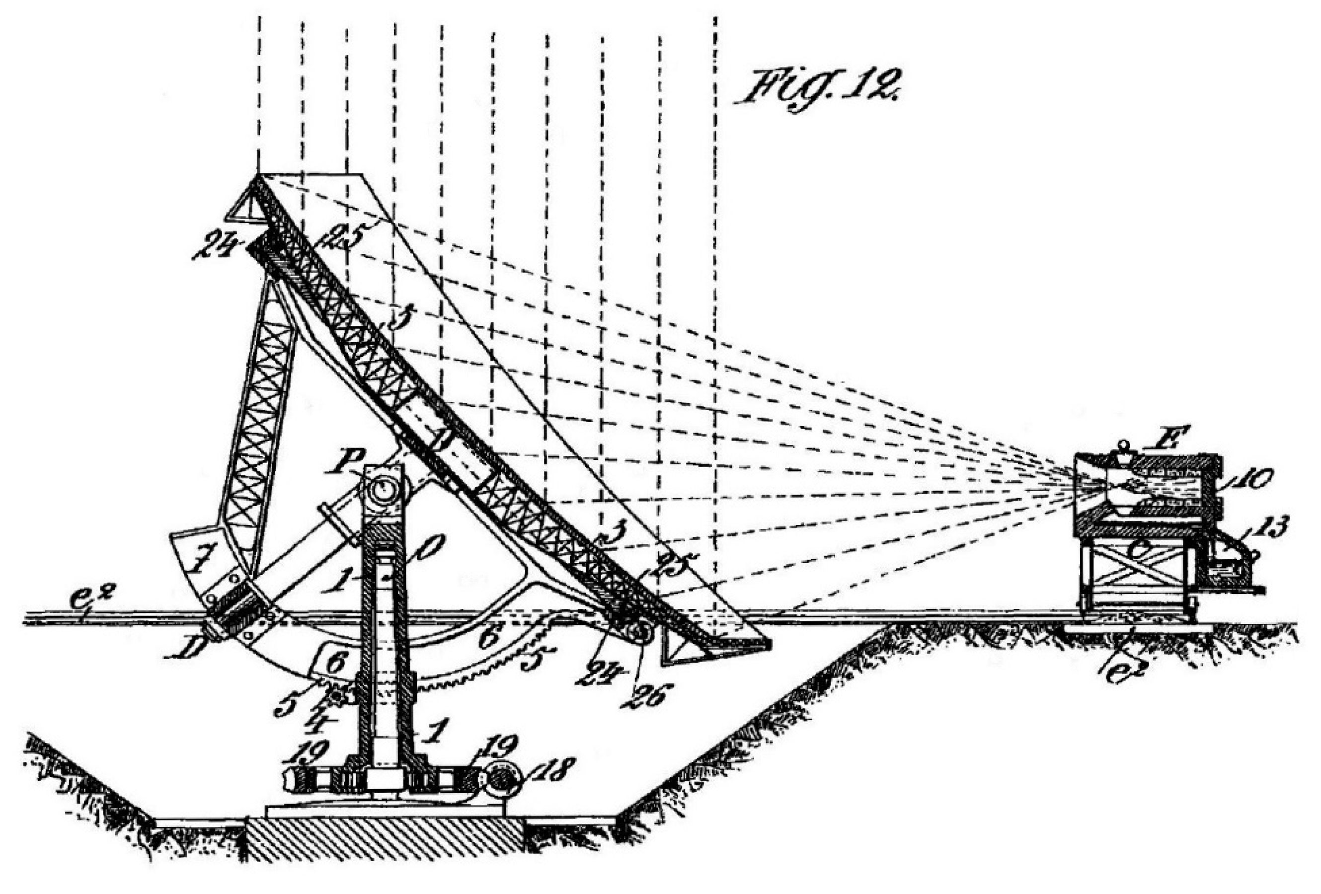
Geometrical optics, or ray optics, describes light propagation uniquely in terms of rays. Solar furnaces are examples of devices where the direct application of geometrical optics provides the basis for their design and optimization. The origin of modern solar furnaces dates back to the beginning of the 20th century, when the Portuguese priest Manuel Gomes (nicknamed ‘‘Father Himalaya” due to his tall figure) created and patented “an apparatus for making industrial use of the heat of the sun and obtaining high temperatures such as are required in metallurgical and chemical researches” [6,7]. In his UK [6] and US [7] patents, his invention is described as comprising a reflecting surface arranged to cause the solar rays to converge upon a confined focus placed in the centre of a furnace, crucible, or another receiver. An example of the figures in the UK patent is shown in Figure 1. For the 1904 Universal Expo of St. Louis, he built a huge device named Pyreliophorus, apparently similar to a large convex lens, where thousands of mirrors over a surface of 80 square meters concentrated solar energy up to a temperature of around 3500 °C, enough to melt many different types of materials, including metals and rocks. The Pyreliophorus installation was one of the main attractions on the Saint Louis world’s fair, where it was awarded with two gold medals and with one silver medal [8,9].

By the initiative of the French chemist Félix Trombe and his team, a so-called “solar furnace” was built in 1949 at the town of Mont-Louis, a commune in the French Pyrénées-Orientales. Some years later, on the model of the Mont-Louis furnace and using the results obtained there, a huge solar furnace was built (not very far from Mont-Louis) at Odeillo (Pyrénées-Orientales and Cerdagne near the Spanish border in the south of France). Work on the construction of the Odeillo solar furnace lasted from 1962 to 1968, and it was commissioned in 1970 [10]. This furnace could reach a power of one megawatt and nowadays continues serving as an installation for studying materials at very high temperatures. In a recent work by Levêque et al. [11], the characteristics of “solar furnaces”—in point-focusing solar concentration facilities located throughout the world, at universities, research institutes, and companies, and operating at concentrations relevant to solar thermochemistry—have been summarized. More recently (2018), state-of-the-art uses of concentrated solar energy applied to materials science and metallurgy have been comprehensively reviewed by Fernández-González et al. [12].

All high-flux solar furnaces distributed throughout the world have been designed and constructed individually, i.e., on a one-by-one basis because there are several possible optical configurations that must take into account the geographical location, and the maximum power to be attained. In fact, as referred by Riveros-Rosas et al. [13], there is little information in the literature regarding the detailed optical analysis of the existing furnaces and discussing the considerations and methods that led to their final optical design. In order to achieve the design targets, several possible configurations [14,15] can be analysed and the optical characteristics of the system can be optimized by means of ray tracing simulations, which is the scope of the present work.

2. Ray Tracing Simulation

Early academic research in nonimaging optical mathematics seeking closed form solutions was probably first published in textbook form by Welford and Winston [16]. Unlike traditional imaging optics, the techniques of nonimaging optics do not attempt to form an image of the source; instead, nonimaging optics is the branch of optics concerned with the optimal transfer of light radiation between a source and a target, aiming at developing techniques for maximizing the collecting power.

Ray-tracing computer programs, which simulate the propagation of light through three-dimensional models of optical systems, have their origin in the 1960s [17,18], but then, since 1970, with the advent of means for rapid computation, it became possible to simulate a wide range of optical phenomena (physical or geometrical) in contexts so diversified as electromagnetism, optics, astronomy, meteorology, environment, or architecture, as revealed in the literature, e.g., References [19,20,21,22,23,24,25]. Consequently, many commercial or free software packages have been developed to deal with this vast domain of topics, for example, CUtrace [26]; OpenRayTrace [27]; OTSun project [28]; Ray Optics Module: an add-on to the COMSOL Multiphysics software [29]; Ray Optics Simulation [30]; Solstice Program [31]; SolTrace [32]; Stellar Software [33]; Tonatiuh [34]; Zemax’ OpticStudio [35]. However, these general-purpose computer packages are more complex to use and less pedagogic than a simple computer program specifically designed from scratch to study a limited class of problems. In this work, we wrote software to exactly fulfil our own needs, which can easily be extended to analyse increasingly complex and diversified optical systems. Our motivation is to contributing to optimize high-flux solar furnaces using software that is simultaneously powerful, simple and elegant, and, at the same time, keeping a maximum degree of freedom and control in our modelling choices. We explained the relevant mathematical details so other users can build their own software to pursue their own goals. The final objective is to solve specific problems, such as the need for better temperature homogenisation in solar furnaces [36,37] or to improve the design of the focusing layout [38].

In this work, we discuss three models of geometrical optics that can be used to simulate the way a solar furnace collects and concentrates solar radiation. Based on their working principles, we designate these models as (1) spherical emission; (2) spherical reflection; (3) paraboloid reflection. These models can be used separately or combined in more complex simulations. Their implementation in software is simple once the mathematical principles supporting them are well understood. These principles are explained in detail in the next sections for the three models. For speed and simplicity, these models were implemented in the C programming language in a Linux operating system. All three ray-tracing algorithms reported here are O(N), in the range tested, from N = 10⁵ to N = 10⁹: the computer time required scales linearly with the number of rays N. Less than 1000 lines of C code were needed to implement all the models and experiments reported in this work. As an example, to simulate one hundred million rays (10⁸), in a simple Intel i3 powered notebook, it takes about 66 s (spherical emission), 59 s (spherical reflection) and 62 s (paraboloid reflection).

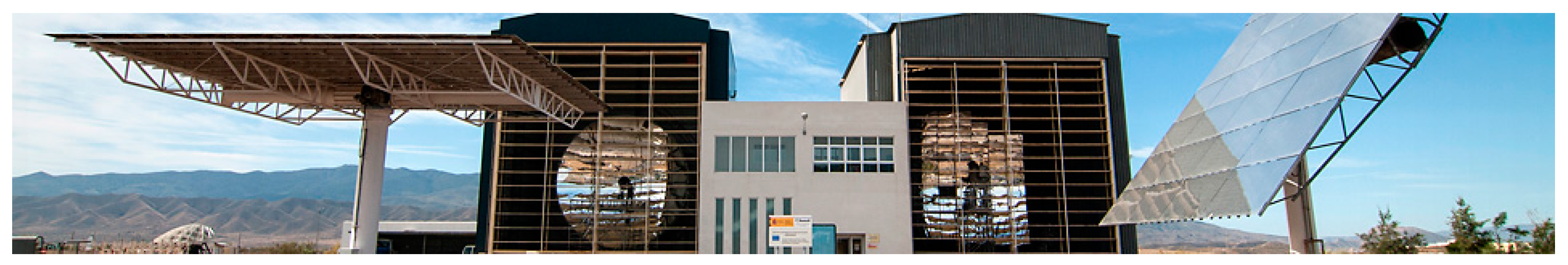
Examples of studies that can be undertaken with these models are demonstrated for the high-flux solar furnace SF60 (see Figure 2) at Plataforma Solar de Almería, in Spain. The main components of the solar furnace are flat heliostat; slat attenuator (also called “shutter”); parabolic concentrator and a test table.

3. Models and Simulations

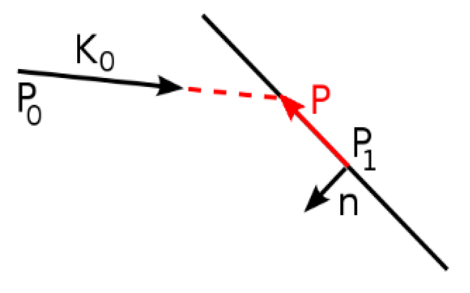
Any mathematical model of three-dimensional geometrical optics must solve two basic problems. The first is, given a wave vector K₀ travelling through some point P₀, where does it intersect a plane with a normal unit vector n that includes some point P₁ (see Figure 3)?

The point P where the wave vector intersects the plane can be obtained by first calculating the scaling factor s as described by the following equations:

$$\overrightarrow{{\mathrm{P}}_0}+s\overrightarrow{{\mathrm{K}}_0}=\overrightarrow{\mathrm{P}}$$

(1)

$$(\overrightarrow{\mathrm{P}}-\overrightarrow{{\mathrm{P}}_1})·\overrightarrow{\mathrm{n}}=0$$

(2)

x_o + sk_ox = x, y_o + sk_oy = y, z_o + sk_oz = z

(3)

n_x(x − x₁) + n_y(y − y₁) + n_z(z − z₁) = 0

(4)

n_x[(x₀ + skx_0x) − x₁] + n_y[(y₀ + sk_0y) − y₁] + n_z[(z₀ + sk_0z)−z₁] = 0

(5)

n_x(x₀ − x₁) + sn_xk_ox + n_y(y₀ − y₁) + sn_yk_oy + n_z(z₀ − z₁) + sn_zk_oz = 0

(6)

$$s=\frac{{\mathrm{n}}_{\mathrm{x}}({\mathrm{x}}_1-{\mathrm{x}}_0)+{\mathrm{n}}_{\mathrm{y}}({\mathrm{y}}_1-{\mathrm{y}}_0)+{\mathrm{n}}_{\mathrm{z}}({\mathrm{z}}_1-{\mathrm{z}}_0)}{{\mathrm{n}}_{\mathrm{x}}{\mathrm{k}}_{0\mathrm{x}}+{\mathrm{n}}_{\mathrm{y}}{\mathrm{k}}_{0\mathrm{y}}+{\mathrm{n}}_{\mathrm{z}}{\mathrm{k}}_{0\mathrm{z}}}$$

(7)

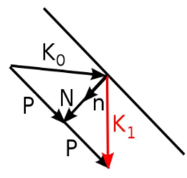
The second problem is, given some wave vector K₀ intersecting a plane perpendicular to a normal unit vector n, what is the output wave vector K₁ if specular reflection is assumed (see Figure 4)?

Assuming specular reflection, the output wave vector K₁ can be evaluated from the following vector equations:

$$\overrightarrow{{\mathrm{K}}_{\mathrm{o}}}+\overrightarrow{{\mathrm{K}}_1}=2\overrightarrow{\mathrm{P}}$$

(8)

$$(\overrightarrow{{\mathrm{K}}_{\mathrm{o}}}+\overrightarrow{\mathrm{N}})=\overrightarrow{\mathrm{P}}$$

(9)

$$\overrightarrow{\mathrm{N}}=(-\overrightarrow{{\mathrm{K}}_{\mathrm{o}}}·\overrightarrow{\mathrm{n}})\overrightarrow{\mathrm{n}}$$

(10)

$$\overrightarrow{{\mathrm{K}}_1}=-\overrightarrow{{\mathrm{K}}_{\mathrm{o}}}+2(\overrightarrow{{\mathrm{K}}_{\mathrm{o}}}+\overrightarrow{\mathrm{N}})=\overrightarrow{{\mathrm{K}}_{\mathrm{o}}}+2(-\overrightarrow{{\mathrm{K}}_{\mathrm{o}}}·\overrightarrow{\mathrm{n}})\overrightarrow{\mathrm{n}}$$

(11)

$$\overrightarrow{{\mathrm{K}}_1}=\overrightarrow{{\mathrm{K}}_{\mathrm{o}}}-2(\overrightarrow{{\mathrm{K}}_{\mathrm{o}}}·\overrightarrow{\mathrm{n}})\overrightarrow{\mathrm{n}}$$

(12)

Both answers to the above-mentioned problems/questions are required to simulate virtual detectors (measuring the radiation that reaches some point), to simulate specular reflexion (by plane or curved mirrors), or to determine the focal point after specular reflexion (namely by spherical or paraboloid surfaces).

An arbitrarily complex surface can always be tessellated, divided in many tiny triangles, each one with a normal vector perpendicular to the triangle’s surface. Identifying which triangle was intersected by a particular ray and calculating the reflexion using the triangle normal is a general method to simulate light reflexion by a surface. In this work, we wanted to simulate the light behaviour in a solar furnace using simple surfaces that can be handled analytically to reproduce the concentrator geometry. As cylindrical curvatures lack the required symmetry, and paraboloid emission is essentially equivalent to paraboloid reflexion (due to its single focal point) we are left with the three models analysed in this work: (1) spherical emission; (2) spherical reflection; (3) paraboloid reflection.

3.1. Spherical Emission Model

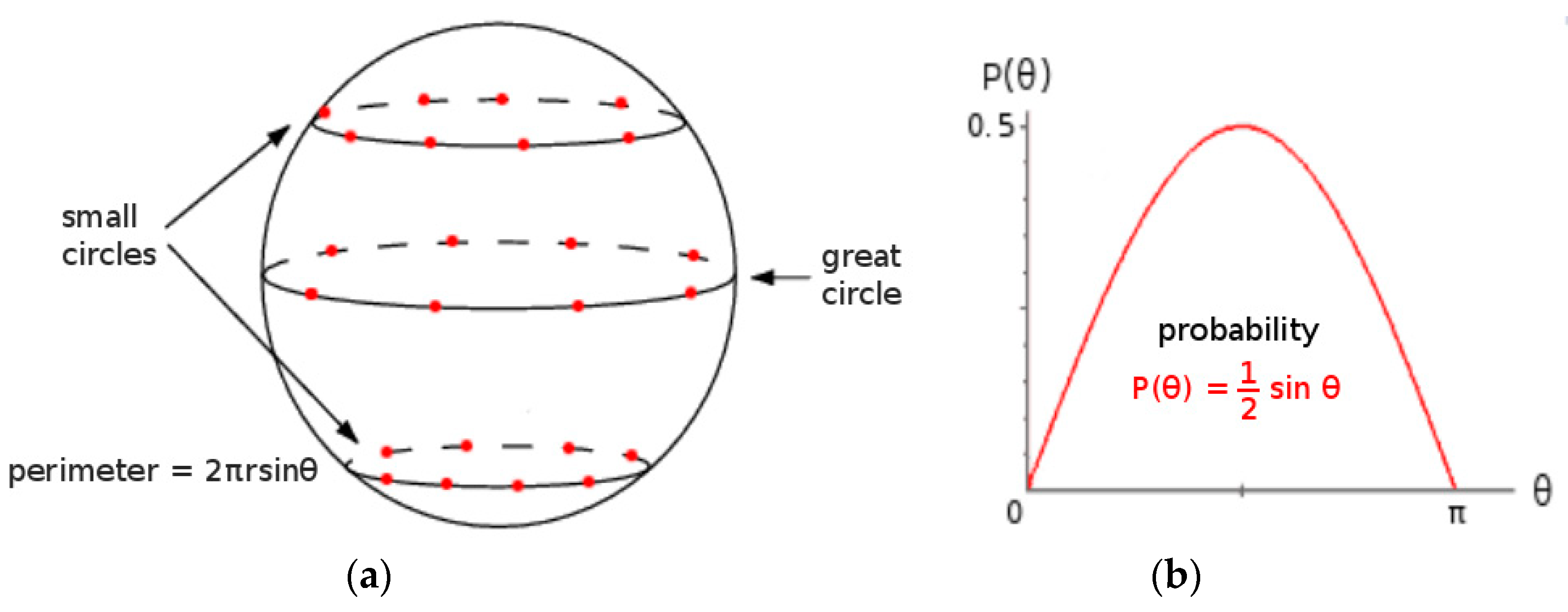
This model generates random points equally distributed over a spherical surface, interpreted as starting points for light rays pointing to the centre of the sphere, the focal point. To generate random points (r, χ_θ, χ_ϕ) over the surface using random numbers R_θ, R_ϕ between 0 e 1 (easily obtained in any programming language), it is correct to set χ_ϕ = 2π R_ϕ but not χ_θ = π R_θ because the point density would be higher over the poles than near the equator, as illustrated in Figure 5. The number of points generated must be proportional to the perimeter of the circumference describing each latitude θ: P(θ) = A2πrsinθ = Bsinθ, where A,B are constants. Normalising this probability distribution between 0 and π (B = 1/2), integrating between 0 and χ_θ and equalizing to R_θ, we obtain an expression χ_θ = arccos (1 − 2 R_θ) for the angle χ_θ as a function of the random number R_θ.

However, as the model emulates light coming from a curved mirror (the concentrator), the angle θ is restricted to some range [0, M] which is [0°, 38°] for the solar furnace SF60. By rewriting the calculations for an arbitrary angle M (between 0 and π), a final expression is obtained for χ_θ that, together with χ_ϕ, can be used to generate random points equally distributed over a spherical surface in the latitude range [0, M]:

$${{\displaystyle \int }}_0^{M}Bsin\mathsf{\theta }\mathrm{d}\mathsf{\theta }=-Bcos\mathsf{\theta }{|}_o^M=-B(cosM-1)=1\underset{}{\Rightarrow }B=\frac{1}{1-cosM}$$

(13)

$$R_{\mathsf{\theta }}={{\displaystyle \int }}_0^{{\mathsf{\chi }}_{\mathsf{\theta }}}\frac{1}{1-cosM}sin\mathsf{\theta }\mathrm{d}\mathsf{\theta }=\frac{1}{1-cosM}-cos\mathsf{\theta }{|}_o^{{\mathsf{\chi }}_{\mathsf{\theta }}}=\frac{cos{\mathsf{\chi }}_{\mathsf{\theta }}-1}{cosM-1}\underset{}{\iff }$$

$$\underset{}{\iff }cos{\mathsf{\chi }}_{\mathsf{\theta }}=1+R_{\mathsf{\theta }}(cosM-1)\underset{}{\iff }{\mathsf{\chi }}_{\mathsf{\theta }}=arccos(1+R_{\mathsf{\theta }}(cosM-1))$$

(14)

The probability distribution P(θ) = A2πrsinθ = Bsinθ must be normalized so B = 1/(1 − cosM). Random numbers χ_θ will follow the P(θ) distribution if χ_θ = arccos [1 + R_θ (cosM − 1)], where R_θ is a random number between 0 and 1.

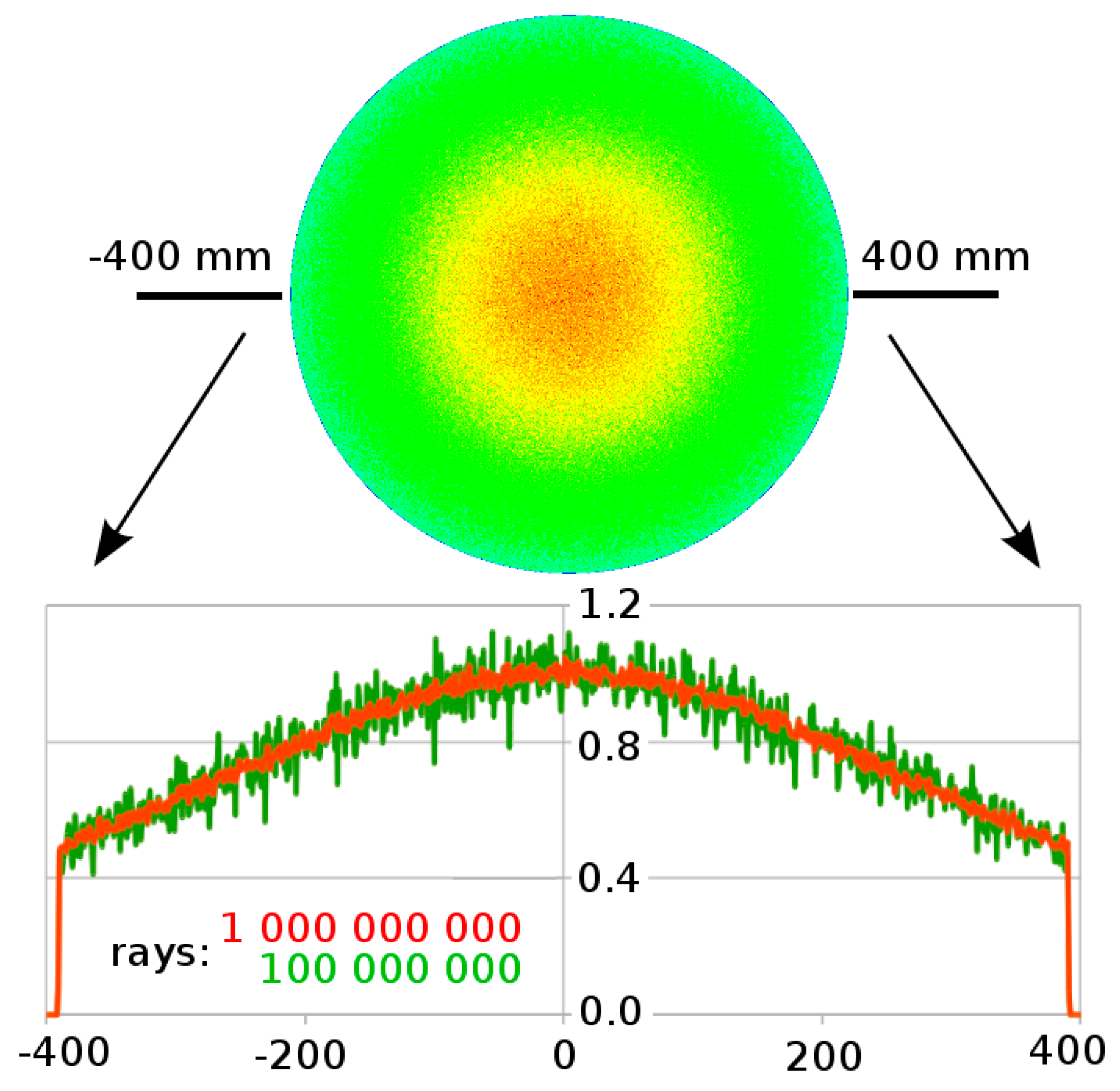
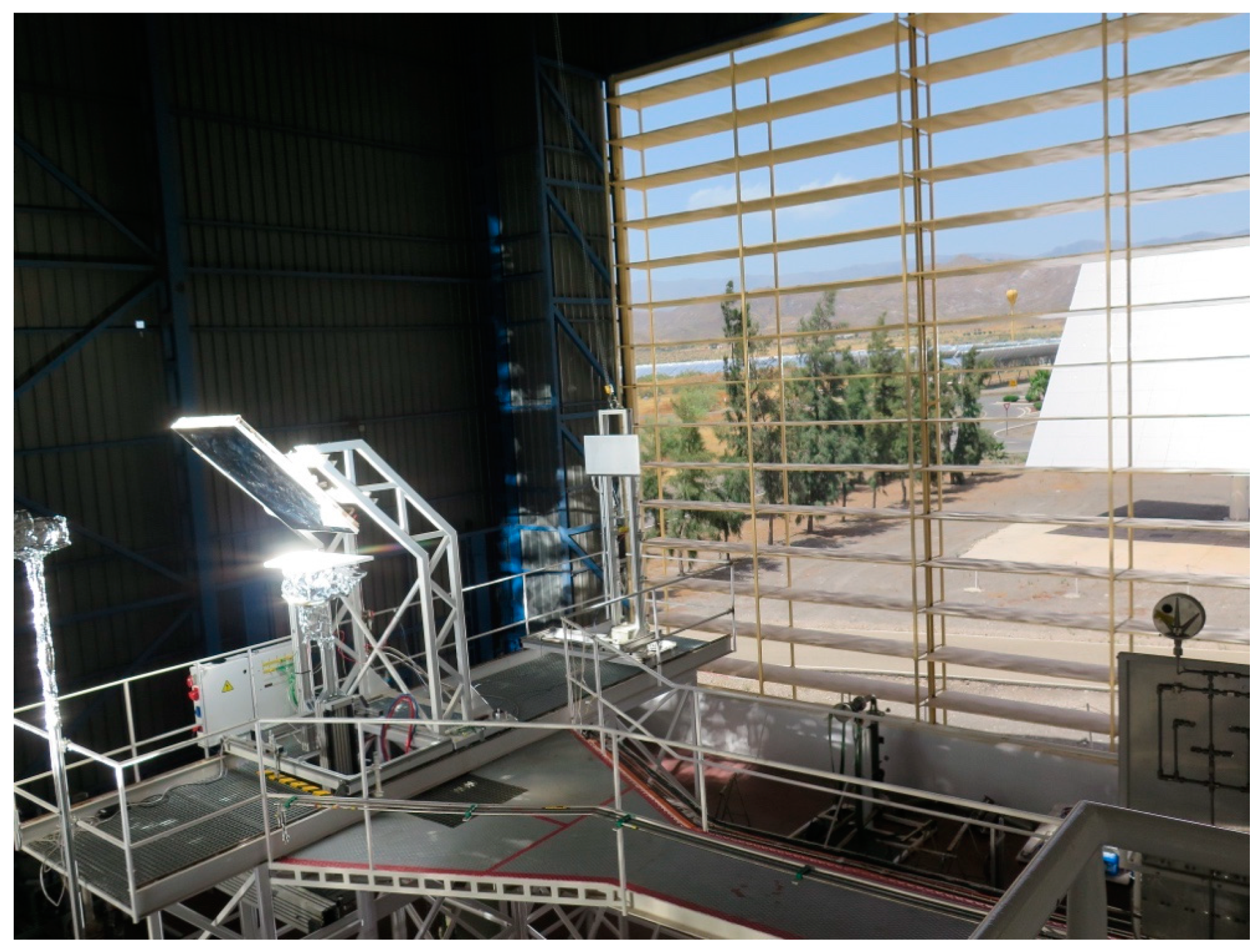
Using this model, we can calculate the radiation reaching the 45° mirror installed at the SF60 furnace, at 500 mm from the focal point (see Figure 6), that redistributes the concentrated radiation to a table of experiments below. The results obtained for a vertical detector are shown in Figure 7. A detector is simulated as a photographic camera, indicating its rectangular dimensions x,y and the three vectors: centre, target and top.

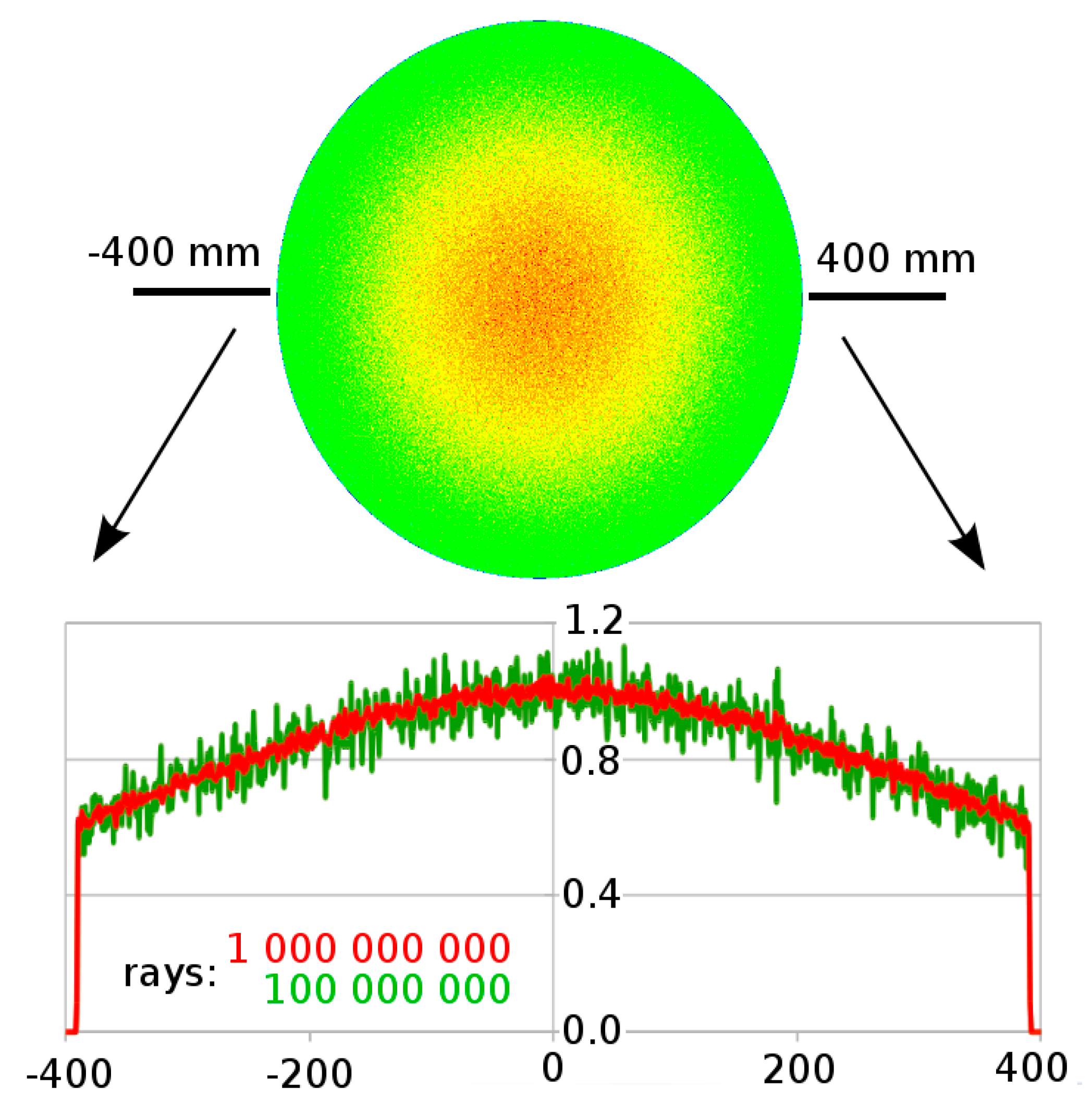
As expected, a circle is illuminated with a higher concentration in the middle. Increasing the number of rays by 10 times, from 10⁸ to 10⁹, produces the same radiation profile, just decreasing the statistical fluctuations, as depicted in Figure 7. To compare the two experiments, each curve (data set) was scaled between 0 and 1, dividing by the average value over the 10% central region (between −40 mm and +40 mm).

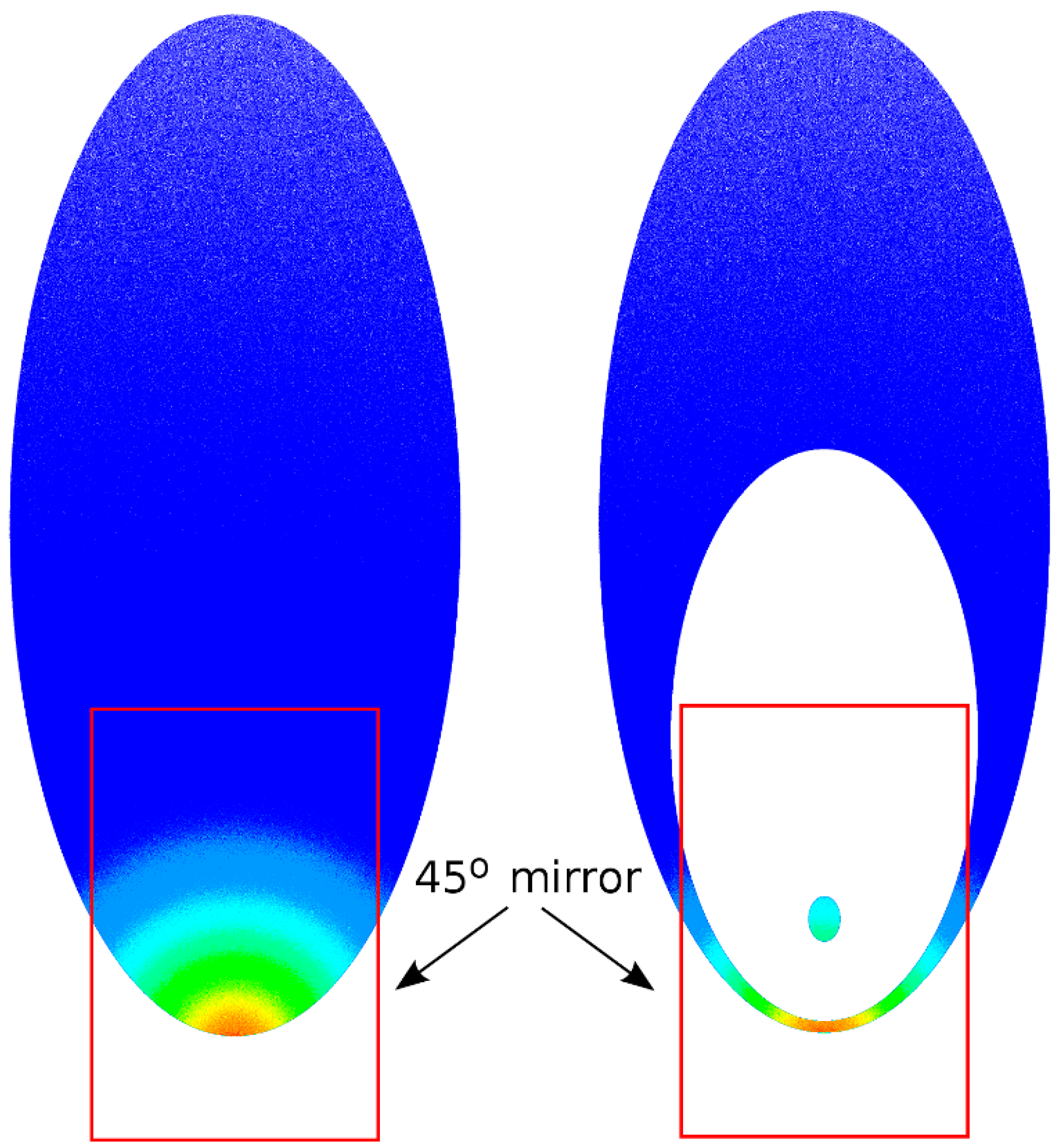
The results measured (forming an ellipse) for a detector aligned with the mirror are presented in Figure 8. These results show that the mirror loses 16.9% of the concentrated radiation when it is positioned in a symmetrical position, relative to the concentrator axis. This happens because the cone of acceptance of radiation coming from the concentrator collects radiation until a maximum angle of 38° (the rim angle), which is close to the 45° orientation of the mirror. As a result, the upper rays reach the mirror plane still far from the focal point and need a wide region to be collected, while the lower rays reach the mirror plane very close to the focus in a small region with high intensities, as shown in Figure 8. According to this model, raising the mirror 290 mm along the 45° plane maximizes the radiation collected by the mirror. Raising even more the mirror, the lower radiation, highly concentrated, is lost. In practice, the best option is probably to raise the mirror about 200 mm only, to make sure that all the lower radiation is collected.

3.2. Spherical Reflection Model

The key geometric aspects of the spherical reflection model are shown in Figure 9.

The input rays are reflected as prescribed by the following equations (extended to 3 dimensions):

$$(0,f)=(\mathrm{x},\mathrm{y})+s\overrightarrow{{\mathrm{K}}_1},\overrightarrow{{\mathrm{K}}_1}=\overrightarrow{{\mathrm{K}}_{\mathrm{o}}}-2(\overrightarrow{{\mathrm{K}}_{\mathrm{o}}}·\overrightarrow{\mathrm{n}})\overrightarrow{\mathrm{n}},\overrightarrow{{\mathrm{K}}_0}=(0,\mathrm{k}),\overrightarrow{\mathrm{n}}=(-\frac{\mathrm{x}}{\mathrm{r}},-\frac{\mathrm{y}}{\mathrm{r}})$$

(15)

$$(0,f)=(\mathrm{x},\mathrm{y})+s(0,\mathrm{k})-2s(0,\mathrm{k})·(-\frac{\mathrm{x}}{\mathrm{r}},-\frac{\mathrm{y}}{\mathrm{r}})·(-\frac{\mathrm{x}}{\mathrm{r}},-\frac{\mathrm{y}}{\mathrm{r}})=(\mathrm{x},\mathrm{y}+s\mathrm{k})+2s\frac{\mathrm{ky}}{\mathrm{r}}(-\frac{\mathrm{x}}{\mathrm{r}},-\frac{\mathrm{y}}{\mathrm{r}})$$

(16)

$$\{\begin{array}{c}0=\mathrm{x}-2s\mathrm{k}\frac{\mathrm{xy}}{{\mathrm{r}}^2}\underset{}{\Rightarrow }s=\frac{{\mathrm{r}}^2}{2\mathrm{ky}}\\ f=\mathrm{y}+s\mathrm{k}(1-2\frac{{\mathrm{y}}^2}{{\mathrm{r}}^2})=\mathrm{y}+\frac{{\mathrm{r}}^2}{2\mathrm{ky}}\mathrm{k}(1-2\frac{{\mathrm{y}}^2}{{\mathrm{r}}^2})=\mathrm{y}+\frac{{\mathrm{r}}^2}{2\mathrm{y}}-\mathrm{y}=\frac{\mathrm{r}/2}{\mathrm{y}/\mathrm{r}}\underset{}{\Rightarrow }f=\frac{\mathrm{r}/2}{cos\mathsf{\alpha }}\end{array}$$

(17)

The focal distance for the reflected rays is given by f = r/(2cosα) so f depends on the angle α. Therefore, the reflected rays focus on a line instead of a point. For example, f = r for α = 60° and f = rcos45° for α = 45°. Outer rays (with larger α) focus further away from the minimum focus (r/2) than inner rays; so the rays must cross, producing complex and surprising intensity patterns.

Random points can be generated in a circle of diameter D to simulate the parallel rays coming from the heliostat that illuminate the projected circle of the spherical concentrator. In the case of solar furnace SF60, the focal distance is F = 7450 mm (the length between the concentrator and the closer focus point) and the maximum angular aperture is M = 38°, so D = 10295 mm (see Figure 10):

$$\begin{array}{r}tan\mathsf{\beta }\frac{\mathrm{r}sin\mathsf{\alpha }}{\mathrm{r}cos\mathsf{\alpha }-\frac{\mathrm{r}}{2cos\mathsf{\alpha }}}=\frac{sin\mathsf{\alpha }}{\frac{2cos{}^2\mathsf{\alpha }-1}{2cos\mathsf{\alpha }}}=\frac{2sin\mathsf{\alpha }cos\mathsf{\alpha }}{cos{}^2\mathsf{\alpha }+cos{}^2\mathsf{\alpha }-cos{}^2-sin{}^2\mathsf{\alpha }}=\\ =\frac{sin2\mathsf{\alpha }}{cos2\mathsf{\alpha }}=tan2\mathsf{\alpha }\stackrel{}{\Rightarrow }\mathsf{\beta }=2\mathsf{\alpha }\end{array}$$

(18)

$$\mathsf{\beta }=38\text{° }\underset{}{\Rightarrow }\mathsf{\alpha }=19\text{°}$$

(19)

$$F=7450\mathrm{mm}=\mathrm{r}-\frac{\mathrm{r}}{2cos\mathsf{\alpha }}=\mathrm{r}(1-\frac{1}{2cos19°})=0.4712\mathrm{r}\underset{}{\Rightarrow }\mathrm{r}=15811\mathrm{mm}$$

(20)

D = 2 r sin α = 2 × 15811 × sin 19° = 10295 mm

(21)

The length of the focal line is r/2(1/cosα − 1) = r/2 − F. For SF60 the length of the focal line becomes 456 mm. The light intensity increases slightly from r/2cos19° (the focal point closer to the concentrator) to r/2 (the focal point closer to the centre of the sphere), as shown in Figure 11 for a longitudinal plane detector.

The radiation reaching a vertical (transversal) detector located at the position of the 45° mirror (see Figure 6) is shown in Figure 12. As before (Figure 7), each curve was scaled between 0 and 1, dividing by the average value over the 10% central region (between –40 mm and +40 mm). The profile of intensity obtained for this model is surprising because the intensity increases from the centre to the periphery, rising fast near the boundary at 38°. This profile strongly depends on the focal distance. This occurs because the outer rays focus before the inner rays so they must cross, increasing the intensity in the outer regions.

The spherical reflection model is interesting and certainly important to simulate reflecting spherical surfaces. However, it cannot be used to simulate the geometries and optical behaviour usually found in solar furnaces.

3.3. Paraboloid Reflection Model

The key geometric aspects of the paraboloid reflection model are shown in Figure 13.

The input rays are reflected as prescribed by the following equations (extended to 3 dimensions):

$$(0,f)=(\mathrm{x},\mathrm{y})+s\overrightarrow{{\mathrm{K}}_1},\overrightarrow{{\mathrm{K}}_1}=\overrightarrow{{\mathrm{K}}_{\mathrm{o}}}-2(\overrightarrow{{\mathrm{K}}_{\mathrm{o}}}·\overrightarrow{\mathrm{n}})\overrightarrow{\mathrm{n}},\overrightarrow{{\mathrm{K}}_0}=(0,-\mathrm{k}),\mathrm{y}={\mathrm{ax}}^2$$

(22)

$$\overrightarrow{\mathrm{n}}=(\frac{-2\mathrm{ax}}{\sqrt{4{\mathrm{a}}^2{\mathrm{x}}^2+1}},\frac{1}{\sqrt{4{\mathrm{a}}^2{\mathrm{x}}^2+1}})$$

(23)

$$F=\mathrm{y}-{\mathrm{ax}}^2=0\underset{}{\Rightarrow }\overrightarrow{N}=[\mathrm{dF}/\mathrm{dx}\mathrm{dF}/\mathrm{dy}]=[-2\mathrm{ax}1]$$

(24)

$$(0,f)=(\mathrm{x},\mathrm{y})+s(0,-\mathrm{k})-2s(0,-\mathrm{k})·(\frac{-2\mathrm{ax}}{\sqrt{4{\mathrm{a}}^2{\mathrm{x}}^2+1}},\frac{1}{\sqrt{4{\mathrm{a}}^2{\mathrm{x}}^2+1}})(\frac{-2\mathrm{ax}}{\sqrt{4{\mathrm{a}}^2{\mathrm{x}}^2+1}},\frac{1}{\sqrt{4{\mathrm{a}}^2{\mathrm{x}}^2+1}})$$

(25)

$$(0,f)=(\mathrm{x},\mathrm{ax}{}^2)+(0,-\mathrm{k}s)+\frac{2\mathrm{k}s}{\sqrt{4{\mathrm{a}}^2{\mathrm{x}}^2+1}}(\frac{-2\mathrm{ax}}{\sqrt{4{\mathrm{a}}^2{\mathrm{x}}^2+1}},\frac{1}{\sqrt{4{\mathrm{a}}^2{\mathrm{x}}^2+1}})$$

(26)

$$(0,f)=(\mathrm{x},\mathrm{ax}{}^2)+(0,-\mathrm{k}s)+(\frac{-4\mathrm{akx}s}{4{\mathrm{a}}^2{\mathrm{x}}^2+1},\frac{2\mathrm{k}s}{4{\mathrm{a}}^2{\mathrm{x}}^2+1})$$

(27)

$$\{\begin{array}{c}0=\mathrm{x}+0-\frac{4\mathrm{akx}s}{4{\mathrm{a}}^2{\mathrm{x}}^2+1}\underset{}{\Rightarrow }s=\frac{4{\mathrm{a}}^2{\mathrm{x}}^2+1}{4\mathrm{ak}}\\ f=\mathrm{a}\mathrm{x}{}^2-\mathrm{k}\frac{4{\mathrm{a}}^2{\mathrm{x}}^2+1}{4\mathrm{ak}}+\frac{2\mathrm{k}}{4{\mathrm{a}}^2{\mathrm{x}}^2+1}\frac{4{\mathrm{a}}^2{\mathrm{x}}^2+1}{4\mathrm{ak}}=-\frac{1}{4\mathrm{a}}+\frac{1}{2\mathrm{a}}\underset{}{\Rightarrow }f=\frac{1}{4\mathrm{a}}\end{array}$$

(28)

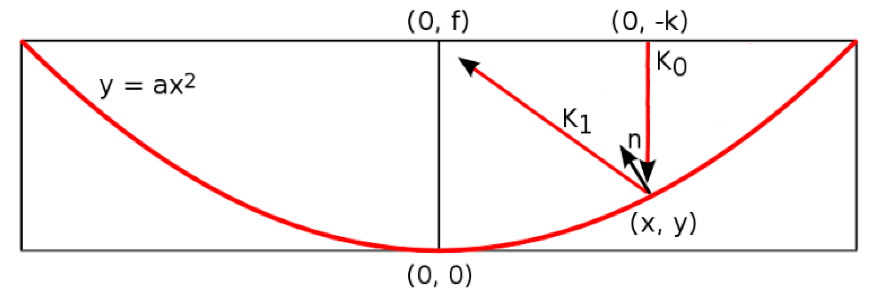
When vertical rays (0, −k) are reflected by a parabola y = ax², the focal point is constant, f = 1/(4a), one of the most remarkable properties of a parabola (2D) or paraboloid (3D). As reflected rays are all converging in the same point, this model is expected to have a behaviour similar to the model of spherical emission, where the focal point, by construction, is also unique.

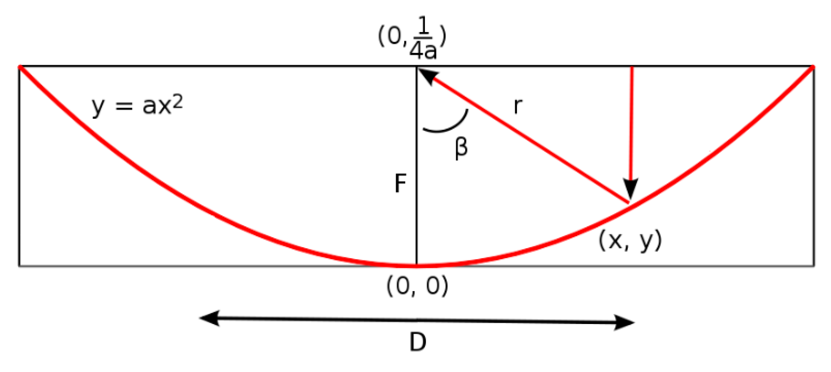
As in the spherical reflection model, random points can be generated in a circle of diameter D to simulate the parallel rays coming from the heliostat that illuminate the projected circle of the paraboloid concentrator (see Figure 14). In the case of the solar furnace SF60, the focal distance is F = 7450 mm and the maximum angular aperture is M = 38°, so a = 1/29800 mm and D = 10260 mm:

$$\{\begin{array}{c}0+\mathrm{r}sin\mathsf{\beta }=x\\ \frac{1}{4\mathrm{a}}-\mathrm{r}cos\mathsf{\beta }=y\end{array}\{\begin{array}{c}\mathrm{r}=\frac{x}{sin\mathsf{\beta }}\\ \frac{1}{4\mathrm{a}}-\frac{x}{sin\mathsf{\beta }}cos\mathsf{\beta }=\mathrm{ax}{}^2\end{array}$$

(29)

$$\mathrm{ax}{}^2+\frac{x}{tan\mathsf{\beta }}-\frac{1}{4\mathrm{a}}=0\underset{}{\Rightarrow }x=\frac{\frac{-1}{tan\mathsf{\beta }}\pm \sqrt{(\frac{1}{tan\mathsf{\beta }}){}^2-4\mathrm{a}\frac{-1}{4\mathrm{a}}}}{2\mathrm{a}}=\frac{\frac{-1}{tan\mathsf{\beta }}\pm \sqrt{(\frac{1}{tan\mathsf{\beta }}){}^2+1}}{2\mathrm{a}}$$

(30)

$$F=7450\mathrm{mm}=\frac{1}{4\mathrm{a}}\underset{}{\Rightarrow }\mathrm{a}=\frac{1}{29800}\underset{}{\Rightarrow }\mathrm{y}=\frac{{\mathrm{x}}^2}{29800}$$

(31)

$$\mathsf{\beta }=38°\underset{}{\Rightarrow }\mathrm{x}=\frac{\frac{-1}{tan{38}^{°}}+\sqrt{(\frac{1}{tan{38}^{°}})2+1}}{2/29800}=5130\mathrm{mm}\underset{}{\Rightarrow }D=2\mathrm{x}=10260\mathrm{mm}$$

(32)

We note that the diameter D determined analytically by this model and by the previous one are almost equal, differing only by 35 mm. This is interesting, considering that the two models are quite different, particularly the aspects related to the focal distance.

As for the previous models, we measured (Figure 15) the radiation reaching the 45° mirror with a vertical detector, using two different numbers of sampling rays. As before (Figure 7 and Figure 12), each curve was scaled between 0 and 1, dividing by the average value over the 10% central region (between –40 mm and +40 mm). As expected, the profile remains the same after increasing the number of reflected rays by 10 times, as observed before for the spherical emission model. The results obtained are indeed very similar to those obtained for the spherical emission model (Figure 7). This paraboloid profile is just slightly more flat than the spherical profile (the energy loss using the mirror of Figure 8 raises to 18.0%). This is interesting considering that the two models are very different from the mathematical point of view.

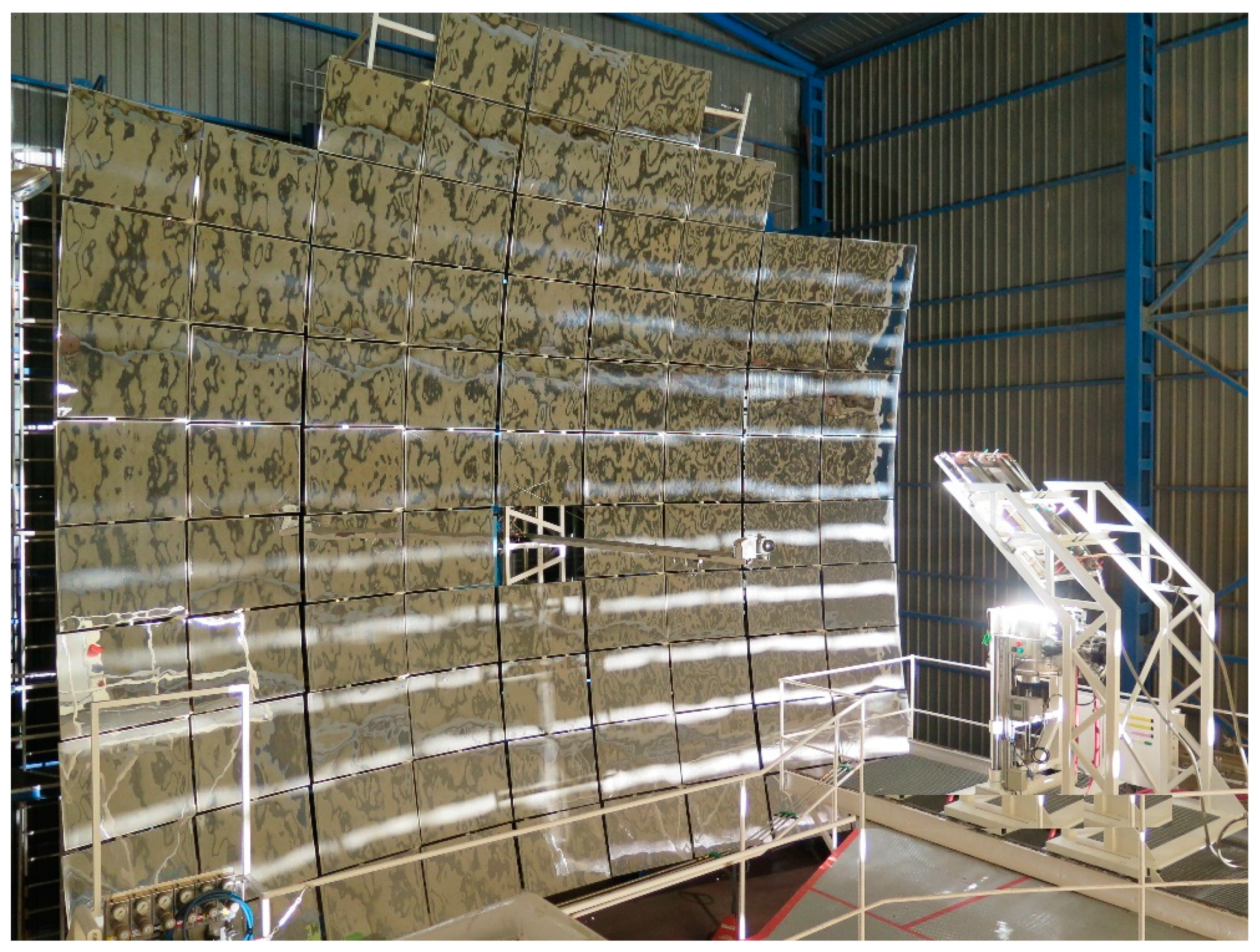
Unlike the spherical emission model that can be used only to simulate light events occurring after the concentrator, the paraboloid reflection model can be used to study events occurring after the heliostat. As an example, we analysed the light profile formed at the 45° flat mirror (500 mm from the focal point) when the 15 attenuation shutters that control the entrance of light to the solar furnace (see Figure 16) are only 90% open. The results are reported in Figure 17. The vertical circle (on the left) shows uniform gaps with 7 mm, while the 45° ellipse (on the right) shows decreasing gaps, with 75 mm at the top and 4 mm at the bottom. At the SF60 furnace, the sample is usually positioned 25 mm above the focal distance, so these effects are expected to be small but not negligible.

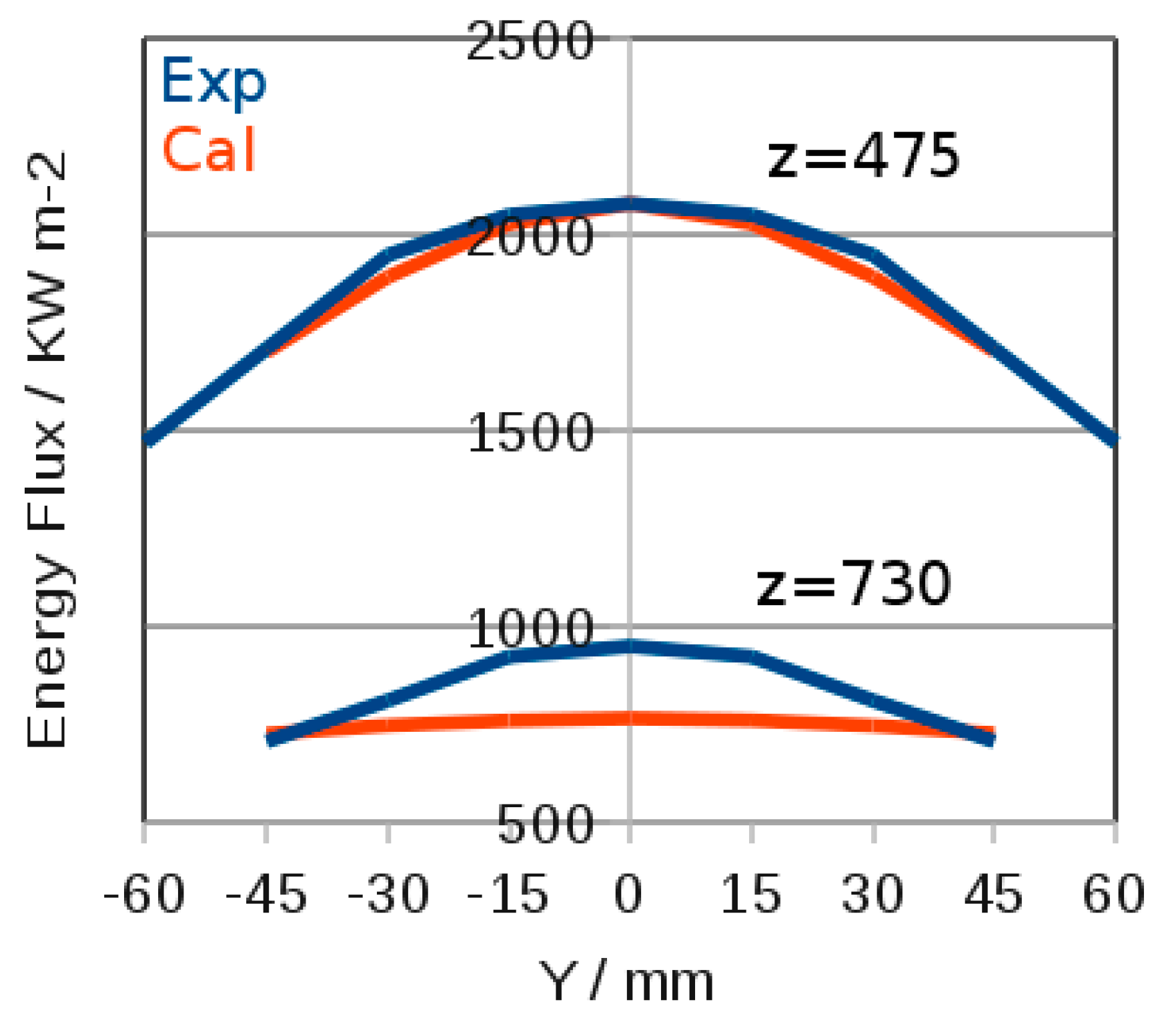
As another example, Figure 18 compares the experimental data obtained with a radiometer (Vatell Thermogage 1000-4, with a sensitivity = 2 mV per W/cm²), with a circular measurement area (diameter = 5/8 in = 15.9 mm), with data calculated using our software. The results obtained for the flux of energy (in kW/m²), 475 mm and 730 mm below the 45° mirror, for the SF60 solar furnace, are quite satisfactory given the natural limitations of the experimental infrastructure.

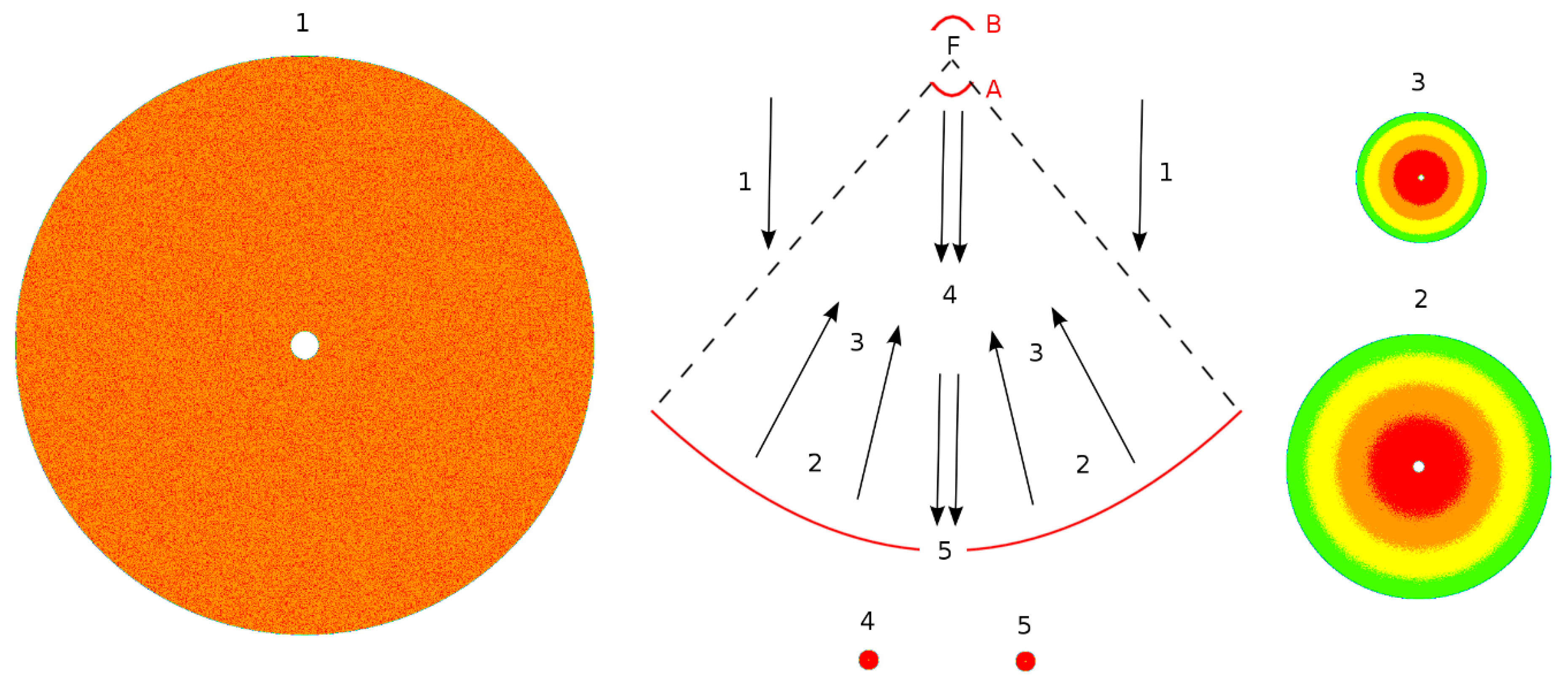
Finally, we show how this software can contribute to developing new devices such as the flux concentrator shown in Figure 19, with a geometry similar to SF60 (a focal distance of 7450 mm and a rim angle of 38°). The parallel rays (1) coming from the sun are reflected in the large, concave, paraboloid, before being concentrated (2 and 3) to the focal point F. If these rays are reflected by a small paraboloid with the same focal point of the big one—a convex such as paraboloid A or concave such as paraboloid B—then our calculations show that the reflected rays (4 and 5) are simultaneously highly concentrated and equally distributed over the narrow illuminated region (with a very small hole in the middle due to the shadow produced by the second paraboloid, probably too small to be detectable). For this example, we arbitrarily chose 250 mm for the projected radius of the small paraboloid, which seems adequate for the dimensions of SF60. If proven experimentally valid, this design circumvents one of the major issues with high flux concentrators: the Gaussian distribution was usually predicted for the radial flux of energy, making it difficult to obtain a homogeneous source of concentrated energy with these solar furnaces.

4. Conclusions and Prospects for Future Work

The 10⁹ rays used in our simulations proved enough to give an accurate description of the light behaviour which can be adequately compared to the experimental flux of energy in kW/m².

From our theoretical analyses, we may conclude that the spherical reflection model is very interesting due to its rich, complex behaviour that leads to surprising results, as the U shaped distribution of intensity. However, it is not appropriate to simulate high concentration solar furnaces such as SF60 with a distribution of flux of radiation that is maximum in the centre, with a single focal point. The spherical emission and paraboloid reflection models have the desired behaviour, showing similar results in spite of their totally different mathematical conceptions. The advantage of the paraboloid reflection over the spherical emission is that in the first model, the simulation starts at the heliostat while in the second model it starts only at the concentrator. Thus, optical phenomena occurring before the concentrator (for example, the effect of the partial overture of the attenuation shutters in the distribution of radiation reaching the sample) cannot be studied by the model of spherical emission. Moreover, it is well known that the curved mirror surfaces used to concentrate light in solar furnaces are usually built with a paraboloid geometry.

In future work, we intend to analyse the behaviour of multi-mirror devices by comparing simulation and experimental data. The goal is to contribute for the development of devices designed to homogenise the flux of radiation near the sample as much as possible (to equilibrate the temperatures), a critical issue in high concentration solar furnaces such as SF60. Our ray-tracing simulations allowed for the confirmation of the possibility to attain homogenous distribution of flux by means of double reflexion using two paraboloid surfaces.

References

- Rashed, R. A Pioneer in Anaclastics: Ibn Sahl on burning mirrors and lenses. Isis 1990, 81, 464–491. [Google Scholar] [CrossRef]
- Dijksterhuis, F.J. Christiaan Huygens and the Mathematical Science of Optics in the Seventeenth Century; Springer: Berlin/Heidelberg, Germany, 2004; ISBN 978-1-4020-2697-3. [Google Scholar]
- Young, T. The Bakerian Lecture. Experiments and calculations relative to physical optics. Philos. Trans. R. Soc. Lond. 1804, 94, 1–16. [Google Scholar] [CrossRef]
- Born, M.; Wolf, E. Principles of Optics: Electromagnetic Theory of Propagation, Interference and Diffraction of Light, 7th ed.; Cambridge University Press: Cambridge, UK, 1999. [Google Scholar]
- Hecht, E. Optics, 5th ed.; Pearson: London, UK, 2016. [Google Scholar]
- Himalaya, M.A.G. Improved Apparatus for Making Industrial Use of the Heat of the Sun and Obtaining High Temperatures. Patent GB190116181, 26 October 1901. Available online: https://worldwide.espacenet.com/publicationDetails/biblio?FT=D&date=19011026&DB=EPODOC&locale=en_EP&CC=GB&NR=190116181A&KC=A&ND=2# (accessed on 20 June 2019).
- Himalaya, M.A.G. Solar Apparatus for Producing High Temperatures. U.S. Patent 797,891, 22 August 1905. Available online: https://patents.google.com/patent/US797891 (accessed on 20 June 2019).
- Rodrigues, J. A conspiração solar do Padre Himalaya—Esboço biográfico dum português pioneiro da Ecologia (The Solar Conspiration of Father Himalaya—Biographic Outline of a Portuguese Pioneer in Ecology); Árvore—Cooperativa de Actividades Artísticas: Porto, Portugal, 1999; ISBN 972-9089-44-2. [Google Scholar]
- Tinoco, A. Portugal na Exposição Universal de 1904: O Padre Himalaia e o Pirelióforo. Cadernos de Sociomuseologia 2012, 42, 113–127, Edições Universitárias Lusófonas. Available online: http://hdl.handle.net/10437/4545 (accessed on 20 June 2019).
- Trombe, F.; Le Phat Vinh, A. Thousand kW solar furnace, built by the National Center of Scientific Research, in Odeillo (France). Sol. Energy 1973, 15, 57–61. [Google Scholar] [CrossRef]
- Levêque, G.; Bader, R.; Lipinski, W.; Haussener, S. High-flux optical systems for solar thermochemistry. Sol. Energy 2017, 156, 133–148. [Google Scholar] [CrossRef] [Green Version]
- Fernández-González, D.; Ruiz-Bustinza, I.; González-Gasca, C.; Piñuela-Noval, J.; Mochón-Csataños, J.; Sancho-Gorostiaga, J.; Verdeja, L.F. Concentrated solar energy applications in materials science and metallurgy. Sol. Energy 2018, 170, 520–540. [Google Scholar] [CrossRef]
- Riveros-Rosas, D.; Herrera-Vázquez, J.; Pérez-Rábago, C.A.; Arancibia-Bulnes, C.A.; Vázquez-Montiel, S.; Sánchez-González, M.; Granados-Agustín, F.; Jaramillo, O.A.; Estrada, C.A. Optical design of a high radiative flux solar furnace for Mexico. Sol. Energy 2010, 84, 792–800. [Google Scholar] [CrossRef]
- Llorente, J.; Ballestrín, J.; Vásques, A.J. A new solar concentrating system: Description, characterization and applications. Sol. Energy 2011, 85, 1000–1006. [Google Scholar] [CrossRef]
- Luque, S.; González-Aguilar, J.; Romero, M. Design of a calorimetric facility to assess volumetric receivers employing a 42 kW high flux solar simulator. In Proceedings of the ISES Solar World Conference 2017 and the IEA SHC Solar Heating and Cooling Conference for Buildings and Industry, Abu Dhabi, UAE, 29 October–2 November 2017; International Solar Energy Society: Breisgau, Germany, 2017. [Google Scholar] [CrossRef]
- Welford, W.T.; Winston, R. The Optics of Nonimaging Concentrators: Light and Solar Energy, 1st ed.; Academic Press: Cambridge, MA, USA, 1978. [Google Scholar]
- Spencer, G.H.; Murty, M.V.R. General ray-tracing procedure. J. Opt. Soc. Am. 1962, 52, 672–678. [Google Scholar] [CrossRef]
- Freniere, E.R.; Tourtellott, J. A brief history of generalized ray tracing. Proc. SPIE 1997, 3130, 170–178. [Google Scholar] [CrossRef]
- Howell, B.J.; Wilson, M.E. Automatic ray-surface intersection method. Appl. Opt. 1982, 21, 2184–2188. [Google Scholar] [CrossRef]
- Kerisit, S.; Rosso, K.M.; Cannon, B.D.; Gao, F.; Xie, Y.L. Computer simulation of the light yield nonlinearity of inorganic scintillators. J. Appl. Phys. 2009, 105, 114915. [Google Scholar] [CrossRef]
- Dlugach, J.; Mishchenko, M.I.; Liu, L.; Mackowski, D.W. Numerically exact computer simulations of light scattering by densely packed, random particulate media. J. Quant. Spectrosc. Radiat. Transf. 2011, 112, 2068–2078. [Google Scholar] [CrossRef] [Green Version]
- Jafrancesco, D.; Sansoni, P.; Francini, F.; Contento, G.; Privato, C.; Graditi, G.; Ferruzzi, D.; Mercatelli, L.; Sani, E.; Fontani, D. Mirrors array for a solar furnace: Optical analysis and simulation results. Renew. Energy 2014, 63, 263–271. [Google Scholar] [CrossRef]
- Bader, R.; Haussener, S.; Lipinski, W. Optical design of multisource high-flux solar simulators. J. Sol. Energy Eng. 2015, 137, 021012. [Google Scholar] [CrossRef]
- Danko, O.; Danko, V.; Kovalenko, A. Light focusing through a multiple scattering medium: Ab initio computer simulation. Proc. SPIE 2017, 10612, 1061216. [Google Scholar] [CrossRef]
- Jin, J.; Liu, M.K.; Lin, P.Z.; Fu, T.R.; Hao, Y.; Jin, H.G. Ultrahigh temperature processing by concentrated solar energy with accurate temperature measurement. Appl. Therm. Eng. 2019, 150, 1337–1344. [Google Scholar] [CrossRef]
- CUtrace. Available online: https://www.mathworks.com/matlabcentral/fileexchange/52820-cutrace (accessed on 8 May 2019).
- OpenRayTrace. Available online: http://openraytrace.sourceforge.net/ (accessed on 8 May 2019).
- Pujol-Nadal, R.; Martínez-Moll, V.; Moià-Pol, A.; Cardona, G.; Hertel, J.D.; Bonnín, F. OTSun Project: Development of a Computational Tool for High-resolution Optical Analysis of Solar Collectors. In Proceedings of the 11th ISES EUROSUN 2016 Conference, Palma, Spain, 11–14 October 2016; Martinez, V., Gonzalez, J., Eds.; International Solar Energy Society: Freiburg, Germany, 2017; pp. 989–999. [Google Scholar] [CrossRef]
- Ray Optics Module. Available online: https://www.comsol.com/ray-optics-module#cmm-optical-ray-tracing-software (accessed on 8 May 2019).
- Ray Optics Simulation, Developed by Rick Tu. Available online: https://ricktu288.github.io/ray-optics/simulator/ (accessed on 8 May 2019).
- Solstice—The Solar Plant Simulation Tool. Available online: https://www.meso-star.com/projects/solstice/solstice.html (accessed on 8 May 2019).
- SolTrace. Available online: https://www.nrel.gov/csp/soltrace.html (accessed on 8 May 2019).
- Stellar Software. Available online: https://www.stellarsoftware.com/ (accessed on 8 May 2019).
- Tonatiuh. Available online: http://iat-cener.github.io/tonatiuh/ (accessed on 8 May 2019).
- Zemax’ OpticStudio. Available online: https://customers.zemax.com/os/resources/learn/tutorials (accessed on 8 May 2019).
- Li, B.; Oliveira, F.A.C.; Rodríguez, J.; Fernandes, J.C.; Rosa, L.G. Numerical and experimental study on improving temperature uniformity of solar furnaces for materials processing. Sol. Energy 2015, 115, 95–108. [Google Scholar] [CrossRef]
- Oliveira, F.A.C.; Fernandes, J.C.; Rodríguez, J.; Cañadas, I.; Galindo, J.; Rosa, L.G. Temperature uniformity improvement in a solar furnace by indirect heating. Sol. Energy 2016, 140, 141–150. [Google Scholar] [CrossRef]
- Martins, C.A.B. Aparelho Concentrador e Estabilizador de Raios Solares e Sistema de Transmissão de um Feixe de Raios Solares Concentrados e Estabilizados que o Contém. Portuguese Patent Pending Request No. PT20160109071, 4 January 2016. Available online: https://pt.espacenet.com/searchResults?CY=pt&DB=EPODOC&F=0&FIRST=1&LG=pt&PN=PT109071&Submit=PESQUISAR&bookmarkedResults=true&locale=pt_pt&sf=n (accessed on 20 June 2019).
Figure 1.
One of the figures of Manuel Gomes’ British patent application [6].
Figure 2.
High-flux solar furnaces SF40 (left) and SF60 (right), at Plataforma Solar de Almería (Spain).
Figure 3.
A wave vector K0 going through a point P0 and intersecting a plane containing a point P1 and perpendicular to a normal unit vector n, intersects the plane in some point P.
Figure 4.
A wave vector K0 intersecting a plane perpendicular to a normal unit vector n, is reflected as some output wave vector K1, assuming specular reflection.
Figure 5.
The number of random points (a) generated in each circle should be proportional to its perimeter, so the probability (b) of occurrence should be maximum in the equator (θ = 90°) and minimum in the poles (θ = 0° and 180°).
Figure 6.
An indoor photo of the SF60 solar furnace, showing concentrator (left) and the 45° flat mirror (500 mm from the focal point) reflecting the concentrated solar radiation to the sample region below.
Figure 7.
Radiation reaching a vertical plane at the same position of the 45° mirror shown in Figure 6, after emitting 108 rays. Increasing the number of rays by 10 times improves the statistical quality without changing the intensity profile.
Figure 8.
Radiation reaching a 45° plane (the detector) aligned with the 45° mirror shown in Figure 6, after simulation with 108 rays. The left picture shows the whole illuminated ellipse (1250 mm × 2836 mm) while the right picture shows only the regions illuminated for central (0–5°) and outer (33–38°) angles.
Figure 9.
(a) The specular reflection of a vertical wave vector K0 by a spherical surface with a radius r originates a wave vector K1 that intersects the focal axis at x = 0 in a point f that depends on the angle α: f = r/(2cosα); (b) Specular reflection for 45° and 60°.
Figure 10.
The diameter D of the projected concentrator is calculated noting that the maximum aperture angle β is twice the angle α measured from the spherical centre and equalizing the experimental focal distance F to the minimum focal distance: r – r/(2cosα).
Figure 11.
After spherical reflection, the focal line starts at r/2cosα and ends at r/2 (the closest point to the spherical centre), with an intensity that increases slightly from start to end. For SF60 α = β/2 = 19° and the focal line totals 456 mm.
Figure 12.
Radiation reaching a vertical plane at the same position of the 45° mirror shown in Figure 6, after spherical reflection of 108 rays.
Figure 13.
The specular reflection of a vertical wave vector K0 by a paraboloid y = ax2 originates in a wave vector K1 that intersects the paraboloid axis always in the same focal point: f = 1/(4a).
Figure 14.
The diameter D of the projected concentrator can be calculated by solving the 2nd-degree polynomial equation resulting from the system to find the point (x, y) where the ray intersects the paraboloid.
Figure 15.
Radiation reaching a vertical plane at the same position of the 45° mirror shown in Figure 6, after reflecting 108 rays. Increasing the number of rays by 10 times improves the statistical quality without changing the intensity profile.
Figure 16.
Inside the SF60 solar furnace, showing the 45° flat mirror (left), the 15 shutter panels that control the level of radiation, and the heliostat in a working position (outside).
Figure 17.
The flux of radiation measured at the 45° mirror position, with a vertical detector (a) and a detector aligned with the mirror (b), when the 15 attenuation shutters of the SF60 furnace are 90% open.
Figure 18.
Experimental and calculated results for the flux of energy in SF60 solar furnace, 475 mm and 730 mm, below the 45° mirror, scanned along the direction normal to the beam that points from the concentrator to the heliostat. Calculated data were scaled to fit the experimental data.
Figure 19.
The experimental device receiving low flux radiation (1), which is then concentrated in a first paraboloid (2 and 3), before being reflected in a second paraboloid (A or B) to produce a high flux beam (4 and 5) that is equally distributed over all the narrow illuminated area.
© 2019 by the authors. Licensee MDPI, Basel, Switzerland. This article is an open access article distributed under the terms and conditions of the Creative Commons Attribution (CC BY) license (http://creativecommons.org/licenses/by/4.0/).
Share and Cite
MDPI and ACS Style
Pereira, J.C.G.; Fernandes, J.C.; Guerra Rosa, L. Mathematical Models for Simulation and Optimization of High-Flux Solar Furnaces. Math. Comput. Appl. 2019, 24, 65. https://doi.org/10.3390/mca24020065
AMA Style
Pereira JCG, Fernandes JC, Guerra Rosa L. Mathematical Models for Simulation and Optimization of High-Flux Solar Furnaces. Mathematical and Computational Applications. 2019; 24(2):65. https://doi.org/10.3390/mca24020065
Chicago/Turabian StylePereira, José Carlos Garcia, Jorge Cruz Fernandes, and Luís Guerra Rosa. 2019. "Mathematical Models for Simulation and Optimization of High-Flux Solar Furnaces" Mathematical and Computational Applications 24, no. 2: 65. https://doi.org/10.3390/mca24020065