Mathematical Modeling of Lymph Node Drainage Function by Neural Network

Abstract

The lymph node (LN) represents a key structural component of the lymphatic system network responsible for the fluid balance in tissues and the immune system functioning. Playing an important role in providing the immune defense of the host organism, LNs can also contribute to the progression of pathological processes, e.g., the spreading of cancer cells. To gain a deeper understanding of the transport function of LNs, experimental approaches are used. Mathematical modeling of the fluid transport through the LN represents a complementary tool for studying the LN functioning under broadly varying physiological conditions. We developed an artificial neural network (NN) model to describe the lymph node drainage function. The NN model predicts the flow characteristics through the LN, including the exchange with the blood vascular systems in relation to the boundary and lymphodynamic conditions, such as the afferent lymph flow, Darcy’s law constants and Starling’s equation parameters. The model is formulated as a feedforward NN with one hidden layer. The NN complements the computational physics-based model of a stationary fluid flow through the LN and the fluid transport across the blood vessel system of the LN. The physical model is specified as a system of boundary integral equations (IEs) equivalent to the original partial differential equations (PDEs; Darcy’s Law and Starling’s equation) formulations. The IE model has been used to generate the training dataset for identifying the NN model architecture and parameters. The computation of the output LN drainage function characteristics (the fluid flow parameters and the exchange with blood) with the trained NN model required about 1000-fold less central processing unit (CPU) time than computationally tracing the flow characteristics of interest with the physics-based IE model. The use of the presented computational models will allow for a more realistic description and prediction of the immune cell circulation, cytokine distribution and drug pharmacokinetics in humans under various health and disease states as well as assisting in the development of artificial LN-on-a-chip technologies.

1. Introduction

The complexity of the structure, regulation and dynamics of multiphysics processes underlying the functioning of the human physiological systems requires the development of computational models to build up a quantitative framework for an integrative predictive description of the structure–function relationship, as originally proposed by the Physiome Project concept [1]. The lymphatic system (LS) is a part of an organism’s circulatory system responsible for maintaining the fluid balance in tissues as well as a part of the immune system participating in the trafficking of antigens and immune cells to draining lymphoid nodes and to peripheral tissues [2,3,4]. The LS consists of lymphatic vessels, lymphoid organs and lymphatic fluid [4,5]. Mathematical modeling of the LS remains to be a challenge [3,6], being advanced to a much smaller extent than the cardiovascular system models [7]. This is partly explained by the scarcity of empirical data necessary for model development and calibration [7].

The computational models of the LS can be subdivided into three related areas: (i) models of lymph transport through the entire LS or the network of lymphatic vessels, (ii) models of the functioning of a single or a chain of lymphatic vessels (lymphangions) and (iii) models of lymph nodes (LN). Central to modeling of the whole LS is the development of an appropriate graph model of the system. There are only three studies which analyze and describe the topology of the LS [6,8,9,10]. They range from a simple network model suggested by Reddy [6] with 29 nodes and 28 edges to a comprehensive anatomical data-based graph of the human LS with 996 vertices and 1117 edges [10].

Mathematical models of lymphatic transport in individual vessels and a small network of vessels represent the most advanced area in studies of the LS flows. The developed models describe the drainage of tissue fluid into initial lymphatic capillaries and pre-collectors [11,12,13]. The techniques being used include the homogenization theory to derive the macroscale equations for fluid drainage from the governing system of Navier–Stokes equations in capillaries and Darcy’s law for fluid flow in the interstitium [12]. Most of the models which describe the lymphatic flow in the network of lymphatics vessels belong to the class of lumped models, i.e., they are the systems of ordinary differential equations (ODEs) on graphs with the conservation of mass and momentum at the vessel junctions and the balance of forces at the vessel walls [14]. The effect of vessel contractions is taken into account via prescribed time-dependence of the external pressure [13,14]. The calibration of the models depends on the knowledge of the pressure drop required for lymph flows through the lymphatic networks. For real rat mesenteric networks obtained by intravital microscopy and for the scaled versions of the network generated computationally, the pressure drops were estimated using a segmented Poiseuille flow model [15].

Lymphatic vessels consist of small functional units called lymphangions. They are vessels’segments between two valves which contain muscle tissue enabling intrinsic contractions. The sensitivity analysis of the lumped parameter model was used to predict the optimal length of lymphangions [14]. It was found that the vessel geometry (valve location) and the contraction frequency/magnitude strongly impact the regulation of lymph flow [16]. In a follow-up study, lymph transport in a lymphatic vessel network was performed to examine the effect of pumping coordination in branched network structures on the regulation of lymph flow [17]. The topology of the network is characterized by the generation of bifurcating seven vessels with each vessel composed of 10 lymphangions. The most recent developments of the computational modeling of lymphatic vessels consider a fully coupled fluid-structure 3D simulation of an intravascular lymphatic valve simulating valve opening and valve closure [18,19]. The model of contraction of lymphatic vessels was further developed to examine the effect of wall shear stress on the contraction of a single lymphangion [20].

Computational modeling of the LN structure and functioning is the least addressed component of LS. One of the first models of a paradigmatic LN was developed to study the 3D spatial cytokine (type I interferon) distribution with a stationary reaction–diffusion model [21]. The development of high-resolution imaging technologies enabled a detailed characterization of the topological and geometrical properties of LN structures, such as the fibroblastic reticular cell network [22], the conduit network [23,24] and the blood capillary network [25,26,27]. The generated quantitative data allowed to proceed with the development of a computational model of the LN geometry to incorporate the conduit and blood vascular networks [28]. The flow of lymph through the conduit system of LN was addressed in [29]. The most thorough up-to-date models of lymph flow through the whole LN are based on the use of Darcy’s law and Starling’s equation [30,31]. The internal part of LN (the cortex, the paracortex and the medulla) is represented as a porous medium. The fluid exchange with the blood vascular system taking place via the high endothelial venules is also considered. The computational complexity of simulations of the lymph flow through the LN embedded into the real anatomy of the LN call for the development of less computationally demanding models which will be amenable for the integration into a holistic lymphatic system description.

The lymph node represents a key structural component of the lymphatic system network responsible for the fluid balance in tissues and the immune system functioning. Playing an important role in providing the immune defense of the host organism, LNs can also contribute to progression of pathological processes, e.g., the spreading of cancer cells [32]. To gain a deeper understanding of the transport function of LNs, experimental approaches have been used since long ago [33,34,35]. Recently, the feasibility of technology for ex vivo perfusion of human LNs has been demonstrated [36]. Mathematical modeling of fluid transport through the LN represents a complementary tool for studying the LN functioning under broadly varying physiological conditions.

The aim of our study is to formulate the computational model of a stationary lymph flow through the LN, i.e., the LN filtration/drainage function. To this end, we follow an approach complementary to the studies based on using the differential form of Darcy’s Law and Starling’s equation [30,31]. We develop boundary integral-based equations and neural network-type models which provide a faster computational tool to simulate the drainage function of LNs. The study includes: (i) the formulation of the governing integral equations for lymph flow through a LN; (ii) the specification of the geometric model of a LN; (iii) the computational implementation of the boundary integral equations model; (iv) calibration and sensitivity analysis and (v) identification of the neural network-based model approximating the physics-based model.

Section 2 introduces the basic physiological characteristics of the LN structure and function. In Section 3, the model of the stationary lymph flow through the LN treated as a set of porous media is presented in the form of Darcy’s and Starling’s differential equations and an equivalent boundary integral formulation is derived. Parameter estimation is conducted in Section 4. Section 5 introduces the neural network (NN) approach to simulate the lymph flow in a LN. The NN modeling of the drainage function of the lymph node is trained and validated in Section 6. The results and conclusions are discussed in Section 7.

2. Physiological Characteristics of the Lymph Node Structure and Function

Lymph nodes are spatially organized as a body-wide network of secondary lymphoid organs being connected by lymphatic vessels. Their primary functions include: (a) filtering of lymph and capturing foreign pathogens, (b) maintaining fluid balance by returning filtered fluids from the lymphatic to the cardiovascular system (CS) and (c) organizing the adaptive immune responses [2,3,4,37].

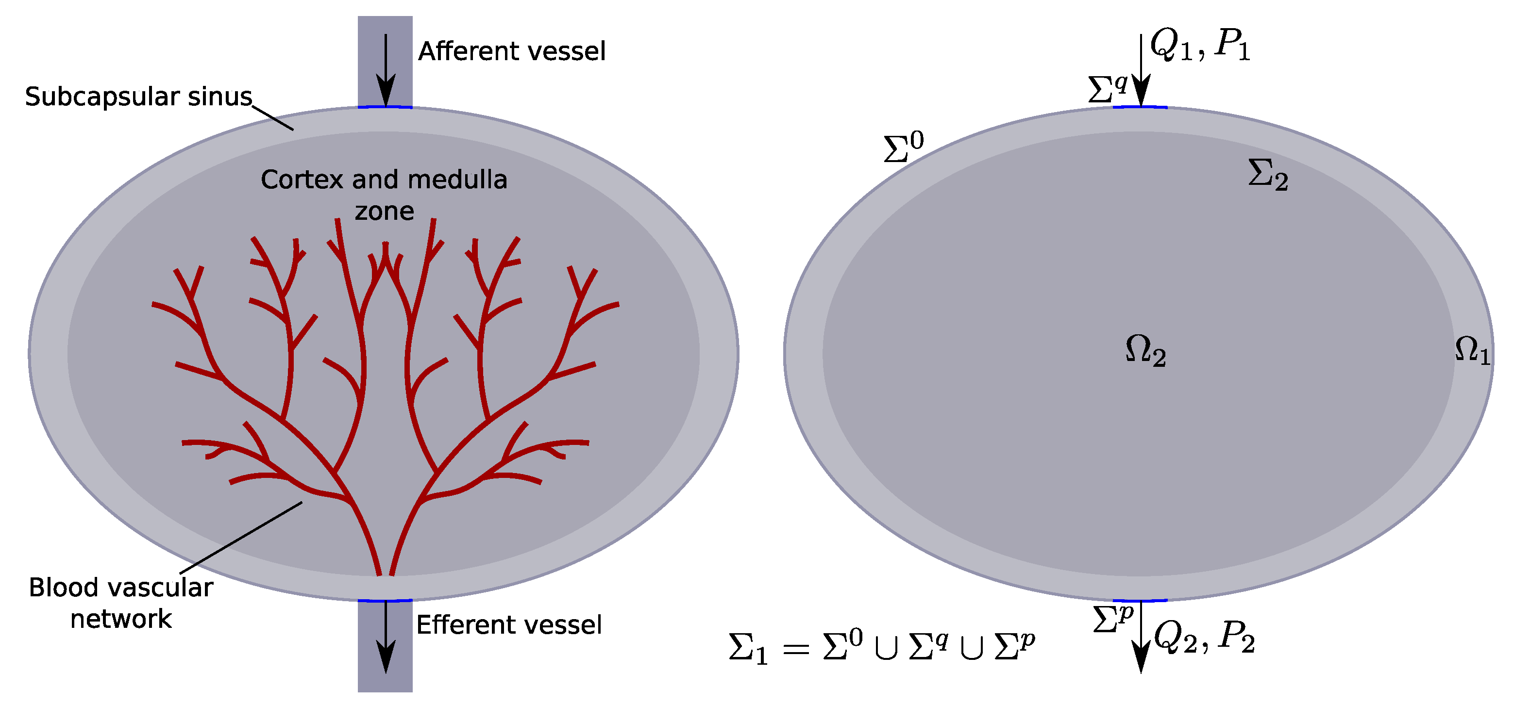
LNs have a variable appearance [38]. In an idealized case, their shape can be approximated by a sphere or an ellipsoid with diameters ranging from 0.5–1 mm to 30–50 mm and more [39]. Lymph nodes typically have 2–4 afferent (input) vessels and 1–2 efferent (output) vessels. Intraluminal valves of the vessels at the junctions of LNs and lymphatic vessels provide a unidirectional flow of lymph [39]. The spatial structure of an idealized LN considered in this study is represented by the set of two spatial domains: the external domain, i.e., the subcapsular sinus, and the internal one, constituted by the cortex area including the T-cell zone, B-cell follicles and the medullar zone (see Figure 1, left). The outer boundary of the external domain consist of non-permeable part ${\Sigma }_1$ and the lymphatic vessel–LN junctions ${\Sigma }_q$, ${\Sigma }_p$ (see Figure 1, right) through which the inflow and outflow of lymph takes place.

The two spatially distinct domains being filled with the immune cells are considered as homogeneous porous media, characterized by different hydraulic conductivity being constant in each domain. Therefore, it is assumed that in both of the considered LN domains, the lymph filtration can be described by Darcy’s law.

It is known that when lymph passes through the lymph node about one-third of its volume can be absorbed by LN blood vessels (BVs), which are present in the internal domain, into the CS [39]. The corresponding fluid exchange between the CS and LNs via BVs needs to be taken into account when building physics-based and NN-type models of the fluid flow through the LNs. The lymph exchange with the CS via BVs is modeled by Starling’s equation.

3. Mathematical Model of LN Drainage Function: Differential and Integral Forms

3.1. PDE-Based Model

We denote the whole computational domain as $\Omega ={\Omega }_1\bigcup {\Omega }_2$ which is bounded by a closed smooth surface ${\Sigma }_1$. ${\Sigma }_2$ is a boundary between the external domain ${\Omega }_1$ with higher hydraulic conductivity and the internal domain ${\Omega }_2$ with lower hydraulic conductivity. The computational domains corresponding to the simplified LN geometry are depicted in Figure 1, right.

The lymph is considered as homogeneous incompressible Newtonian fluid. Following previous studies [30,31], the lymph flow through the LN is described by Darcy’s law for the unknown fluid velocity $\mathit{v}$ and pressure p. In the external domain, the continuity equation is fulfilled, and in the internal domain, the lymph is exchanged with BVs according to Starling’s equation. The resulting system of PDEs reads:

$$\left\{\begin{array}{cc}\hfill & \mathit{v}\left(x\right)=-\frac{{\kappa }_i}{\mu }\nabla p\left(x\right)x\in {\Omega }_i,i=1,2,\hfill \\ \hfill & \nabla ·\mathit{v}\left(x\right)=0,x\in {\Omega }_1,\hfill \\ \hfill & \nabla ·\mathit{v}\left(x\right)=-L_{b}A(p\left(x\right)-p_b+\sigma ·\Delta \pi ),x\in {\Omega }_2.\hfill \end{array}\right.$$

(1)

The parameters of the model equations are: ${\kappa }_i$—the hydraulic conductivity of the domain ${\Omega }_i$, $i=1,2$, $\mu$—lymph dynamic viscosity, $L_b$—the average hydraulic conductivity of the blood vessel walls in the LN, A—the surface area of the blood vessels participating in the filtration of lymph, $p_b$—the average blood vessel pressure, $\Delta \pi$—the average difference of oncotic pressure between the blood vessels and the interior domain of the LN and $\sigma$—the oncotic reflection coefficient.

The outer boundary is divided into three parts: ${\Sigma }_1={\Sigma }^0\bigcup {\Sigma }^q\bigcup {\Sigma }^p$. These correspond to the afferent vessel–LN junction ${\Sigma }^q$ with a given lymph velocity, the efferent vessel–LN junction ${\Sigma }^p$ with a given pressure value and the impermeable outer boundary ${\Sigma }^0$ with no flux. The interface between the two domains ${\Sigma }_2$ is considered to be homogeneous, with the pressure and normal component of the velocity vector assumed to be continuous at this boundary. We denote the outer side of each surface ${\Sigma }_m$, $m=1,2$ as positive with $\mathit{n}\left(x\right)$, $x\in {\Sigma }_m$, $m=1,2$ being the unit vector orthogonal to surface ${\Sigma }_m$ at point x.

The boundary conditions are set as following:

$$\left\{\begin{array}{ccc}\hfill & \mathit{n}\left(x\right)·{\mathit{v}}^{-}\left(x\right)-\xi \left(x\right)=f_0\left(x\right),\hfill & \hfill x\in {\Sigma }_1;\\ \hfill & p^{-}\left(x\right)=\psi \left(x\right),\hfill & \hfill x\in {\Sigma }^p;\\ \hfill & \mathit{n}\left(x\right)·({\mathit{v}}^{+}\left(x\right)-{\mathit{v}}^{-}\left(x\right))=0,\hfill & \hfill x\in {\Sigma }_2;\\ \hfill & p^{+}\left(x\right)-p^{-}\left(x\right)=0,\hfill & \hfill x\in {\Sigma }_2.\end{array}\right.$$

(2)

Here, $f_0\left(x\right)$ is a given lymph flow velocity through the afferent vessel, $f_0\left(x\right)\equiv 0,x\notin {\Sigma }^q$. $\psi \left(x\right)$ is a given pressure on efferent vessel ${\Sigma }^p$. We also introduce an extra variable $\xi \left(x\right)$ equal to lymph flow velocity through efferent vessel ${\Sigma }^p$, $\xi \left(x\right)\equiv 0,x\notin {\Sigma }^p$.

3.2. Boundary Integral Equation-Based Model

For numerical modeling of lymph filtration flow in the LN we developed an equivalent representation of the above mathematical model using the boundary integral equations approach [40]. The model briefly described below is based on the results obtained in our previous work [41,42]. Similar to the PDE boundary value problem, at the afferent vessel–LN border, the lymph flow velocity is considered to be given, whereas at the efferent vessel–LN interface, the lymph pressure is specified. The lymph flow velocity and lymph pressure are represented as sums of integral operators specified at the outer and inner boundaries.

To reduce the number of the model parameters, we combine some of the parameters as follows:

$${\alpha }_i=\frac{\mu }{{\kappa }_i},L=L_{b}A,P_v=p_b-\sigma ·\Delta \pi .$$

(3)

The velocity vector field can be considered as the gradient of some potential function, i.e., $\mathit{v}=\nabla \phi$, with the potential $\phi$ being proportional to pressure $\phi =-p/{\alpha }_i$ in each domain ${\Omega }_i$, $i=1,2$. Following the approach presented in [41,42], we express the velocity and pressure fields in domains ${\Omega }_1$, ${\Omega }_2$ as sums of the boundary integrals:

$$\begin{array}{cc}\hfill & \mathit{v}=\nabla W_{{\lambda }_i}[{\Sigma }_1,h]+\nabla U_{{\lambda }_i}[{\Sigma }_2,g]+\nabla W_{{\lambda }_i}[{\Sigma }_2,h],\hfill \\ \hfill & p=-{\alpha }_i\left(W_{{\lambda }_i}[{\Sigma }_1,h]+U_{{\lambda }_i}[{\Sigma }_2,g]+W_{{\lambda }_i}[{\Sigma }_2,h]\right)+{\chi }_{{\Omega }_2}{p}_v.\hfill \end{array}$$

(4)

Here, ${\lambda }_1=0$ in ${\Omega }_1$ and ${\lambda }_2=\sqrt{L{\alpha }_2}$ in ${\Omega }_2$, ${\chi }_{{\Omega }_2}$ are the domain indicator functions for ${\Omega }_2$.

The following integral operators are used to construct the solution: $W_{\lambda }[S,h]$ is the potential of a simple layer, with density h, $U_{\lambda }[S,g]$ as the double layer potential with density g:

$$\begin{array}{cc}& W_{\lambda }[S,h]\left(x\right)={\int }_{S}h\left(y\right)F_{\lambda }(x-y)d{\sigma }_y,\hfill \\ & U_{\lambda }[S,g]\left(x\right)={\int }_{S}g\left(y\right)\frac{\partial F_{\lambda }(x-y)}{\partial n_y}d{\sigma }_y,\hfill \end{array}{F}_{\lambda }(x-y)=\frac{e^{-\lambda |x-y|}}{4\pi |x-y|}.$$

The divergence of the flow velocity vector is zero in ${\Omega }_1$: $\nabla ·\mathit{v}=0$, and consequently $\Delta \phi =0$, so $\phi$ is the Laplace’s potential in ${\Omega }_1$. Simple layer potential $W_0[{\Sigma }_1,h]$ with density h satisfies Laplace’s equation.

Potential $\phi$ in ${\Omega }_2$ is a solution of inhomogeneous Helmholtz’s equation:

$$\Delta \phi -{\lambda }^2\phi ={\lambda }^2\frac{P_v}{{\alpha }_2},{\lambda }^2=L{\alpha }_2.$$

Its solution is the sum of a particular solution of the inhomogeneous equation ${\phi }_v=-P_v/{\alpha }_2$ and of the general solution of the homogeneous equation. In turn, the general solution is expressed as the sum of the simple layer and the double layer potentials $W_{\lambda }[{\Sigma }_2,h]$, $U_{\lambda }[{\Sigma }_2,g]$.

Thus, the velocity and pressure fields in the form (4) satisfy the PDE system (1). Following the approach developed in papers [41,42], the solution (4) is substituted in the boundary conditions system (2), giving rise to the system of integral equations for the unknown potential densities of a simple and double layer h, g. The system is solved by the numerical method developed in [42].

In the next section, we specify physiologically plausible ranges and the probability distribution functions for the model parameters.

4. Physiological Variability of Model Parameters

The physics-based model (1)–(2) provides a mechanistic description of the LN filtering/drainage function characteristics. The model can further be used to identify the relationships between the geometry and conductivity parameters and the input/output lymph flow properties by applying the machine learning approach. The corresponding mapping function between the input parameters and the emergent properties of the LN function can be approximated by training a neural network (NN)-type model. The resulting NN-based emulator complements the mechanistic model and provides a computationally efficient tool to rapidly compute the parameters of the LN function, e.g., in a sensitivity analysis of the LN performance. To teach the NN, a training dataset needs to be generated using the mechanistic model with the parameters of the boundary value problem (1)–(2) varying within their physiological ranges. To estimate the ranges of the respective parameters, we used the experimental data as described below.

One group of parameters specifies the geometry characteristics of an idealized LN. It is considered to be a solid object consisting of porous domains with its shape approximated by two embedded ellipsoids with a common center. This shape is selected to mimic the appearance of the inguinal LN of a naive adult mouse [43]. The external ellipsoid with its surface ${\Sigma }_1$ has radii $R_x=R_z=0.35$ mm, $R_y=0.5$ mm. The internal ellipsoid with the interface surface ${\Sigma }_2$ has radii $R_x=R_z=0.315$ mm, $R_y=0.45$ mm. The afferent and efferent lymphatic vessels are considered to be cylindrical with the radius $r_0=0.075$ mm and the centers specified by coordinates $x_{in}$ and $x_{out}$ being located on the upper and bottom poles of ${\Sigma }_1$, respectively.

To characterize the functional properties of the LN, we consider the following parameters:

• $Q_1$—the rate of lymph flow into the LN through an afferent vessel;
• $Q_2$—the rate of lymph flow out of the LN via an efferent vessel;
• $Q_v$—the rate of lymph exchange with the lymph node BVs;
• $P_1$—the fluid pressure at the afferent lymphatic vessel;
• $P_2$—the fluid pressure at the efferent lymphatic vessel.

We divide the model parameters into two groups, i.e., those which can be quantified directly using the available experimental data and the parameters which need to be estimated by data fitting.

4.1. Experimentally Quantified Parameters

The following parameters determining the boundary conditions are directly accessible from experimental studies in [35]: $Q_1$, $P_2$, $p_b$, $\Delta \pi$ and $\sigma$. In brief, the studies were performed to examine the dependence of fluid transfer through the dog’s popliteal lymph node and the protein concentration of the efferent lymph fluid on the efferent lymphatic pressure. The isolated dog popliteal nodes of six dogs were used. The lymph, having a protein concentration averaging $27.6\pm 1.2\%$ (SD) of that of plasma, was infused into the node at a flow rate averaging $45.6\pm 0.2$ (SD) $\mathsf{\mu }$L/min. The efferent flow, afferent pressure and protein concentration efferent flow were measured. Overall, there are 38 data points in

Table 1. Experimental estimates for model parameters determining the boundary conditions: average value, minimal and maximal values and the assumed probability distribution function (based on experimental data from [35]).

Parameter	Measurement	Avg. Value	Min. Value	Max. Value	Distribution
$Q_1$	$\mathsf{\mu }$L/min	45.5	45.0	46.5	Uniform
$P_2$	mmHg	7	1	13	Uniform
$p_b$	mmHg	8.0	6	20.5	Triangular
$\Delta \pi$	mmHg	12.7	10.7	14.9	Triangular
$\sigma$	–	0.88	0.8	0.9	Uniform

from [35] (6–7 measurements per animal). We used 32 data points that remained after we discarded 6 measurements for which non-physiological efferent lymph pressures were used in the experiments.

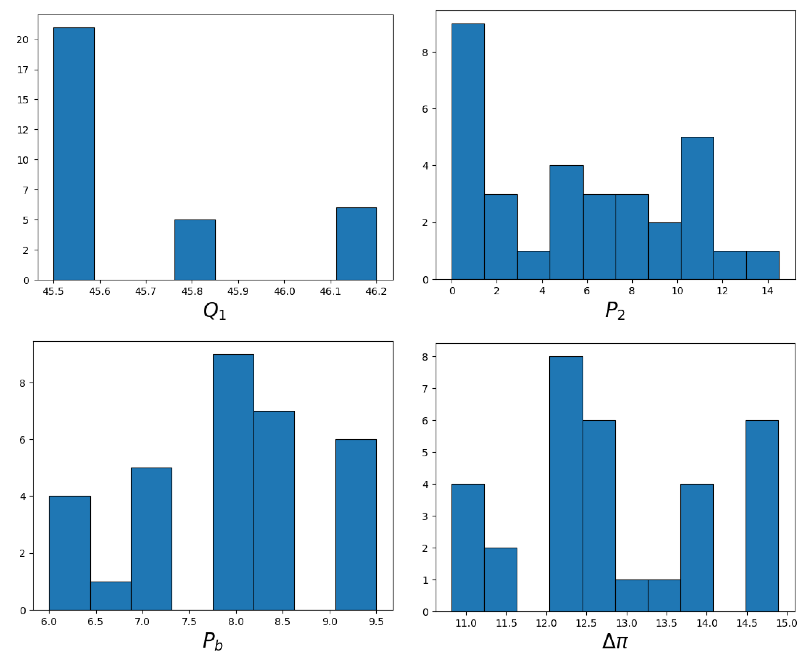
In the experiments, the afferent flow $Q_1$ was kept constant taking one of three different values (Figure 2). Hence, we assume that $Q_1$ is uniformly distributed over a range that covers the specified values. The efferent lymphatic pressure $P_2$ was another parameter being varied in all of the experiments with a peak frequency at $P_2=0$ (Figure 2). The probability distribution of the efferent lymphatic pressure $P_2$ is also assumed to be uniform. For the parameters $p_b$ and $\Delta \pi$ (shown in Figure 2), a triangular distribution is assumed. The oncotic reflection coefficient $\sigma$, as indicated in [30,31], takes values from 0.8 to 0.9. For it, a uniform distribution is assumed. Overall, the available experimental data provide the following estimates of the physiological ranges for parameters $Q_1$, $P_2$, $p_b$, $\Delta \pi$ and $\sigma$ summarized in Table 1.

As the lymph flow is considered to be laminar and Newtonian, the flow velocity profile is parabolic. The boundary conditions of system (1)–(2) are functions $f_0$, $\psi$ and parameter $P_v$, which depends on $p_b$, $\Delta \pi$ and $\sigma$. The functions $f_0$ and $\psi$ are expressed via $Q_1$ and $P_2$ as follows:

$$\begin{array}{cc}\hfill & f_0\left(x\right)=-Q_1\frac{r_0^2-{|x-x_{in}|}^2}{S_1},x\in {\Sigma }^q,S_1={\int }_{{\Sigma }^q}(r_0^2-|x-x_{in}{|}^2)d\sigma ;\hfill \\ \hfill & \psi \left(x\right)=P_2,x\in {\Sigma }^p.\hfill \end{array}$$

(5)

4.2. Estimated Parameters

The governing Equations (1)–(2) contain the physics-defined parameters L, ${\alpha }_1$ and ${\alpha }_2$. They depend on physiological characteristics of LN: ${\kappa }_1$, ${\kappa }_2$, $\mu$, $L_b$ and A as described by (3). Specifically, the parameters ${\alpha }_i=\mu /{\kappa }_i$, $i=1,2$ and ${\alpha }_2>{\alpha }_1$ characterize hydraulic resistances of the corresponding porous media, whereas $L=L_{b}A$ defines the rate of absorption of lymph into lymph node BVs.

To evaluate the physiologically plausible ranges of the above parameters, we examined the characteristics of simulations of lymph flow through the LN for various values of the parameters. The square cuboid is the model parameter space for which the model solutions reproduce the following scenarios: (1) the lymph absorption by BVs ranges from zero to $Q_1$, and (2) the flow resistance of the external domain ($S_1$) increase from 0 to ∞. The model predicts the following physiologically relevant ranges of the parameter to be estimated:

• For $L<{10}^{-1}$, the absorption is minimal: $Q_v\to 0$;
• For $L>{10}^2$, the absorption is maximal: $Q_v\to Q_1$;
• For ${\alpha }_1<{10}^{-5}$, the lymph flow experiences no resistance: $P_1\to P_2$;
• For ${\alpha }_1>{10}^{-2}$, the required pressure difference ($P_1-P_2$) to keep the flow (to overcome the resistance) increases: $P_1\to \infty$;
• For ${\alpha }_2<{10}^{-4}$, the absorption is maximal: $Q_v\to Q_1$;
• For ${\alpha }_2>{10}^2$, the absorption is minimal: $Q_v\to 0$.

The resulting domain in the parameter space is given by the following square cuboid $R{C}_3=[{10}^{-1},{10}^2]\times [{10}^{-5},{10}^{-2}]\times [{10}^{-4},{10}^2]$.

The experimental data [35] allow us to quantify the uncertainty ranges for the parameters $L,{\alpha }_1,{\alpha }_2$ following the procedure described below:

• Randomly sample the value $\theta =\{L,{\alpha }_1,{\alpha }_2\}$ from $R{C}_3$;
• Compute the solution of the boundary integral equations system modeling the LN function;
• Check the consistency of the model-predicted values of $Q_2^i$, $P_1^i$ and the experimental data for $i=1,N_{exp}$;
• Update the uncertainty interval $R{C}_3$ to get the data-based square cuboid $R{C}_{3,fitted}$.

In addition, the best-fit model parameters were estimated by minimizing the mismatch error functional ${\Phi }_{err}\left(\theta \right)$.

$${\Phi }_{err}\left(\theta \right)={\left(\sum _{i=1}^{N_{exp}}\frac{{(Q_2^i-{\overline{Q}}_2^i\left(\theta \right))}^2}{{\left(Q_2^i\right)}^2}+\frac{{(P_1^i-{\overline{P}}_1^i\left(\theta \right))}^2}{{\left(P_1^i\right)}^2}\right)}^{\frac{1}{2}}.$$

(6)

The permissible ranges for the model parameters L, ${\alpha }_1$, ${\alpha }_2$ are given in

Table 2. Estimated model parameters: notation, units, best-fit value giving a minimium of the functional ${\Phi }_{err}\left(\theta \right)$ (6) and plausible intervals of parameter values.

Parameter	Measurement	Optimal Value	Interval	Distribution
L	(mmHg·min)${}^{-1}$	8	[1, 20]	Normal
${\alpha }_1$	mmHg·min/mm${}^2$	$2.2\times {10}^{-3}$	$[1\times {10}^{-4},4\times {10}^{-3}]$	Normal
${\alpha }_2$	mmHg·min/mm${}^2$	2.2	[0.1, 10]	Uniform

.

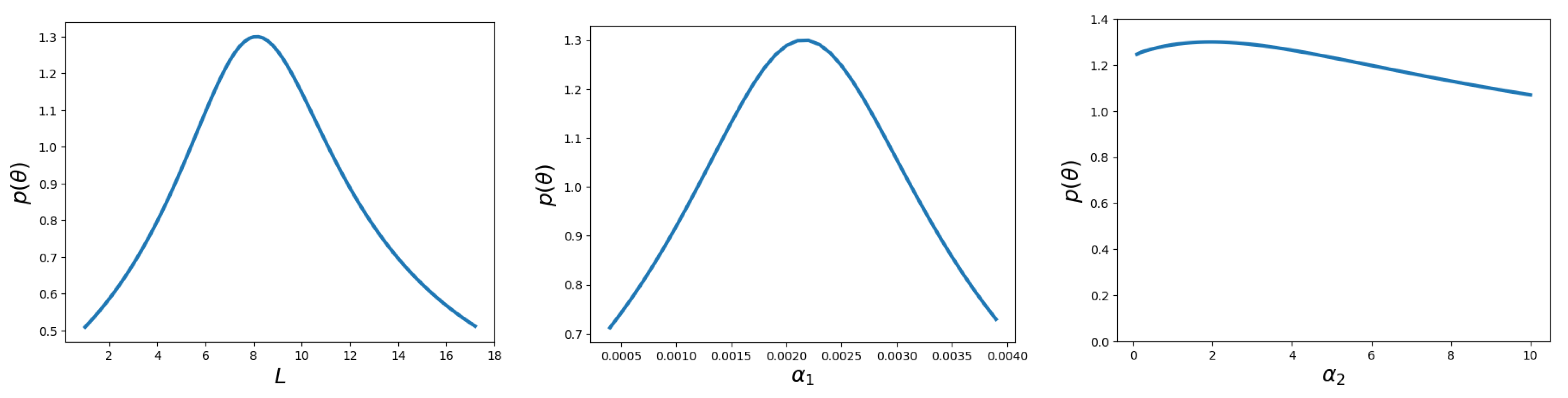
The inverse of the functional

$$p\left(\theta \right)=\frac{1}{{\Phi }_{err}\left(\theta \right)}.$$

(7)

We used as a surrogate of the likelihood function to qualitatively infer the probability distribution of the estimated model parameters. The cross-sections of the functions $p\left(\theta \right)$ for each parameter are shown in Figure 3.

5. Neural Network Model of Lymph Node Drainage Function

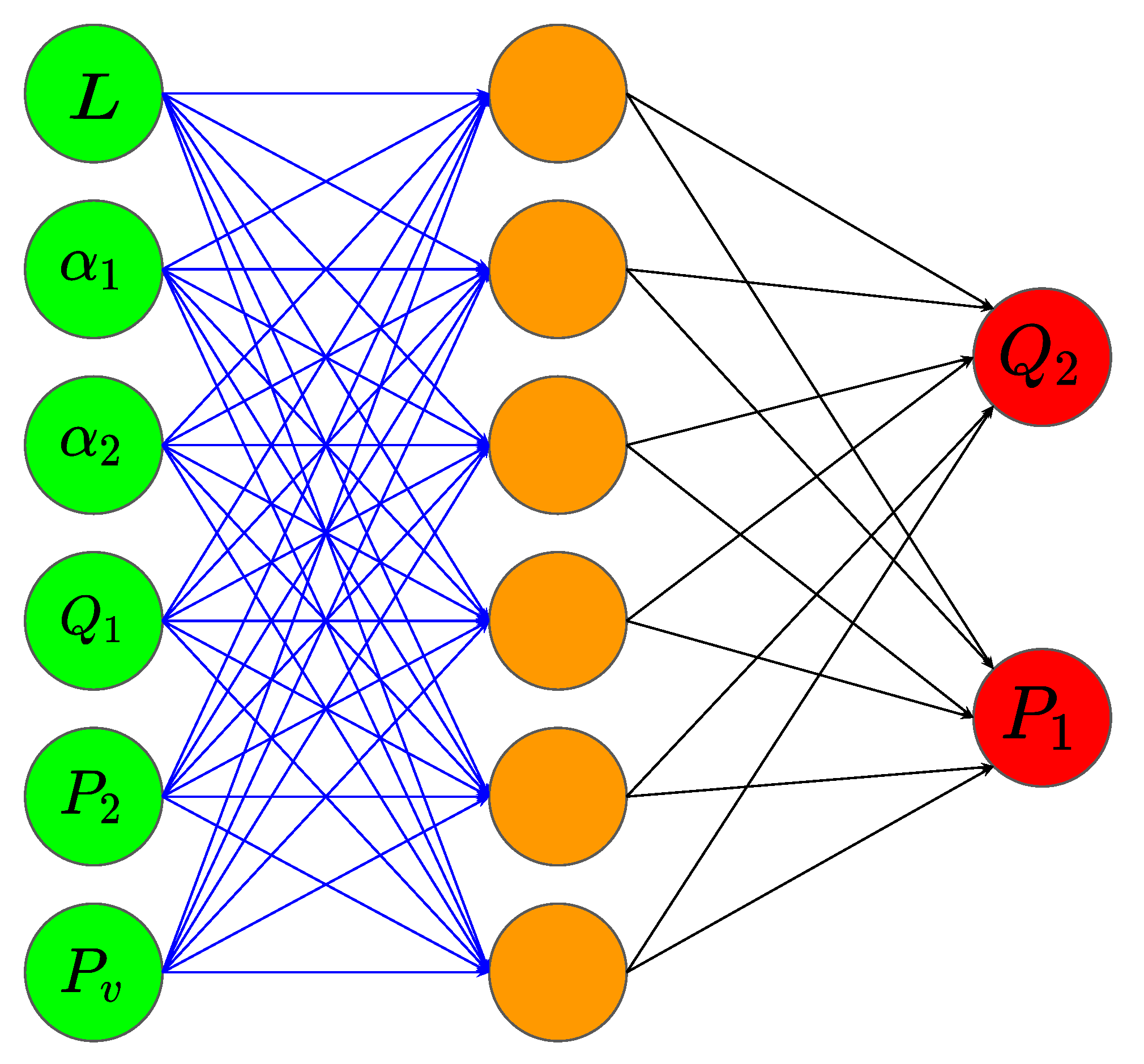
We develop a feedforward neural network to emulate the filtering function of the LN. This type of NN model consists of an input layer, A few hidden layers and an output layer. The development of the NN model requires the following steps: preparation of the data (simulation-based generation), training of the neural network model and testing of its performance. The input layer of the neural network consists of six nodes corresponding to the following parameters of the model: $Q_1$, $P_2$, $P_v$, L, ${\alpha }_1$, ${\alpha }_2$. The output layer of the NN consists of two nodes specifying the elements to be quantitatively predicted: the efferent lymph flow $Q_2$ and the afferent pressure $P_1$. The amount of lymph absorbed into the lymph node BVs is $Q_v=Q_1-Q_2$.

5.1. Generation of Training Dataset

For optimal sampling of the parameters, we use the Latin hypercube sampling (LHS) method. The algorithm for constructing an optimal sample of parameters is as follows.

• For each parameter ${\theta }_i$, $i=1,...,M$, we set permissible ranges $[a_i,b_i]$ and the function $p_i\left(x\right)$ as the model probability density (see Table 1 and Table 2).
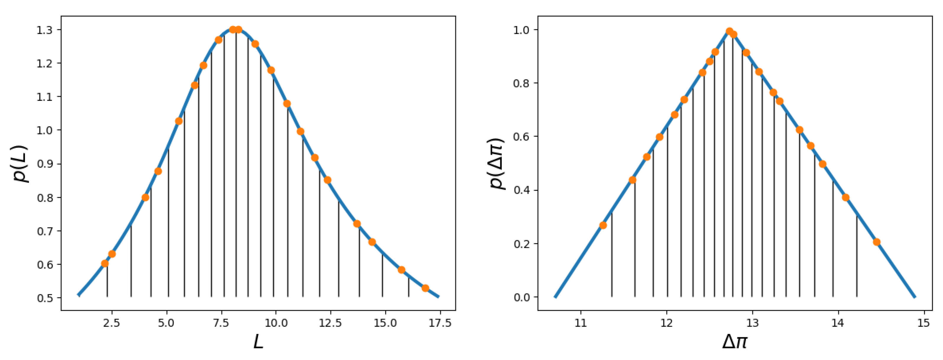
• Segment $[a_i,b_i]$ is divided into N equiprobable segments, one random point $x_{ij}$, $j=1,N$ is taken on each segment as shown in Figure 4.
• For each parameter ${\theta }_i$, the set of its values $x_{ij}$ is randomly shuffled (by index j).
• The training sample of parameters consists of the J sets $x_{ij}$ ($i=1,...,M$, $j=1,...,J$).

The parameter sets generated by the algorithm given above are used to calculate the efferent lymph flow $Q_2$ and the afferent lymph pressure $P_1$ by simulations of the boundary integral equations model. Note that for evaluation of the composite parameter $P_v$, appearing in the integral equations-based model and the NN model, the sampled values of three parameters $P_b$, $\Delta \pi$, $\sigma$ were used.

5.2. Construction of Neural Network Model

Overall, 200 combinations of parameters $L,{\alpha }_1,{\alpha }_2,Q_1,P_2,P_v$ were generated by the LHS method. Using the integral equations model of the lymph flow through the LN (see Section 2), we calculated the output values $Q_2,P_1$ for each combination of the input parameters. Thus, we obtained two datasets for (1) training and (2) validation of the NN model (with 1:1 split ratio).

The architecture of the NN model is shown in Figure 5. It is a fully connected neural network containing one hidden layer consisting of six neurons (nodes). The sigmoid activation function was used for the hidden layer neurons. The output values were determined by a linear combination of the values in the hidden layer nodes. Let us designate $\mathit{x}={(L,{\alpha }_1,{\alpha }_2,Q_1,P_2,P_v)}^T$ as the input vector, ${\mathit{x}}_{\mathit{h}}$—the state vector of hidden layer neurons and $\mathit{y}={(Q_2,P_1)}^T$—the output vector. The values in the hidden layer and in the output are calculated using the following equations:

$$\left\{\begin{array}{cc}\hfill & {\mathit{x}}_{\mathit{h}}=\mathit{\xi }\left({\mathit{W}}_{\mathbf{1}}\frac{\mathit{x}-{\mathit{a}}_{\mathbf{1}}}{{\mathit{a}}_{\mathbf{2}}}+{\mathit{b}}_{\mathbf{1}}\right),\mathit{\xi }\left(\mathit{x}\right)=\frac{1}{1+e^{-\mathit{x}}}\hfill \\ \hfill & \mathit{y}={\mathit{W}}_{\mathbf{2}}{\mathit{x}}_{\mathit{h}}+{\mathit{b}}_{\mathbf{2}},\hfill \end{array}\right.$$

(8)

with ${\mathit{W}}_{\mathbf{1}}$ and ${\mathit{W}}_{\mathbf{2}}$ being weight matrices, ${\mathit{b}}_{\mathbf{1}}$ and ${\mathit{b}}_{\mathbf{2}}$ are bias vectors, $\mathit{\xi }\left(\mathit{x}\right)$ is vector-function and ${\mathit{a}}_{\mathbf{1}}$ and ${\mathit{a}}_{\mathbf{2}}$ are vectors of normalization coefficients. $\mathit{\xi }\left(\mathit{x}\right)$ is a notation for vectorized operation, i.e., this operation is performed over every element of the array (x). The algorithm presented in the Fast Artificial Neural Network (FANN) library [44] (implemented in C++ language) was applied to train the model (implemented in C++ language). The training was performed using the error backpropagation method. The trained values of ${\mathit{W}}_{\mathbf{1}}$, ${\mathit{W}}_{\mathbf{2}}$, ${\mathit{a}}_{\mathbf{1}}$, ${\mathit{a}}_{\mathbf{2}}$, ${\mathit{b}}_{\mathbf{1}}$ and ${\mathit{b}}_{\mathbf{2}}$ are given in Appendix A.

In addition, the training dataset was used to identify a statistical model, i.e., a linear regression (LR) of $\mathit{y}$ on covariates $\mathit{x}={(L,{\alpha }_1,{\alpha }_2,Q_1,P_2,P_v)}^T$. The output (response) variables were described by the following regression equation $\mathit{y}={\mathit{W}}_{\mathbf{3}}\frac{\mathit{x}-{\mathit{a}}_{\mathbf{1}}}{{\mathit{a}}_{\mathbf{2}}}+{\mathit{b}}_{\mathbf{3}}$, with the weight matrix ${\mathit{W}}_{\mathbf{3}}$, and bias vector ${\mathit{b}}_{\mathbf{3}}$ (the values of elements of ${\mathit{W}}_{\mathbf{3}}$ and ${\mathit{b}}_{\mathbf{3}}$ are given in Appendix A).

Note that we experimented with a large number of hidden layers and the number of neurons in these layers, but the result was not significantly better than the one presented in the article. We did not consider alternative neural network architectures in terms of the principles of organizing the connections between layers, but only used a classical network with direct signal propagation from inputs to outputs. This is consistent with the functionality of the FANN library we used. For NN models with more than one hidden layer, the accuracy of the models on the validation dataset did not improve.

6. Validation of the Neural Network Model

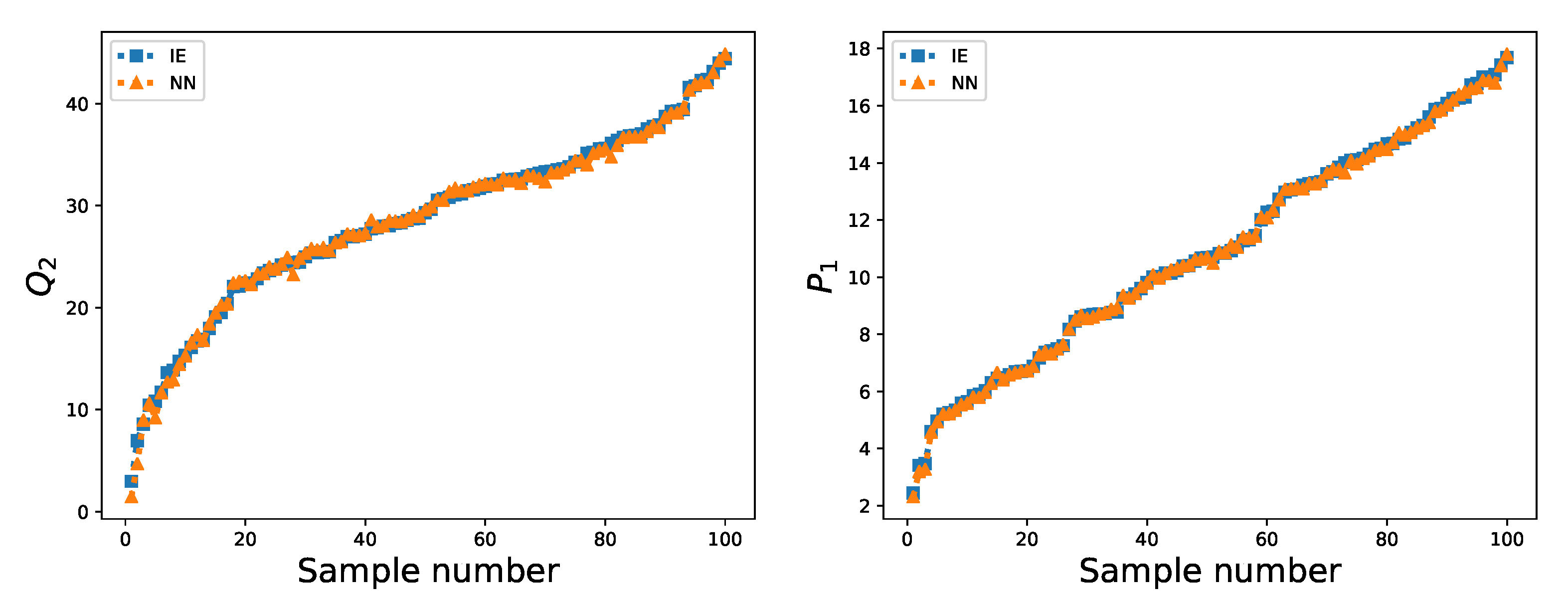
To test the NN model performance, the validation dataset (100 simulations) was used. Figure 6 shows the validation set output values $Q_2$, $P_1$ of the integral equations model and the predictions of the trained NN model. The values of the output variables are ranked in ascending order.

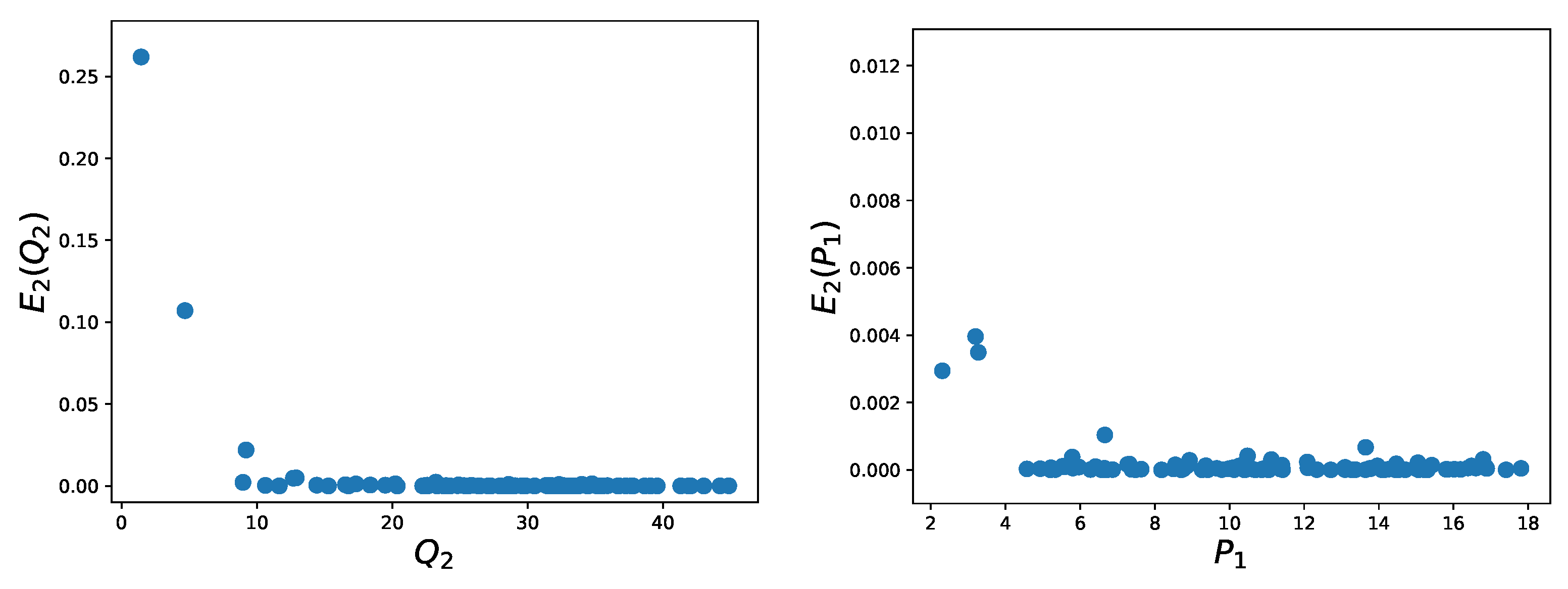
To characterize the accuracy of the NN predictions, the quadratic error functional $E_2$ and the logarithm error functional $E_{lg}$ were estimated. These functionals evaluate the relative error as follows:

$$E_2=\frac{{(X_{IE}-X_{NN})}^2}{X_{IE}^2},E_{lg}=-10lg\left(E_2\right).$$

(9)

Here, $X_{NN}$ stands for one of the integral equations model outputs $Q_2$ or $P_1$, whereas $X_{NN}$ is the corresponding NN model prediction. Figure 7 presents the estimated prediction error on the validation dataset. The average and the maximum values of the error for the NN and LR models are detailed in

Table 3. Mean and maximum values of the relative error functional (9) for the neural network and linear regression models.

	X	$max\left({\mathit{E}}_2\right)$	mean$\left({\mathit{E}}_2\right)$	$min\left({\mathit{E}}_{\mathit{lg}}\right)$	mean$\left({\mathit{E}}_{\mathit{lg}}\right)$
Neural network	$Q_2$	0.22	$4\times {10}^{-3}$	6.5	43.1
Linear regression	$Q_2$	5.4	$7\times {10}^{-2}$	−7	27.5
Neural network	$P_1$	$1\times {10}^{-2}$	$2\times {10}^{-4}$	20.2	47.5
Linear regression	$P_1$	$3.6\times {10}^{-2}$	$1\times {10}^{-3}$	14.5	38.2

.

The NN model performs with the relative accuracy of about ${10}^{-3}$. The linear regression model performance is characterized by the mean prediction error of about ${10}^{-1}$. The accuracy of predicted $Q_2$ is much lower than that of $P_1$. Hence, one can conclude that the lymph filtration in the LN described by the systems of Equations (1) and (2) is a physical process with a non-linear dependence on the parameters of the governing equations and of the boundary conditions. The emerging non-linearity in the lymph flow behavior underlies the poorer prediction of the validation dataset demonstrated by the LR model.

To further test the predictive quality of the NN model, we considered the experimental dataset (Table 1 data in [35]). The data present the experimental results for six animals with six to seven measurements per animal. Overall, 32 data points were considered after the removal of 6 measurements for which non-physiological efferent lymph pressures were used in the experiments. For each animal, we evaluated the best-fit values of parameters $\theta$ by minimizing the functional ${\Phi }_{err}\left(\theta \right)$, specified in (6), using the Nelder–Mead method. The optimal estimates of the model parameters combined with the experimental data were used as the input parameters of the NN model. The predicted output values $Q_2$, $P_1$ were compared with the experimental results. Figure 8 presents the values $Q_2$ and $P_1$ predicted the by NN and IE models versus the results of the experiments. Overall, the predictions of the NN model are similar to the results of the IE model, except for two points with the highest values of $Q_2$. However, both models display some deviations from the experimental data noticeable for small values of $P_1$. Taking into account that the mismatch characterized by the error metrics are comparable with the accuracy of the experimental data, i.e., max$\left(E_2\left(Q_2\right)\right)=0.02$, max$\left(E_2\left(P_1\right)\right)=0.4$, mean$\left(E_2\left(Q_2\right)\right)=0.002$ and mean$\left(E_2\left(P_1\right)\right)=0.08$, the deviations at the lower end of the afferent lymph pressure can be considered as acceptable.

One of the major advantages of the developed NN model is the computation time required for predicting the characteristics of the drainage function. Indeed, the NN training on 100 datasets requires about 20 s of CPU time. The computation of $Q_2$ and $P_1$ for 100 parameter samples by the trained NN takes about ${10}^{-4}$ s. In contrast, the computation time for 100 realizations of the integral equation-based mathematical model requires about 7.8 h.

7. Conclusions

We have developed an artificial neural network model to describe the lymph node drainage function. The NN model predicts the flow characteristics through the LN, including the exchange with the blood vascular system in relation to the boundary and lymphodynamic conditions, such as the afferent lymph flow, Darcy’s law constants and Starling’s equation parameters. The model has been formulated as a feedforward NN with one hidden layer. The NN complements the computational physics-based model of a stationary fluid flow through the LN and the fluid transport across the blood vessel system of the LN. The physical model is specified as a system of boundary integral equations equivalent to the original PDEs (Darcy’s Law and Starling’s equation) formulations [30,31]. To set up the model, we have considered a simplified LN geometry as consisting of two embedded 3D ellipsoids. The IEs model has been calibrated using the available set of classical physiological data on lymph filtration in the LNs [33,34,35]. The IEs model has been used to generate the training dataset for identifying the NN model architecture and parameters. The computation of the output LN drainage function characteristics (the fluid flow parameters and the exchange with blood) with the trained NN model required about 1000-fold less CPU time than computationally tracing the flow characteristics of interest with the physics-based IEs model.

The experimental data from [35] describes the dependence of fluid transfer characteristics through the dogs’ popliteal lymph nodes on the efferent lymphatic pressure. Totally, there are 38 data points for 6 dogs with 6–7 measurements per animal. The number of experimental data points is not sufficient for neural network training, so we did not train and validate the NN-based model directly on them. Instead, we used these data to estimate the physiological ranges and plausible distributions of IE-based model parameters (see Table 1 and Table 2 and Figure 3), as described in Section 4.1 and Section 4.2. Next, we synthesized the data using the IE-based model by sampling the model parameters from the determined distributions with Latin hypercube sampling (Section 5.1). We used the simulation-based data (200 points) to further train the NN-based (and regression-based) models. The synthetic data was split for training and validation of the NN-based model into two sets with 100 points in each set (Section 5.2). Finally, the experimental points were additionally used to validate the developed IE- and NN-based models (Figure 8).

The lymphatic system serves an important transport function in the human body and the body’s immune system [32]. The mathematical models of the LS developed so far describe various aspects of the system topology [8,9,10] and the lymph flow through lymphatic vessels [8,37,45]. The filtering function of the LNs has been much less explored [46] with some studies addressing the flow through the macroscopic structures [30,31] and the microscopic components, such as the conduit system [29,47]. In the available computational models of the whole LS [6,8], the lymph nodes are treated as a type of lymphatic vessel. However, the LNs are the key structures of the LS where the fluid exchange with the blood vascular system takes place. The volume of the exchanged fluid is determined by the following LN characteristics represented in the model: the hydraulic conductivity of the porous medium, the total surface area of blood vessels, the hydraulic conductivity of BV walls, the afferent lymph flow rate, the efferent lymph and blood pressure and the difference in oncotic pressures of blood and lymph. Whereas the integration of the physics-based models [30,31] of the LN into the whole LS in silico models remains to be computationally challenging, the use of the NN model with its ability to promptly compute the lymph balance parameters in the LN for some given lymph inflow characteristics and the parameters of the porous media mimicking the hydraulic LN properties makes it an appropriate tool for integration with the systemic lymphodynamics description.

The lymphatic system has a highly variable structure [7] with about 450 LNs in humans [48]. In turn, the architecture of the LN presents a variety of appearances with differences in the numbers of afferent and efferent lymphatic vessels and shapes of the macrostructures (e.g., subcapsular sinuses, lymphoid lobules and the surface area of the blood capillary network). In our study, a simplified geometric model of the LN was considered. The developed approach to modeling LN drainage function utilizing a combination of a physics-based model and a neural network-type model can be adapted to the LN with an arbitrary shape and afferent/efferent vessels in a number of locations. To this end, one would need to define a set of physiologically observed and structurally distinct LNs and generate the integral equation-based and NN models linking the input parameters to the characteristics of the drainage function of interest, subject to the availability of the calibration dataset. The elements of the computational LN models library could be assembled into a personalized virtual LS description by embedding them into a graph model of the LS maximally reflecting the available data on an individual’s LN shapes, sizes and number as well as the LS topology.

The presented approach to constructing a NN-type model describing lymph node drainage function can be tailored for more complex lymph node architecture. For example, the simplified geometric model of the LN can be refined to include more macroscopic structures, such as afferent and efferent lymphatic vessels, the B-cell follicles and trabecular and medullar sinuses. The complexity of the LN geometry and shortage of experimental data on the hydrodynamics properties of live LNs makes modeling the LN filtering function a challenging task. In summary, we developed an artificial neural network model of the lymph flow through the LN and fluid exchange with blood vessels in the LN. Comparing the performance of NN model with the statistical regression on the simulated data generated with the physics-model which display a non-linear behavior, we conclude that the accuracy of the NN model is superior.

LNs are the sites where the composition of the incoming lymph fluid is modified [26]. Lymph is composed of soluble proteins, pre-processed antigens, metabolites, exosomes as well as chemokines and cytokines [49]. Lymph-borne soluble factors flowing through the LN parenchyma have a direct impact on the structure, mechanical and transport properties of the LNs. Experimentally, it was shown that the amount of fluid exchange through the blood vessel walls can be modulated in either direction by changing the lymphatic hydrostatic and oncotic pressures [32,33]. The variation of the composition of incoming blood can be taken into account in our modeling approach by adjusting the oncotic pressure parameter $\Delta \pi$. Hence, its effect on the LN drainage function can be predicted with the NN model. The applicability of the model to predict the effects for broader contexts (cancer, aging, infections etc.) depends heavily on its calibration using the appropriate experimental data. The availability of quantitative data linking the lymph composition and lymphatic transport in the LN for clearly defined physiological contexts still remains to be a bottleneck [32,49].

Living organisms are characterized by an extremely complex and highly dimensional network of biochemical reactions that regulate the realm of the organism’s physiological functions, including the lymphatic transport through the LN. The filtering processes described in the developed computational model depend on the oncotic pressure, the porosity of the LN parenchyma and the permeability/area of the blood vessels walls. The impact of biochemical reactions within the LN can be taken into account either by parameterization of their effects on the respective model parameters or extending the model by considering the reaction kinetics explicitly. However, this would require a major shift in the complexity of the model to take into account the inflammatory processes and the formation of concentration gradients regulating the spatiotemporal dynamics of immune and stromal cells, which can be a subject of future research requiring multidisciplinary modeling efforts [50,51,52].

As multiscale approaches to modeling the immune system and infectious disease become mainstream in mathematical immunology, our study suggests efficient computational tools for the prediction of:

• The flow velocity patterns in the LN, determining the cytokine gradients and the cell migration, for which the physics-based boundary integral equations model can be used;
• The bulk fluid exchange between the LN parenchyma and the HEVs, for which the NN model provides a prompt solution.

These will allow a more realistic description and prediction of the immune cell circulation, cytokine distribution and drug pharmacokinetics in humans under various health and disease states as well as assisting in the development of artificial LN-on-a-chip technologies [52].

It is established that certain pathological conditions in humans (e.g., cancer metastasis, HIV-induced dysfunction and poor vaccine responses) are associated with perfusion defects in respective (e.g., sentinel or draining) LNs [53,54,55]. The underlying processes include the changes in the density of cells, the angiogenesis and the collagen deposition. A hypothesis on perfusion defect could be linked to the alteration in surface area of the LN blood vessels participating in the filtration of lymph, the hydraulic conductivity of the cortex area, abnormal hemodynamics in neovascular vessels, etc. All of them are represented in the model by their respective parameters and their quantitative alterations can be estimated from the ultrasound, CT or MRI image data using the modeling tools developed in our study. Hence, the approach can be applied to quantify certain parameters of LN drainage function to better understand the mechanisms and the plausible causes of the observed deviations of lymph transport through the LN and to make informed decisions on the appropriate treatments.

References

- Hunter, P.J.; Borg, T.K. Integration from proteins to organs: The Physiome Project. Nat. Rev. Mol. Cell Biol. 2003, 4, 237–243. [Google Scholar] [CrossRef]
- Randolph, G.J.; Ivanov, S.; Zinselmeyer, B.H.; Scallan, J.P. The Lymphatic System: Integral Roles in Immunity. Annu. Rev. Immunol. 2017, 35, 31–52. [Google Scholar] [CrossRef] [PubMed] [Green Version]
- Moore, J.E., Jr.; Bertram, C.D. Lymphatic System Flows. Annu. Rev. Fluid Mech. 2018, 50, 459–482. [Google Scholar] [CrossRef]
- Hruby, R.J.; Martinez, E.S. The Lymphatic System: An Osteopathic Review. Cureus 2021, 13, e16448. [Google Scholar] [CrossRef]
- Liao, S.; von der Weid, P.Y. Lymphatic system: An active pathway for immune protection. Semin. Cell Dev. Biol. 2015, 38, 83–89. [Google Scholar] [CrossRef] [Green Version]
- Reddy, N.P.; Krouskop, T.A.; Newell, P.H., Jr. A computer model of the lymphatic system. Comput. Biol. Med. 1977, 7, 181–197. [Google Scholar] [CrossRef]
- Margaris, K.N.; Black, R.A. Modelling the lymphatic system: Challenges and opportunities. J. R. Soc. Interface 2012, 9, 601–612. [Google Scholar] [CrossRef] [PubMed] [Green Version]
- Mozokhina, A.S.; Mukhin, S.I. Pressure Gradient Influence on Global Lymph Flow. In Trends in Biomathematics: Modeling, Optimization and Computational Problems; Mondaini, R., Ed.; Springer: Cham, Switzerland, 2018. [Google Scholar] [CrossRef]
- Tretyakova, R.; Savinkov, R.; Lobov, G.; Bocharov, G. Developing Computational Geometry and Network Graph Models of Human Lymphatic System. Computation 2018, 6, 1. [Google Scholar] [CrossRef] [Green Version]
- Savinkov, R.; Grebennikov, D.; Puchkova, D.; Chereshnev, V.; Sazonov, I.; Bocharov, G. Graph Theory for Modeling and Analysis of the Human Lymphatic System. Mathematics 2020, 8, 2236. [Google Scholar] [CrossRef]
- Reddy, N.P.; Patel, K. A mathematical model of flow through the terminal lymphatics. Med. Eng. Phys. 1995, 17, 134–140. [Google Scholar] [CrossRef]
- Roose, T.; Swartz, M.A. Multiscale modeling of lymphatic drainage from tissues using homogenization theory. J. Biomech. 2012, 45, 107–115. [Google Scholar] [CrossRef]
- Ikhimwin, B.O.; Bertram, C.D.; Jamalian, S.; Macaskill, C. A computational model of a network of initial lymphatics and pre-collectors with permeable interstitium. Biomech. Model. Mechanobiol. 2020, 19, 661–676. [Google Scholar] [CrossRef] [PubMed]
- Bertram, C.D.; Macaskill, C.; Moore, J.E., Jr. Simulation of a chain of collapsible contracting lymphangions with progressive valve closure. J. Biomech. Eng. 2011, 133, 011008. [Google Scholar] [CrossRef] [Green Version]
- Sloas, D.C.; Stewart, S.A.; Sweat, R.S.; Doggett, T.M.; Alves, N.G.; Breslin, J.W.; Gaver, D.P.; Murfee, W.L. Estimation of the Pressure Drop Required for Lymph Flow through Initial Lymphatic Networks. Lymphat. Res. Biol. 2016, 14, 62–69. [Google Scholar] [CrossRef] [Green Version]
- Jamalian, S.; Bertram, C.D.; Richardson, W.J.; Moore, J.E., Jr. Parameter sensitivity analysis of a lumped-parameter model of a chain of lymphangions in series. Am. J. Physiol. Heart Circ. Physiol. 2013, 305, H1709–H1717. [Google Scholar] [CrossRef] [PubMed]
- Jamalian, S.; Davis, M.J.; Zawieja, D.C.; Moore, J.E., Jr. Network Scale Modeling of Lymph Transport and Its Effective Pumping Parameters. PLoS ONE 2016, 11, e0148384. [Google Scholar] [CrossRef] [PubMed] [Green Version]
- Ballard, M.; Wolf, K.T.; Nepiyushchikh, Z.; Dixon, J.B.; Alexeev, A. Probing the effect of morphology on lymphatic valve dynamic function. Biomech. Model Mechanobiol. 2018, 17, 1343–1356. [Google Scholar] [CrossRef]
- Bertram, C.D. Modelling secondary lymphatic valves with a flexible vessel wall: How geometry and material properties combine to provide function. Biomech. Model. Mechanobiol. 2020, 19, 2081–2098. [Google Scholar] [CrossRef]
- Bertram, C.D.; Macaskill, C.; Moore, J.E., Jr. Inhibition of contraction strength and frequency by wall shear stress in a single-lymphangion model. J. Biomech. Eng. 2019, 141, 1110061–1110068. [Google Scholar] [CrossRef]
- Bocharov, G.; Danilov, A.; Vassilevski, Y.; Marchuk, G.I.; Chereshnev, V.A.; Ludewig, B. Reaction-Diffusion Modelling of Interferon Distribution in Secondary Lymphoid Organs. Math. Model. Nat. Phenom. 2011, 6, 13–26. [Google Scholar] [CrossRef] [Green Version]
- Novkovic, M.; Onder, L.; Bocharov, G.; Ludewig, B. Graph Theory-Based Analysis of the Lymph Node Fibroblastic Reticular Cell Network. Methods Mol. Biol. 2017, 1591, 43–57. [Google Scholar] [CrossRef] [PubMed]
- Novkovic, M.; Onder, L.; Bocharov, G.; Ludewig, B. Topological Structure and Robustness of the Lymph Node Conduit System. Cell Rep. 2020, 30, 893–904.e6. [Google Scholar] [CrossRef] [PubMed] [Green Version]
- Acton, S.E.; Onder, L.; Novkovic, M.; Martinez, V.G.; Ludewig, B. Communication, construction, and fluid control: Lymphoid organ fibroblastic reticular cell and conduit networks. Trends Immunol. 2021, 42, 782–794. [Google Scholar] [CrossRef]
- Kelch, I.D.; Bogle, G.; Sands, G.B.; Phillips, A.R.J.; LeGrice, I.J.; Dunbar, P.R. Organ-wide 3D-imaging and topological analysis of the continuous microvascular network in a murine lymph node. Sci. Rep. 2015, 5, 16534, Erratum in 2016, 6, 20294. [Google Scholar] [CrossRef] [PubMed] [Green Version]
- Cooper, L.J.; Zeller-Plumhoff, B.; Clough, G.F.; Ganapathisubramani, B.; Roose, T. Using high resolution X-ray computed tomography to create an image based model of a lymph node. J. Theor. Biol. 2018, 449, 73–82. [Google Scholar] [CrossRef] [PubMed] [Green Version]
- Jafarnejad, M.; Ismail, A.Z.; Duarte, D.; Vyas, C.; Ghahramani, A.; Zawieja, D.C.; Lo Celso, C.; Poologasundarampillai, G.; Moore, J.E., Jr. Quantification of the Whole Lymph Node Vasculature Based on Tomography of the Vessel Corrosion Casts. Sci. Rep. 2019, 9, 13380. [Google Scholar] [CrossRef] [Green Version]
- Bocharov, G.A.; Grebennikov, D.S.; Savinkov, R.S. Mathematical immunology: From phenomenological to multiphysics modeling. Russ. J. Numer. Anal. Math. Model. 2020, 35, 203–213. [Google Scholar] [CrossRef]
- Savinkov, R.; Kislitsyn, A.; Watson, D.J.; van Loon, R.; Sazonov, I.; Novkovic, M.; Onder, L.; Bocharov, G. Data-driven modeling of the FRC network for studying the fluid flow in the conduit system. Eng. Appl. Artif. Intell. 2017, 62, 341–349. [Google Scholar] [CrossRef] [Green Version]
- Jafarnejad, M.; Woodruff, M.C.; Zawieja, D.C.; Carroll, M.C.; Moore, J.E. Modeling lymph flow and fluid exchange with blood vessels in lymph nodes. Lymphat. Res. Biol. 2015, 13, 234–247. [Google Scholar] [CrossRef] [Green Version]
- Cooper, L.J.; Heppell, J.P.; Clough, G.F.; Ganapathisubramani, B.; Roose, T. An Image-Based Model of Fluid Flow through Lymph Nodes. Bull. Math. Biol. 2016, 78, 52–71. [Google Scholar] [CrossRef]
- Xu, Q.; Moore, J.E., Jr. Ex vivo perfusion of human lymph nodes. J. Pathol. 2020, 251, 225–227. [Google Scholar] [CrossRef]
- Adair, T.H.; Moffatt, D.S.; Paulsen, A.W.; Guyton, A.C. Quantitation of changes in lymph protein concentration during lymph node transit. Am. J. Physiol.-Heart Circ. Physiol. 1982, 243, H351–H359. [Google Scholar] [CrossRef] [PubMed]
- Adair, T.H.; Guyton, A.C. Modification of lymph by lymph nodes. II. Effect of increased lymph node venous blood pressure. Am. J. Physiol.-Heart Circ. Physiol. 1983, 245, H616–H622. [Google Scholar] [CrossRef]
- Adair, T.H.; Guyton, A.C. Modification of lymph by lymph nodes. III. Effect of increased lymph hydrostatic pressure. Am. J. Physiol.-Heart Circ. Physiol. 1985, 249, H777–H782. [Google Scholar] [CrossRef] [PubMed]
- Barrow-McGee, R.; Procter, J.; Owen, J.; Woodman, N.; Lombardelli, C.; Kothari, A.; Kovacs, T.; Douek, M.; George, S.; Barry, P.A.; et al. Real-time ex vivo perfusion of human lymph nodes invaded by cancer (REPLICANT): A feasibility study. J. Pathol. 2020, 250, 262–274. [Google Scholar] [CrossRef] [PubMed] [Green Version]
- Tretyakova, R.M.; Lobov, G.I.; Bocharov, G.A. Lobov and Gennady A. Bocharov. Modelling lymph flow in the lymphatic system: From 0D to 1D spatial resolution. Math. Model. Nat. Phenom. 2018, 13, 45. [Google Scholar] [CrossRef]
- Kislitsyn, A.; Savinkov, R.; Novkovic, M.; Onder, L.; Bocharov, G. Computational Approach to 3D Modeling of the Lymph Node Geometry. Computation 2015, 3, 222–234. [Google Scholar] [CrossRef]
- Petrenko, V.M. Lymphatic system. In ANATOMY and Development; DEAN: Saint-Petersburg, Russia, 2010; 112p. (In Russian) [Google Scholar]
- Colton, D.; Kress, R. Integral Equation Methods in Scattering Theory; Wiley: New York, NY, USA, 1983. [Google Scholar]
- Setukha, A.V.; Tretyakova, R.M.; Bocharov, G.A. Methods Of Potential Theory In A Filtration Problem For A Viscous Fluid. Differ. Equ. 2019, 55, 1182–1197. [Google Scholar] [CrossRef]
- Setukha, A.V.; Tretyakova, R.M. Numerical Solution of a Steady Viscous Flow Problem in a Piecewise Homogeneous Porous Medium by Applying the Boundary Integral Equation Method. Comput. Math. Math. Phys. 2020, 60, 2072–2089. [Google Scholar] [CrossRef]
- Novkovic, M.; Onder, L.; Cupovic, J.; Abe, J.; Bomze, D.; Cremasco, V.; Scandella, E.; Stein, J.V.; Bocharov, G.; Turley, S.J.; et al. Topological Small-World Organization of the Fibroblastic Reticular Cell Network Determines Lymph Node Functionality. PLoS Biol. 2016, 14, e1002515. [Google Scholar] [CrossRef] [Green Version]
- Fast Artificial Neural Network Library. Available online: https://github.com/libfann/fann (accessed on 25 August 2021).
- Bertram, C.D.; Macaskill, C.; Davis, M.J.; Moore, J.E., Jr. Contraction of collecting lymphatics: Organization of pressure-dependent rate for multiple lymphangions. Biomech. Model. Mechanobiol. 2018, 17, 1513–1532. [Google Scholar] [CrossRef] [PubMed]
- Mozokhina, A.; Savinkov, R. Mathematical Modelling of the Structure and Function of the Lymphatic System. Mathematics 2020, 8, 1467. [Google Scholar] [CrossRef]
- Grebennikov, D.; Van Loon, R.; Novkovic, M.; Onder, L.; Savinkov, R.; Sazonov, I.; Tretyakova, R.; Watson, D.J.; Bocharov, G. Critical Issues in Modelling Lymph Node Physiology. Computation 2017, 5, 3. [Google Scholar] [CrossRef] [Green Version]
- Willard-Mack, C.L. Normal structure, function, and histology of lymph nodes. Toxicol. Pathol. 2006, 34, 409–424. [Google Scholar] [CrossRef] [PubMed] [Green Version]
- O’Melia, M.J.; Lund, A.W.; Thomas, S.N. The Biophysics of Lymphatic Transport: Engineering Tools and Immunological Consequences. iScience 2019, 22, 28–43. [Google Scholar] [CrossRef] [PubMed] [Green Version]
- Jafarnejad, M.; Zawieja, D.C.; Brook, B.S.; Nibbs, R.J.B.; Moore, J.E., Jr. A Novel Computational Model Predicts Key Regulators of Chemokine Gradient Formation in Lymph Nodes and Site-Specific Roles for CCL19 and ACKR4. J. Immunol. 2017, 199, 2291–2304. [Google Scholar] [CrossRef] [Green Version]
- Cosgrove, J.; Novkovic, M.; Albrecht, S.; Pikor, N.B.; Zhou, Z.; Onder, L.; Mörbe, U.; Cupovic, J.; Miller, H.; Alden, K.; et al. B cell zone reticular cell microenvironments shape CXCL13 gradient formation. Nat. Commun. 2020, 11, 3677. [Google Scholar] [CrossRef]
- Shanti, A.; Hallfors, N.; Petroianu, G.A.; Planelles, L.; Stefanini, C. Lymph Nodes-On-Chip: Promising Immune Platforms for Pharmacological and Toxicological Applications. Front. Pharmacol. 2021, 12, 711307. [Google Scholar] [CrossRef] [PubMed]
- Yamaki, T.; Sukhbaatar, A.; Mishra, R.; Kikuchi, R.; Sakamoto, M.; Mori, S.; Kodama, T. Characterizing perfusion defects in metastatic lymph nodes at an early stage using high-frequency ultrasound and micro-CT imaging. Clin. Exp. Metastasis 2021, 38, 539–549. [Google Scholar] [CrossRef]
- Dimopoulos, Y.; Moysi, E.; Petrovas, C. The Lymph Node in HIV Pathogenesis. Curr. HIV/AIDS Rep. 2017, 14, 133–140. [Google Scholar] [CrossRef]
- Schacker, T.W.; Brenchley, J.M.; Beilman, G.J.; Reilly, C.; Pambuccian, S.E.; Taylor, J.; Skarda, D.; Larson, M.; Douek, D.C.; Haase, A.T. Lymphatic tissue fibrosis is associated with reduced numbers of naive CD4+ T cells in human immunodeficiency virus type 1 infection. Clin. Vaccine Immunol. 2006, 13, 556–560. [Google Scholar] [CrossRef] [PubMed] [Green Version]
Figure 1.
Simplified 3D view of a lymph node. Biological components of an idealized LN (left). Components of the geometry model (right): external domain containing porous media with higher hydraulic conductivity and internal domain with lower hydraulic conductivity where the exchange of lymph with CS takes place.
Figure 2.
Histograms of experimental data on lymph flow and absorption in the LN. is the afferent lymphatic flow rate, is the efferent lymphatic pressure, is the characteristic LN blood vessel pressure and is the average difference between LN blood vessels pressure and LN interstitium oncotic pressure (data from Table 1 of paper [35]). The vertical axes count how many values fall into each bin interval (i.e., the number of experiments with the measurement results belonging to the respective bin).
Figure 3.
Profiles of for individual parameters providing surrogates for the profile likelihood for parameters L, , .
Figure 4.
Sampling of parameters for the training set using the LHS method. The physiological range of the parameter values is divided into N equiprobable segments on each of which a random point is selected. Structure of sampling intervals for the lymph absorption rate parameter L (left) and the average oncotic pressure difference between blood and lymph (right).
Figure 5.
Architecture of the neural network modeling the LN drainage/filtration function.
Figure 6.
Output values , on validation dataset. Notations: IE—integral equation model, NN—neural network model.
Figure 7.
Estimated prediction error for , on validation dataset. Notations: IE—integral equation model, NN—neural network model.
Figure 8.
Predicted values of (left) and (right) and the experimental data. Notations: Exp—experimental data from [35], IE—integral equation model and NN—neural network model.