An Intuitive Introduction to Fractional and Rough Volatilities

Abstract

Here, we review some results of fractional volatility models, where the volatility is driven by fractional Brownian motion (fBm). In these models, the future average volatility is not a process adapted to the underlying filtration, and fBm is not a semimartingale in general. So, we cannot use the classical Itô’s calculus to explain how the memory properties of fBm allow us to describe some empirical findings of the implied volatility surface through Hull and White type formulas. Thus, Malliavin calculus provides a natural approach to deal with the implied volatility without assuming any particular structure of the volatility. The aim of this paper is to provides the basic tools of Malliavin calculus for the study of fractional volatility models. That is, we explain how the long and short memory of fBm improves the description of the implied volatility. In particular, we consider in detail a model that combines the long and short memory properties of fBm as an example of the approach introduced in this paper. The theoretical results are tested with numerical experiments.

1. Introduction

It is well-known that the classical Black-Scholes model [1] describes the current market behavior when it is assumed that the volatility process $\sigma$ is a constant. However, despite its simplicity, empirical observations show that some important features of option prices are not represented by this model. Hence, the Black-Scholes model (11) has to be extended to the case where the volatility $\sigma$ is a stochastic process. A simple method to achieve this is to allow the volatility $\sigma$ to be a process independent of the noise governing the stock prices (see Renault and Touzi [2], Stein and Stein [3], and Scott [4], amongst others). Under this model, some features, such as the smile, are analyzed using the Hull and White formula [5] (see (15) below), which can be obtained via the Itô’s formula and states that the price of the European option is given by a conditional expectation of the Black-Scholes option pricing formula where the constant volatility is changed by the future average volatility

$$t\mapsto \sqrt{\frac{1}{T-t}{\int }_t^T{\sigma }_s^{2}ds},t\in [0,T].$$

(1)

where T is the maturity time.

The study of the financial data showed that correlation exists between the volatility $\sigma$ and the price process (see, for instance, Bates [6], Heston [7], and Johnson and Shanno [8]). Consequently, we need to consider extensions of model (11). In order to fix ideas, we now suppose that the asset price follows the dynamics of the stochastic differential equation (in the Itô’s sense)

$$d{S}_t=r{S}_{t}dt+{\sigma }_t{S}_t(\rho d{W}_t+\sqrt{1-{\rho }^2}d{B}_t),t\in [0,T],$$

(2)

where W and B are two independent Brownian motions and $\sigma$ is a process adapted to the filtration generated by W. So, in order to analyze the properties of the market represented by the model for stock prices (2), we have to identify a Hull and White type formula for this model. However, in this case, we cannot apply the classical Itô’s calculus techniques since the future average volatility (1) is not an adapted process to the filtration generated by W and B. So, it is necessary to deal with a stochastic integral that allows us to integrate processes that are not adapted to the underlying filtration. As such, Malliavin calculus becomes a useful tool for the study of models with stochastic volatility. In particular, this theory does not require the volatility to be either a diffusion or a Markov process. Thus, it is now possible to work with fractional volatilities, which satisfy long and short dependence, as conducted by Alòs et al. [9] in 2007. In this paper, we briefly describe the analytical approach used in the literature to deal with the problem of establishing Hull and White type formulas for different financial markets with stochastic volatilities (see Alòs [10] for the original idea), and introduce the techniques of Malliavin calculus to provide methods for analytical and numerical approaches to examine option pricing problems.

It is also well-known that the stochastic volatility models with diffusion as a volatility process capture the important features of the implied volatility as the smile (or skew) and term structure (see Barndorff-Nielsen and Shephard [11,12], Bates [6], Fouque et al. [13], and Renault and Touzi [2], amongst others). The implied volatility is the process that fits the Black-Scholes price formula with the market price of an observed European call. The Hull and White type formula provides a useful tool for calculating the derivative of the implied volatility with respect to log-strike, which depends on the derivative of $\sigma$ in the Malliavin calculus sense, asexplained in this paper. Thus, the Hull and White formula becomes an important technique for studying the at-the-money short-term behavior skew slopes, even for fractional volatilities (see Alòs et al. [9]).

The main purpose of this paper is to provide a brief introduction of the tool needed to obtain and understand some results of fractional volatility models. We explain how these models improve the description of some empirical findings of the implied volatility using the long and short memory of the underlying driving fractional process $\sigma$.

The paper is organized as follows: The fractional Brownian motion is introduced in Section 2. In Section 3, we describe the framework that we use in this paper, namely the basic tools of the Malliavin calculus that we need to establish the results ofinthe paper. In Section 4, we consider several volatility models. The implied volatility is reviewed in Section 4 and Section 5. The analytical study of the Hull and White formula and its consequences on the implied volatility are explained in Section 6. Finally, in Section 7, we consider mixed fractional Bergomi models, whose volatility $\sigma$ combines long and short memories.

2. Fractional Brownian Motion

It is well-known that Itô’s calculus [14] for Brownian motion $W=\{W_t:t\in [0,T]\}$ has a wide range of applications in the fields of human knowledge via stochastic differential equations. This calculus is based on two important tools: Itô’s integral and Itô’s formula, which allow us to deal with stochastic processes. The Itô’s integral is not, in general, a Riemann–Stieltjes integral due to W having non-bounded variation paths; Itô’s formula is a type of fundamental theorem of calculus. The construction of these two tools uses either the martingale property or the independence of increases in W. However, a natural restriction for Itô’s calculus is that the integrands have to be adapted to the filtration (information) ${\mathcal{F}}^W$ generated by W. So, by the Doob–Meyer decomposition theorem, the classical Itô’s calculus is extended to semimartingales as integrators. Among the applications of classical Itô’s calculus is the Black-Scholes formula in mathematical finance [1].

Despite the number of applications of Itô’s calculus for Brownian motion, we cannot consider phenomena that exhibit long-range dependence [15]. That is, the covariance of the increases in the involved process on intervals is non-zero and decays slowly as a negative power of the distance between the intervals. As examples, the long dependence appears in stock price changes (see Greene and Fielitz [16]), hydrology (see Mandelbrot and Wallis [17]), rainfall (see Mandelbrot [18], and Mandelbrot and Wallis [19]), amongst others). In volatility modeling, Comte and Renault [20] observed that the long-maturity behavior of the implied volatility can be explained by long-memory volatilities, pioneering the use of the fractional Brownian motion in volatility modeling.

Some other processes are observed to satisfy short memory. That is, the correlation between increments is negative and has a fast decay as a function of the distance between intervals. Even though these short-range properties are less studied, short-memory processes have been proved to be of interest in the modeling of volatility process in finance (see Alòs et al. [9] and Gatheral et al. [21]).

Hence, we need to consider processes satisfying long- and short-range dependence, as does fractional Brownian motion (fBm). However, fBm is not a semimartingale in general (see Roger [22]). Therefore, it is necessary to develop techniques of stochastic calculus for fBm that cannot be obtained from classical Itô’s calculus. Among the authors who have dealt with this problem are Alòs et al. [23], Biagini et al. [24], León [25], León and Nualart [26], Nualart [27] (and references therein), Nualart and Tindel [28], Mishura [29], and Zähle [30].

Let $T>0$. A fractional Brownian motion $B^H=\{B_t^H:t\in [0,T]\}$ with Hurst parameter $H\in (0,1)$ is a centered Gaussian process with covariance function

$$E\left(B_t^H{B}_s^H\right)=\frac{1}{2}\left(s^{2H}+t^{2H}-{|t-s|}^{2H}\right),s,t\in [0,T].$$

FBm was first considered by Kolmogorov [31], who called it a Wiener spiral, and then studied by Mandelbrot and van Ness [32]. $B^H$ is the only finite-variation process that is self-similar with index H and has stationary increments, and was established by Mandelbrot and van Ness [32]. $B^{1/2}$ is Brownian motion and, consequently, has independent increments, and $B^H$ and $H\ne 1/2$ exhibit long- and short-range dependence. Namely, for $t-s=nh$,

$$\begin{array}{ccc}\hfill E\left\{\left(B_{t+h}^H-B_t^H\right)\left(B_{s+h}^H-B_s^H\right)\right\}& =& \frac{1}{2}{h}^{2H}\left({(n+1)}^{2H}+{(n-1)}^{2H}-2n^{2H}\right)\hfill \\ & \approx & h^{2H}H(2H-1)n^{2H-2}.\hfill \end{array}$$

Mandelbrot and van Ness provided the following integral representation of fBm

$$\begin{array}{ccc}\hfill B_t^H& =& \frac{1}{\mathsf{\Gamma }(H+\frac{1}{2})}\left({\int }_{-\infty }^0\left[{(t-s)}^{H-1/2}-{(-s)}^{H-1/2}\right]d{B}_s\right.\hfill \\ & & \left.+{\int }_0^t{(t-s)}^{H-1/2}d{B}_s\right),t\in [0,T].\hfill \end{array}$$

(3)

where $B=\{B_t:t\in (-\infty ,T]\}$ is a Brownian motion on $(-\infty ,T]$. Furthermore, Molchan and Golosov [33], Decreusefond and Üstünel [34], and Norros et al. [35] introduced other integral representations. We call the last integral in (3)

$$W_t^H:={\int }_0^t{(t-s)}^{H-1/2}d{B}_s,t\in [0,T],$$

(4)

a Riemann–Liouville fractional Brownian motion (RLfBm) with index H (see, for example, Lifshits and Simon [36]). It is a self-similar Gaussian process (i.e., $W_{a·}^H\stackrel{\left(d\right)}{=}{a}^H{W}_{·}^H$, for all $a>0$), $W^{1/2}$ is Brownian motion and, for $H\ne 1/2$, $W^H$ has non-stationary increments, unlike fBm.

Because of the simplicity of its representation, the RLfBm has been widely used in the modeling of long- and short-range volatilities in finance (see, for example, Alòs et al. [9,37], Bayer et al. [38], Comte and Renault [20], Gatheral et al. [21], and El Euch and Rosenbaum [39], amongst others).

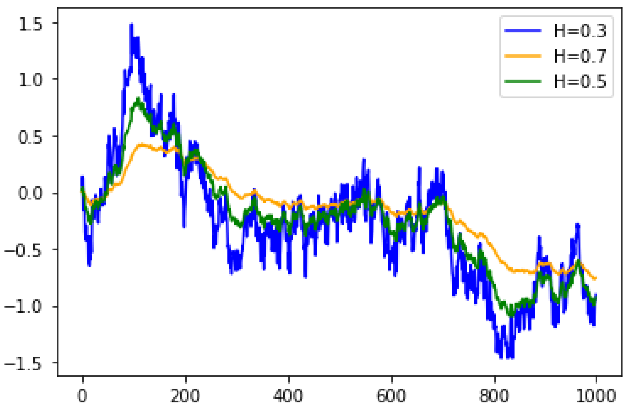
Some simulations of the fBm with $H=0.7,0.5$ and $0.3$ are shown in Figure 1.

3. Malliavin Calculus for Brownian Motion

Malliavin calculus was introduced by Malliavin [40] and has become an important tool in stochastic analysis because the range of its applied and theoretical applications has been increased enormously. In particular, using Malliavin calculus, we can determine if a random variable has a smooth density, which was its original motivation, providing an explicit expression of Clark’s formula, which is now known as the Clark–Haussmann–Ocone formula (see (9)), and dealing with problems related to quantitative finance (see Alòs and García-Lorite [37], Malliavin and Thalmaier [41], and Di Nunno et al. [42], amongst others).

Malliavin calculus is mainly based on three operators: the derivative operator and its adjoint (divergence operator), and the number operator. In Wiener space, Gaveau and Trauber [43] proved that the divergence operator agrees with the Skorohod integral [44], which is an extension of Itô’s integral, which allows us to integrate processes that are not necessarily adapted to the filtration generated by the Brownian motion W. So, Malliavin calculus also becomes an important tool for considering problems where Itô’s calculus is not able to be applied since the integrands are not necessarily adapted to the underlying filtration, as shown by the analysis in León et al. [45] of a financial market with an insider. Hence, we might think that Malliavin calculus only serves to analyze phenomena that are modeled by anticipating systems or stochastic differential equations with anticipating integrals that integrate non-adapted processes; however, Malliavin calculus is useful in several applied problems in several areas, in particular, in finance. The Clark–Haussman–Ocone representation in Formula (9), the integration by parts (6), and anticipating Itô’s Formula (10) have proved useful in financial applications as the computation of hedging strategies, the efficient computation of the Greeks (the sensitivity of derivative prices with respect to the market parameters), and the analysis of the at-the-money implied volatility (see [37] and the references therein).

Now, we introduce the derivative operator (in the Malliavin calculus sense) and the divergence operator in order to establish the notation that we use in the remainder of this paper. Let $\mathcal{S}$ be the set of all smooth random variables of the form

$$F=f(W_{t_1},\dots ,W_{t_n}),$$

(5)

with $t_1,\dots ,t_n\in [0,T]$ and $f\in C_b^{\infty }\left({\mathbb{R}}^n\right)$ (i.e., f and all its partial derivatives are bounded). The derivative of the smooth functional F described by (5) is defined as the stochastic process, in $L^2(\mathsf{\Omega }\times [0,T])$,

$$D_{s}F=\sum _{j=1}^n\frac{\partial f}{\partial x_j}(W_{t_1},\dots ,W_{t_n})1_{[0,t_j]}\left(s\right),s\in [0,T].$$

In general, the iterated derivative operator of a random variable F (as in (5)) is defined by

$$D_{s_1,\dots ,s_m}^{m}F=D_{s_1}\dots D_{s_m}F,s_1,\dots ,s_m\in [0,T].$$

Nualart [46] stated that these operators are closable from $L^p\left(\mathsf{\Omega }\right)$ into $L^p(\mathsf{\Omega };L^2[0,T])$ for any $p\ge 1$, and we denote by ${\mathbb{D}}^{n,p}$ the closure of $\mathcal{S}$ with respect to the norm

$${\left|\right|F\left|\right|}_{n,p}={\left(E{\left|F\right|}^p+\sum _{i=1}^{n}E\left|\right|D^{i}F{\left|\right|}_{L^2\left({[0,T]}^i\right)}^p\right)}^{\frac{1}{p}}.$$

Sometimes D and ${\mathbb{D}}^{n,p}$ are denoted by $D^W$ and ${\mathbb{D}}^{n,p,W}$, respectively, if we are dealing with another Brownian motions.

The adjoint of the derivative operator $D:{\mathbb{D}}^{1,2}\subset L^2\left(\mathsf{\Omega }\right)\to L^2(\mathsf{\Omega }\times [0,T])$ is the divergence operator $\delta$, also called the Skorohod integral in this case. That is, the domain of $\delta$, denoted by Dom $\delta$, is the set of processes $u\in L^2(\mathsf{\Omega }\times [0,T])$ such that there exists $\delta \left(u\right)\in L^2\left(\mathsf{\Omega }\right)$ satisfying the duality relation

$$E\left(\delta \left(u\right)F\right)=E\left({\int }_0^T\left(D_{s}F\right)u_{s}ds\right),\mathrm{for}\mathrm{every}F\in \mathcal{S}.$$

(6)

Sometimes, we use the notation $\delta \left(u\right)={\int }_0^T{u}_{s}d{W}_s$. Let $L_{a,T}^2$ be the family of all the square and adapted process to the filtration ${\mathcal{F}}^W$ generated by W. It is known that $\delta$ is an anticipating integral in the sense that $L_{a,T}^2$ is included in Dom $\delta$ and $\delta$ agrees with the Itô integral on $L_{a,T}^2$. We also know that the space ${\mathbb{L}}^{1,2}=L^2(0,T;{\mathbb{D}}^{1,2})$ is included in the domain of $\delta$. For details, the reader can consult Nualart [46].

The Malliavin calculus has been extended to isonormal Gaussian processes (see, for example, Nualart [46] for details). For completeness of the description, we briefly explain how this extension of Malliavin calculus includes d-dimensional Brownian motions.

Let $\mathcal{H}$ be a real separable Hilbert space and $(\mathsf{\Omega },\mathcal{F},P)$ be a complete probability space.

Definition 1.

A family $W=\left\{W\right(h):h\in \mathcal{H}\}$ defined on $(\mathsf{\Omega },\mathcal{F},P)$ is called an isonormal Gaussian process if it is a Gaussian stochastic process indexed by $\mathcal{H}$ such that

$$E\left(W\left(h\right)\right)=0andE\left(W\left(h\right)W\left(g\right)\right)={\langle h,g\rangle }_{\mathcal{H}},forh,g\in \mathcal{H}.$$

Now a random variable F belongs to the family of smooth functional $\mathcal{S}$ if it has the form

$$F=f(W\left(h_1\right),\dots ,W\left(h_n\right)),$$

(7)

with $h_i\in \mathcal{H}$, f is as in (5), and $DF$ is the $\mathcal{H}$-valued random variable

$$DF=\sum _{j=1}^n\frac{\partial f}{\partial x_j}(W\left(h_1\right),\dots ,W\left(h_n\right))h_j.$$

For $m\in \mathbb{N}$ and F given by (7), the derivative $D^{m}F$ is now an ${\mathcal{H}}^{\otimes m}$. For instance

$$D^{2}F=\sum _{i,j=1}^n\frac{{\partial }^{2}f}{\partial x_j{x}_i}(W\left(h_1\right),\dots ,W\left(h_n\right))h_j\otimes h_i.$$

As before, the domain ${\mathbb{D}}^{m,p}\subset L^p\left(\mathsf{\Omega }\right)$ of the close extension of $D^m$ is the closure of $\mathcal{S}$ with respect to the norm

$${\left|\right|F\left|\right|}_{m,p}={\left(E{\left|F\right|}^p+\sum _{i=1}^{m}E\left|\right|D^{i}F{\left|\right|}_{{\mathcal{H}}^{\otimes m}}^p\right)}^{\frac{1}{p}}.$$

Instead of (6), the divergence operator $\delta :Dom\delta \subset L^2(\mathsf{\Omega };\mathcal{H})\to L^2\left(\mathsf{\Omega }\right)$ is characterized by the duality relation

$$E\left(\delta \left(u\right)F\right)=E\left({\langle DF,u\rangle }_{\mathcal{H}}\right),\mathrm{for}\mathrm{every}F\in \mathcal{S}.$$

(8)

It means that $u\in L^2(\mathsf{\Omega };\mathcal{H})$ is in the domain of the divergence operator if and only if there exists a square integrable random variable $\delta \left(u\right)$, such that (8) holds.

Example 1.

Let $B=(B^1,\dots ,B^d)=\left\{B_t:t\in [0,T]\right\}$ be a d-dimensional Brownian motion. In this case, for $\mathcal{H}=L^2\left([0,T];{\mathbb{R}}^d\right)$, we define

$$\begin{array}{c}\hfill W\left(h\right)=\sum _{i=1}^d{\int }_0^T{h}^i\left(s\right)d{B}_s^{i}h\in \mathcal{H}.\end{array}$$

Then, it is easy to show that $W=\left\{W\left(h\right):h\in \mathcal{H}\right\}$ is an isonormal Gaussian process on $\mathcal{H}$.

The integral representation for functionals of the Wiener process has been an important tool in hedging contingent claims in mathematical finance. Namely, let B be the d-dimensional Brownian motion in Example 1 and $F\in L^2(\mathsf{\Omega },{\mathcal{F}}_T^B,P)$, where ${\left({\mathcal{F}}_t^B\right)}_{t\in [0,T]}$ is the filtration generated by B. Then, there exists a unique ${\mathcal{F}}_t^B$-adapted process $\psi$ in $L^2(\mathsf{\Omega }\times [0,T];{\mathbb{R}}^d)$ such that

$$F=E\left(F\right)+{\int }_0^T{\psi }_{t}d{B}_t=E\left(F\right)+\sum _{i=1}^d{\int }_0^T{\psi }_t^{i}d{B}_t^i.$$

However, in general, it is not easy to determine the ${\mathbb{R}}^d$-valued process $\psi$. This process was first calculated in the case where F has a derivative in the Fréchet sense by Clark [47]. Later, this problem was considered by Haussmann [48] when F is a functional of a solution of a stochastic differential equation driven by B. In the mid-1980s, Ocone [49] wrote $\psi$ in terms of the derivative $DF$. For $F\in {\mathbb{D}}^{1,2}$, we have

$$F=E\left(F\right)+{\int }_0^{T}E\left[D_{t}F|{\mathcal{F}}_t^B\right]d{B}_t=E\left(F\right)+\sum _{i=1}^d{\int }_0^{T}E\left[D_t^{B^i}F|{\mathcal{F}}_t^B\right]d{B}_t^i.$$

(9)

This formula was extended to random variables in ${\mathbb{D}}^{1,1}$ by Karatzas et al. [50], and applied by Ocone and Karatzas [51] to find hedging strategies in complete financial markets driven by B. The proof of (9) is based in the chaos decomposition of random variables using multiple Itô–Wiener integrals. In order to provide an idea of the proof and to simplify the notation, assume that $d=1$. So, the chaos decomposition result implies that

$$F=\sum _{n=0}^{\infty }{I}_n\left(f_n\right),\mathrm{in}{L}^2\left(\mathsf{\Omega }\right).$$

Here, $f_n\in L^2\left({[0,T]}^n\right)$ is a symmetric function, $I_0\left(f_0\right)=E\left(F\right)$ and $I_n\left(f_n\right)$ is the iterated integral

$$I_n\left(f_n\right)=n!{\int }_0^T{\int }_0^{t_n}\cdots {\int }_0^{t_2}{f}_n(t_1,\dots ,t_n)d{B}_{t_1}\cdots d{B}_{t_n}.$$

Then, (9) follows by observing that $D_t{I}_n\left(f_n\right)=n{I}_{n-1}\left(f_n(·,t)\right)$, $t\in [0,T]$, where $\delta$ is an extension of the Itô integral and

$$n\delta \left(I_{n-1}\left(f(t_1,\dots ,t_{n-1},t)1_{\{t_1\vee \dots \vee t_{n-1}\le t\}}\right)\right)=I_n\left(f_n\right),n\ge 1.$$

The reader can consult Nualart [46] for details.

From Example 1, we can consider the divergence operator with respect to a d-dimensional Brownian motion and apply Itô-type formulas for this operator. For instance, we can follow the ideas of Nualart and Pardoux [52] to deal with processes of the form $t\mapsto F(t,X_t,Y_t)$ with $F\in C^{1,2,2}([0,T]\times {\mathbb{R}}^2)$ such that F and its partial derivatives evaluated at $(t,X_t,Y_t)$ are bounded by a constant, $Y_{·}={\int }_{·}^T{\theta }_{s}ds$ and

$$X_t=x+{\int }_0^t{u}_{s}ds+{\int }_0^t{v}_s\left(\rho d{W}_s+\sqrt{1-\rho }d{B}_s\right),t\in [0,T].$$

Here, $x\in \mathbb{R}$, W, and B are two independent Brownian motions; u, v, and $\theta$ are three square-integrable and adapted processes to the filtration generated by W with $\theta \in L^2([0,T];{\mathbb{D}}^{1,2,W})$, and $\rho \in (-1,1)$. In this case, we have

$$\begin{array}{ccc}\hfill F(t,X_t,Y_t)& =& F(0,x,Y_0)+{\int }_0^t{\partial }_{s}F(s,X_s,Y_s)ds+{\int }_0^t{\partial }_{x}F(s,X_s,Y_s)u_{s}ds\hfill \\ & & +{\int }_0^t{\partial }_{x}F(s,X_s,Y_s)\left(\rho d{W}_s+\sqrt{1-\rho }d{B}_s\right)\hfill \\ & & -{\int }_0^t{\partial }_{y}F(s,X_s,Y_s){\theta }_{s}ds+\frac{1}{2}{\int }_0^t{\partial }_{xx}^{2}F(s,X_s,Y_s)v_s^{2}ds\hfill \\ & & +\rho {\int }_0^t{\partial }_{xy}^{2}F(s,X_s,Y_s)\left({\int }_s^T{D}_s^W{\theta }_{r}dr\right)v_{s}ds,t\in [0,T].\hfill \end{array}$$

(10)

Note that the stochastic integral with respect to W is in the Skorohod sense and that we need to use Malliavin calculus in order to state the last Itô formula because process Y is not adapted to the filtration generated by W and B. We also obtain the classical Itô formula when $\theta$ is a deterministic function since, in this case, ${\int }_{·}^T{D}_s^W{\theta }_{r}dr\equiv 0$, which follows easily from the definition of the Malliavin derivative. Notably, Malliavin calculus allows us to consider Itô’s formulas with coefficients not necessarily adapted to the underlying filtration, which satisfy suitable hypotheses depending on the derivative operator D (see, for instance, Nualart and Pardoux [52] and Nualart [46,53]). The proof of (10) uses Taylor’s theorem as that of the classical Itô’s formula. Hence, given a partition $\pi =\{0=t_0<t_1<\dots ,t_n=T\}$, we consider the term

$${\partial }_{x}F(t_{i-1},X_{t_{i-1}},Y_{t_{i-1}}){\int }_{t_{i-1}}^{t_i}{v}_s\left(\rho d{W}_s+\sqrt{1-\rho }d{B}_s\right).$$

Thus, considering Y as independent of B, we obtain

$$\begin{array}{c}\hfill {\displaystyle \sqrt{1-\rho }{\partial }_{x}F(t_{i-1},X_{t_{i-1}},Y_{t_{i-1}}){\int }_{t_{i-1}}^{t_i}{v}_{s}d{B}_s}\\ \hspace{1em}\hspace{1em}=\sqrt{1-\rho }{\int }_{t_{i-1}}^{t_i}{v}_s{\partial }_{x}F(t_{i-1},X_{t_{i-1}},Y_{t_{i-1}})d{B}_s,\hfill \end{array}$$

as in the proof of the classical Itô formula. However,

$$\begin{array}{c}{\displaystyle \rho {\partial }_{x}F(t_{i-1},X_{t_{i-1}},Y_{t_{i-1}}){\int }_{t_{i-1}}^{t_i}{v}_{s}d{W}_s}\hfill \\ \hspace{1em}\hspace{1em}=\rho {\int }_{t_{i-1}}^{t_i}{v}_s{\partial }_{x}F(t_{i-1},X_{t_{i-1}},Y_{t_{i-1}})d{W}_s\hfill \\ \hspace{1em}\hspace{1em}\hspace{1em}+\rho {\int }_{t_{i-1}}^{t_i}{v}_s{D}_s^W\left({\partial }_{x}F(t_{i-1},X_{t_{i-1}},Y_{t_{i-1}})\right)ds\hfill \\ \hspace{1em}\hspace{1em}=\rho {\int }_{t_{i-1}}^{t_i}{v}_s{\partial }_{x}F(t_{i-1},X_{t_{i-1}},Y_{t_{i-1}})d{W}_s\hfill \\ \hspace{1em}\hspace{1em}\hspace{1em}+\rho {\int }_{t_{i-1}}^{t_i}{v}_s{\partial }_{xy}^{2}F(t_{i-1},X_{t_{i-1}},Y_{t_{i-1}})D_s^W{Y}_{t_{i-1}}ds\hfill \end{array}$$

because Y is not an process adapted to the filtration generated by W and the property

$$F{\delta }^W\left(u\right)={\delta }^W\left(Fu\right)+{\int }_0^T{u}_s{D}_s^{W}Fds,$$

which is true under suitable conditions (see Nualart [46] for details). Consequently, the last integral in the right-hand of (10) is related to the integral $\rho {\int }_{t_{i-1}}^{t_i}{v}_s{\partial }_{xy}^{2}F(t_{i-1},X_{t_{i-1}},Y_{t_{i-1}})D_s^W{Y}_{t_{i-1}}ds$, which is zero if $\theta$ is deterministic.

4. Stochastic Volatility Models and the Implied Volatility

4.1. The Black-Scholes Model and the Concept of Implied Volatility

The most well-known risk-neutral model for asset prices S is the Black-Scholes model [1]:

$$d{S}_t=r{S}_{t}dt+\sigma S_{t}d{B}_t,t\in [0,T],$$

(11)

where $T>0$, r denotes the interest rate, $\sigma$ is the volatility parameter, and B represents a standard Brownian motion defined in a probability space $(\mathsf{\Omega },\mathcal{F},P)$. Notice that this model assumes that S is a geometric Brownian motion, and then

$$S_t=S_{0}exp\left(\left(r-\frac{{\sigma }^2}{2}\right)t+\sigma B_t\right),t\in [0,T],$$

due to Itô’s formula. For the sake of simplicity, it is common to work with the log-price defined as $X=ln\left(S\right)$. Notice that X is a Gaussian process, and it satisfies

$$d{X}_t=\left(r-\frac{1}{2}{\sigma }^2\right)dt+\sigma d{B}_t,t\in (0,T].$$

Under this model, the value V of a European call option with payoff ${(S_T-K)}_{+}$, where K is the strike price, is given at every $t\in [0,T]$ by

$$V_t=e^{-r(T-t)}{E}_t\left[{(S_T-K)}_{+}\right]=BS(t,X_t,K,\sigma ),$$

where $E_t$ denotes the conditional expectation with respect to the $\sigma$-algebra generated by B and $BS$ represents the price of an European call option under the classical Black-Scholes model with constant volatility $\sigma$, current log stock price x, time to maturity $T-t,$ strike price K, and interest rate $r.$ That is,

$$BS(t,x,K,\sigma )=e^{x}N\left(d_{+}\right)-K{e}^{-r(T-t)}N\left(d_{-}\right),$$

where N denotes the cumulative probability function of the standard normal law and

$$d_{\pm }:=\frac{x-x_t^{*}}{\sigma \sqrt{T-t}}\pm \frac{\sigma }{2}\sqrt{T-t},$$

with $x_t^{*}:=lnK-r(T-t).$

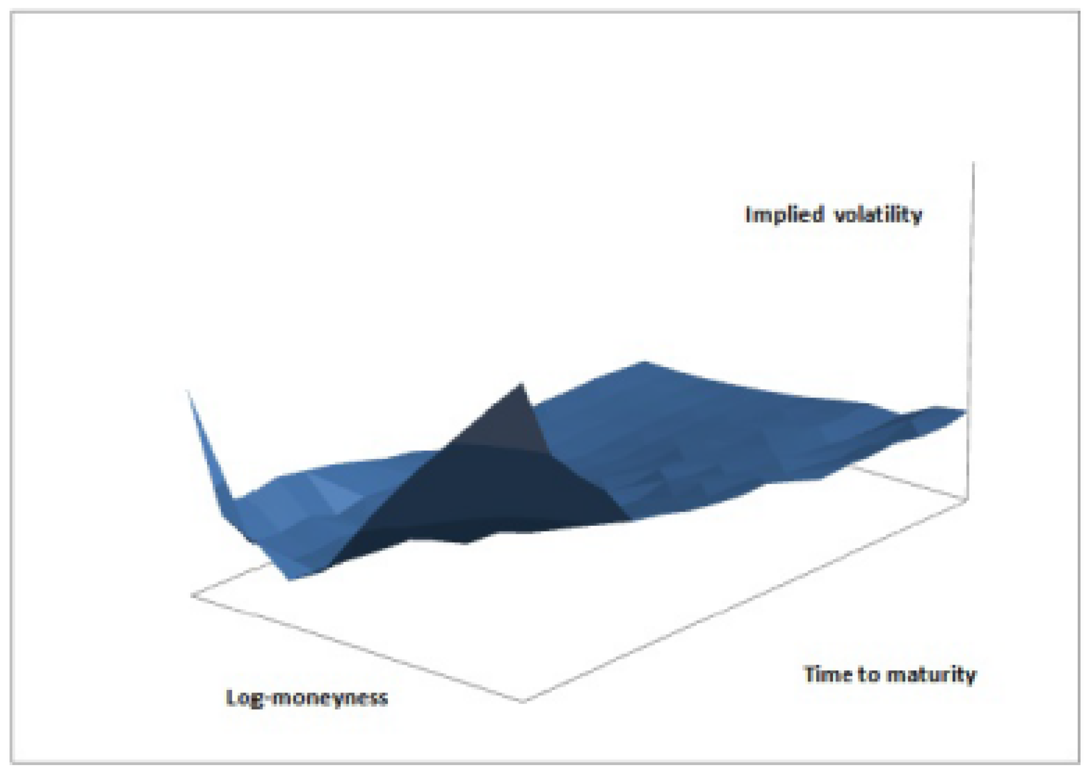
Given an observed market price V of some European call, we define the implied volatility I as the volatility that fits this empirical price. That is, the implied volatility is defined by $V_t=BS(t,X_t,K,I)$ (notice that I is well-defined as $BS$ is invertible). Under the Black-Scholes model (11), these implied volatilities should be constant, not depending on the parameters K and T. However, empirical implied volatilities are not constant. The representation of the observed market implied volatility as a function of the strike (or, more often, as a function of the log-moneyness) and time to maturity is called the implied volatility surface. As the implied volatility surface is not flat and the implied volatility depends on the moneyness and time to maturity, the Black-Scholes model (11) is not able to reflect the complexity of option prices in the market. Because of this, several extensions of this model have been proposed in the literature. One of the most common is to allow the volatility to be a stochastic process, adapted to some other Brownian motion W that can be correlated with B, as we see in the following section. Recently, Fink [54] considered the Black-Scholes setting to deal with models driven by Molchan–Golosov fractional Lévy processes. These models are free of arbitrage. Consequently, a version of the fundamental theorem of asset pricing is stated. Therefore, it is possible to determine explicit formulas for European call options.

4.2. Stochastic Volatility Models

One of the most common extensions of the Black-Scholes model (11) is to assume that the volatility is also a random process, that is, asset prices follow a process of the form

$$d{S}_t=r{S}_{t}dt+{\sigma }_t{S}_t(\rho d{W}_t+\sqrt{1-{\rho }^2}d{B}_t),t\in [0,T],$$

(12)

for some other Brownian motion W independent of B and for some correlation parameter $\rho \in (-1,1)$, and $\sigma$ is a process adapted to the filtration generated by W. When $\sigma$ is a diffusion process, models of the form (12) are called stochastic volatility models. Classical popular examples both in theory and practice include:

• The Heston model, where the volatility satisfies

  $$d{\sigma }_t^2=k({\sigma }_t^2-\theta )dt+\nu \sqrt{{\sigma }_t^2}d{W}_t,$$

  (13)

  for some positive constants $k,\theta$, and $\nu$;
• The SABR model, with

  $$d{\sigma }_t=\nu {\sigma }_{t}d{W}_t,$$

  (14)

  for some positive $\nu$.

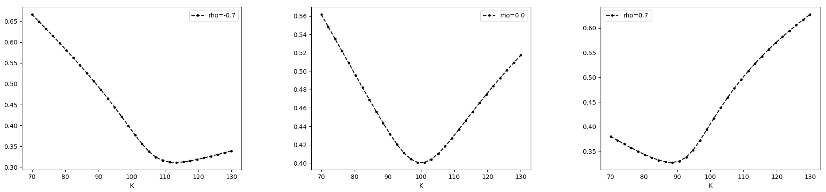
Stochastic volatility models are able to describe some properties of empirical option prices as skews and smiles (see, for example, Lee [55]). With fixed T, we denote by skew the plot of the implied volatility as a function of the strike (or, alternatively, as a function of the log-moneyness $X_t-x_t^{*}$) (Figure 2). If this skew is locally convex with a minimum in the at-the-money strike (U-plotted), we call it a smile (Figure 2). Smiles appear in models with $\rho =0$, whereas in the correlated case $\rho \ne 0$, this skew has a slope that can be positive or negative depending on the sign of the correlation parameter.

Moreover, skews and smiles are more pronounced for short maturities and they flatten as T increases (Figure 3).

Even when stochastic volatility models can describe skews and smiles for a fixed maturity, they are not able to reproduce the empirical term structure of implied volatilities; that is, they cannot replicate all these smiles at the same time and they cannot reproduce the whole implied volatility surface. In general, the empirical skew and smile effects are more pronounced for short and intermediate maturities than those predicted by stochastic volatility models (see Lee [55]). For example, Figure 4 shows the classical short-end of the implied volatility skew. The empirical skew slope used to be of order $O(T^{-\frac{1}{2}})$ (see again [55]), a phenomenon that is not explained by classical volatility models, where the volatility is assumed to be a diffusion process.

There have been many attempts to overcome this issue. For example, adding jumps in (12) allows the creation of skews in the implied volatility that are stronger for short maturities (see, for example, Cont and Tankov [56]). Another approach proposes diffusions with parameters that depend on the maturity date (see Fouque et al. [57]). In this paper, we focus on the fractional volatility models, where the driven process is not a Brownian motion, but a fBm, as given in Section 2. We introduce the intuition behind these models in the following section. This intuition is based on the properties of the volatility process that are linked to the empirical implied volatility surface. Even when we focus on the origin of the use of the fBm in volatility modeling, we notice that it has recently found interesting applications in other financial problems, such as in the joint calibration of the S&P and the VIX indexes. In particular, fractional volatilities can reproduce a positive VIX skew (see, for example, [58,59]), being a study of other volatility indexes (such as the VSTOOXX and OVX), which is an interesting research line.

5. Intuition behind Fractional Volatility Models

5.1. An Expansion for the Implied Volatility

In order to propose a model, we have to deeply understand the behavior of the implied volatility. We stated that in the Black-Scholes case (11), the volatility is constant. What happens exactly if the volatility is not constant?

5.1.1. The Deterministic Case

Let us assume first the case where the volatility $\sigma =\{{\sigma }_t,t\in [0,T]\}$ is a deterministic function of time. Then, a direct application of Itô’s formula gives us, for every $t\in [0,T]$, that

$$S_T=S_{t}exp\left({\int }_t^T\left(r-\frac{1}{2}{\sigma }_s^2\right)ds+{\int }_t^T{\sigma }_{s}d{B}_s\right),$$

which implies that, conditioned to ${\mathcal{F}}_t^B$, $X_T:=ln\left(S_T\right)$ is Gaussian, with mean $X_t+{\int }_t^T\left(r-\frac{1}{2}{\sigma }_s^2\right)ds$ and variance ${\int }_t^T{\sigma }_s^{2}ds$. That is, fixed t asset prices have the same distribution as in a Black-Scholes model (11) with volatility $\sqrt{\frac{1}{T-t}{\int }_t^T{\sigma }_s^{2}ds}$. Then, the price $V_t$ of a European call with maturity T and strike K is given by

$$V_t=BS\left(t,X_t,K,\sqrt{\frac{1}{T-t}{\int }_t^T{\sigma }_s^{2}ds}\right).$$

Thus, it follows that the implied volatility $I_t$ does not depend on the strike, and is equal to

$$I_t=\sqrt{\frac{1}{T-t}{\int }_t^T{\sigma }_s^{2}ds}.$$

5.1.2. The Stochastic Volatility Case with $\rho =0$

Now, what happens if the volatility is random? Let us assume for the sake of simplicity that $\rho =0$. Then, conditioned to the $\sigma$-algebra generated by W, we are in the same scenario as in the deterministic case, that is,

$$V_t=E_t\left(BS\left(t,X_t,K,\sqrt{\frac{1}{T-t}{\int }_t^T{\sigma }_s^{2}ds}\right)\right),$$

(15)

where $E_t(·)=E(·|{\mathcal{F}}_t^W\vee {\mathcal{F}}_t^B)$. The above formula is known as the Hull and White formula (see, for example, Fouque et al. [57]). Notice that, again, the behavior of the implied volatility depends on the behavior of $\sqrt{\frac{1}{T-t}{\int }_t^T{\sigma }_s^{2}ds}$. Let us now denote

$$v_t=\sqrt{\frac{1}{T-t}{\int }_t^T{\sigma }_s^{2}ds}$$

and

$${\widehat{v}}_t=\sqrt{\frac{1}{T-t}{\int }_t^T{E}_t\left({\sigma }_s^2\right)ds}.$$

A direct Taylor approach and the delta–vega–gamma relationship

$$\frac{\partial BS}{\partial \sigma }(t,x,K,\sigma )\frac{1}{\sigma (T-t)}=\left(\frac{\partial }{\partial x^2}-\frac{\partial }{\partial x}\right)BS(t,x,K,\sigma )$$

show us that the expression in the Hull and White formula can be expanded as

$$\begin{array}{ccc}& & E_t\left(BS\left(t,X_t,K,v_t\right)\right)\hfill \\ & & =BS\left(t,X_t,K,{\widehat{v}}_t\right)\hfill \\ & & +\frac{1}{2}{E}_t\left[\left(\frac{\partial }{\partial x^2}-\frac{\partial }{\partial x}\right)BS\left(t,X_t,K,{\widehat{v}}_t\right)\left({\int }_t^T{\sigma }_s^{2}ds-{\int }_t^T{E}_t\left({\sigma }_s^2\right)ds\right)\right.\hfill \\ & & +\frac{1}{8}\left.{\left(\frac{\partial }{\partial x^2}-\frac{\partial }{\partial x}\right)}^{2}BS\left(t,X_t,K,{\widehat{v}}_t\right){\left({\int }_t^T{\sigma }_s^{2}ds-{\int }_t^T{E}_t\left({\sigma }_s^2\right)ds\right)}^2+\dots \right]\hfill \end{array}$$

Notice that the second term in the right-hand-side in the above equation is zero. Then, we can write

$$\begin{array}{ccc}& & E_t\left(BS\left(t,X_t,K,v_t\right)\right)\hfill \\ & & =BS\left(t,X_t,K,{\widehat{v}}_t\right)\hfill \\ & & +\left[\frac{1}{8}{\left(\frac{\partial }{\partial x^2}-\frac{\partial }{\partial x}\right)}^{2}BS\left(t,X_t,K,{\widehat{v}}_t\right)E_t\left({\left({\int }_t^T{\sigma }_s^{2}ds-{\int }_t^T{E}_t\left({\sigma }_s^2\right)ds\right)}^2\right)+\cdots \right]\hfill \\ & & =:\left(BS\left(t,X_t,K,{\widehat{v}}_t\right)\right)+A_t+\cdots .\hfill \end{array}$$

(16)

Now, we can obtain a Taylor expansion for the implied volatility:

$$\begin{array}{ccc}\hfill & & I_t=B{S}^{-1}(\left(BS\left(t,X_t,K,{\widehat{v}}_t\right)+A_t+\cdots \right)\hfill \\ & & ={\widehat{v}}_t+\frac{1}{\frac{\partial BS}{\partial \sigma }(t,x,K,{\widehat{v}}_t)}{A}_t+\cdots .\hfill \end{array}$$

(17)

Then, as

$$\frac{\partial BS}{\partial \sigma }=\frac{e^x}{\sqrt{2\pi }}exp\left(-\frac{d_{+}^2\left(\sigma \right)}{2}\right)\sqrt{T-t}$$

and

$$\begin{array}{ccc}& & {\left(\frac{\partial }{\partial x^2}-\frac{\partial }{\partial x}\right)}^{2}BS\left(t,X_t,K,{\widehat{v}}_t\right)\hfill \\ & & =\frac{e^x}{\sqrt{2\pi (T-t)}}exp\left(-\frac{d_{+}^2\left({\widehat{v}}_t\right)}{2}\right)\frac{d_{+}^2\left({\widehat{v}}_t\right)-{\widehat{v}}_t{d}_{+}\left({\widehat{v}}_t\right)\sqrt{T-t}-1}{{\widehat{v}}_t^3(T-t)},\hfill \end{array}$$

(18)

Equality (17) reads as

$$\begin{array}{ccc}\hfill I_t& =& {\widehat{v}}_t+\frac{d_{+}^2\left({\widehat{v}}_t\right)-{\widehat{v}}_t{d}_{+}\left({\widehat{v}}_t\right)\sqrt{T-t}-1}{{\widehat{v}}_t^3{(T-t)}^2}{E}_t{\left({\int }_t^T{\sigma }_s^{2}ds-{\int }_t^T{E}_t\left({\widehat{v}}_t^2\right)ds\right)}^2\hfill \\ & & +\cdots .\hfill \end{array}$$

(19)

Notice that this expansion writes the implied volatility as the sum of the term ${\widehat{v}}_t$, which does not depend on the strike, and a second term that is quadratic on the log-moneyness and it appears multiplied by the variance of the integrated variance ${\int }_t^T{\sigma }_s^{2}ds$. Then, smiles and skews are more pronounced when the variability of this integrated volatility is higher, that is, for high-variance volatilities.

5.1.3. The Stochastic Volatility Case with $\rho \ne 0$

Let us consider now the correlated $\rho \ne 0$. Again, taking conditional expectations with respect to the $\sigma$-algebra generated by W, we obtain

$$V_t=E_t\left(BS\left(t,X_t{\psi }_t,K,\sqrt{(1-{\rho }^2)\frac{1}{T-t}{\int }_t^T{\sigma }_s^{2}ds}\right)\right),$$

where ${\psi }_t=\rho {\int }_t^T{\sigma }_{s}d{W}_s$ (see Romano and Touzi [60] and Willard [61]). Then, a similar Taylor expansion as in the uncorrelated case shows us that the skews in this case are directly connected to the variability in the integrated variance ${\int }_t^T{\sigma }_s^{2}ds$, as well as to the covariance between this integrated variance and the random variable ${\psi }_t$. More precisely, the delta–vega–gamma relationship allows us to write

$$\frac{{\partial }^{2}BS}{\partial \sigma \partial x}(t,x,K,\sigma )\frac{1}{\sigma (T-t)}=\frac{\partial }{\partial x}\left(\frac{\partial }{\partial x^2}-\frac{\partial }{\partial x}\right)BS(t,x,K,\sigma )$$

and then, after taking expectations, the second-order Taylor expansion reads as

$$\begin{array}{ccc}& & V_t=BS\left(t,X_t,K,{\widehat{v}}_t\right)\hfill \\ & & +\frac{1}{2}\left[\frac{\partial }{\partial x}\left(\frac{\partial }{\partial x^2}-\frac{\partial }{\partial x}\right)BS\left(t,X_t,K,{\widehat{v}}_t\right)\right.\hfill \\ & & \times E_t\left(\left({\int }_t^T{\sigma }_s^{2}ds-{\int }_t^T{E}_t\left({\sigma }_s^2\right)ds\right){\psi }_t\right)\hfill \\ & & +\frac{1}{8}{\left(\frac{\partial }{\partial x^2}-\frac{\partial }{\partial x}\right)}^{2}BS\left(t,X_t,K,{\widehat{v}}_t\right)\hfill \\ & & \times \left.(1-{\rho }^2)E_t{\left({\int }_t^T{\sigma }_s^{2}ds-{\int }_t^T{E}_t\left({\sigma }_s^2\right)ds\right)}^2+\dots \right].\hfill \end{array}$$

(20)

Now, since

$$\begin{array}{ccc}& & \frac{\partial }{\partial x}\left(\frac{\partial }{\partial x^2}-\frac{\partial }{\partial x}\right)BS\left(t,x,K,\sigma \right)\hfill \\ & =& \frac{e^x}{\sigma \sqrt{2\pi (T-t)}}exp\left(-\frac{d_{+}^2\left(\sigma \right)}{2}\right)\left(1-\frac{d_{+}\left(\sigma \right)}{\sigma \sqrt{T-t}}\right),\hfill \end{array}$$

(21)

similar arguments as before allow us to write

$$\begin{array}{ccc}\hfill I_t& =& {\widehat{v}}_t\hfill \\ & +& \frac{1}{(T-t)}\left(1-\frac{d_{+}\left({\widehat{v}}_t\right)}{{\widehat{v}}_t\sqrt{T-t}}\right)E_t\left(\left({\int }_t^T{\sigma }_s^{2}ds-{\int }_t^T{E}_t\left({\sigma }_s^2\right)ds\right){\psi }_t\right)\hfill \\ & +& \frac{d_{+}^2\left({\widehat{v}}_t\right)-\sigma d_{+}\left({\widehat{v}}_t\right)\sqrt{T-t}-1}{{\widehat{v}}_t^3{(T-t)}^2}(1-{\rho }^2)E_t{\left({\int }_t^T{\sigma }_s^{2}ds-{\int }_t^T{E}_t\left({\sigma }_s^2\right)ds\right)}^2\hfill \\ & +& \cdots \hfill \end{array}$$

(22)

From the above, we deduce that the covariance between ${\int }_t^T{\sigma }_s^{2}ds$ and $\psi$ introduces a linear term in the correlation expansion.

5.2. The Clark Ocone Formula for the Integrated Variance

Now the question is how to construct a volatility model so that the variance of ${\int }_t^T{\sigma }_s^{2}ds$ is higher for long and short maturities, where classical diffusion models fail in reproducing the implied volatility surface. Let us study the variability in this random variable. Due to the Clark–Ocone–Haussman Formula (9)

$${\sigma }_s^2=E_t\left({\sigma }_s^2\right)+{\int }_t^s{E}_r\left(D_r^W{\sigma }_s^2\right)d{W}_r,$$

for $t<s$. Fubini’s theorem for the Itô integral leads to

$$\begin{array}{ccc}\hfill {\int }_t^T{\sigma }_s^{2}ds& =& {\int }_t^T{E}_t\left({\sigma }_s^2\right)ds+{\int }_t^T\left({\int }_t^s{E}_r\left(D_r^W{\sigma }_s^2\right)d{W}_r\right)ds\hfill \\ & & ={\int }_t^T{E}_t\left({\sigma }_s^2\right)ds+{\int }_t^T\left({\int }_r^T{E}_r\left(D_r^W{\sigma }_s^2\right)ds\right)d{W}_r.\hfill \end{array}$$

(23)

Thus, the variability in the integrated variance is provided by the term

$${\int }_t^T{E}_t{\left({\int }_r^T{E}_r\left(D_r^W{\sigma }_s^2\right)ds\right)}^{2}dr$$

Consider now the case where ${\sigma }_t^2=f\left(W_t^H\right)$,for some deterministic function f and some RLfBm $W^H$ adapted to the filtration generated by W. Then, $D_r^W{\sigma }_s^2=f^{\prime }\left(W_s^H\right){(s-r)}^{H-\frac{1}{2}}$. If $f^{\prime }$ is bounded, the above term behaves like ${(T-t)}^{2H+2}$. In the classical Brownian motion case, this quantity behaves like ${(T-t)}^3$. If $T-t<1$, this variability can be increased by taking $H<1/2$. If $T-t>1$, this variability can be increased by taking $H>1/2$.

Following these ideas, the first fractional volatility model in the literature was presented in Comte and Renault [20], where the authors considered a Hurst parameter $H>1/2$ to describe the slow flattening of smiles and skews as time to maturity increases. In Alòs et al. [9], these models, but with $H<1/2$, were introduced to better describe the short-end of the implied volatility surface. We notice that both approaches are not contradictory: the volatility can be composed of terms with $H>1/2$ and terms with $H<1/2$, with the terms with $H>1/2$ ($H<1/2$) being more relevant at long (short) scales.

6. Some Analytical Results

Consider the stochastic volatility model (12). The log-price $X=log\left(S\right)$ has the form

$$X_t=x+rt-\frac{1}{2}{\int }_0^t{\sigma }_s^{2}ds+{\int }_0^t{\sigma }_s(\rho d{W}_s+\sqrt{1-{\rho }^2}d{B}_s),t\in [0,T].$$

(24)

Remember that the volatility process $\sigma$ is an ${\mathcal{F}}_t^W$-adapted process and, from now on, we assume that it is a square-integrable stochastic process with right-continuous paths bounded below by a positive constant. Note that (24) is a general stochastic volatility model that includes the Heston model [7] and that no particular dynamics are assumed for the volatility process $\sigma$. So, we can even consider rough volatilities (i.e., stochastic volatilities driven by an RLfBm, with $H\in (0,1)$).

6.1. An Extension of the Hull and White Formula

An important application of the anticipating Itô Formula (10) is the study of the extensions of the Hull and White Formula (15) when the volatility and the noises driven the prices are correlated (i.e., $\rho \ne 0$). In particular, it can be proved (see Alòs [10]) that

$$V_t=E_t\left(BS(t,X_t,v_t)\right)+\frac{\rho }{2}{E}_t\left({\int }_t^T{e}^{-r(s-t)}{\partial }_{x}G(s,X_s,v_s){\mathsf{\Lambda }}_{s}ds\right),$$

(25)

with $t\in [0,T]$, $G(t,x,\sigma )=({\partial }_{xx}^2-{\partial }_x)BS(t,x,\sigma )$, and ${\mathsf{\Lambda }}_t:=\left({\int }_t^T{D}_t^W{\sigma }_r^{2}dr\right){\sigma }_t$, and where v is defined as in Section 5.1.2. It means that this price depends on the derivative of the volatility in the Malliavin calculus sense if $\rho \ne 0$. Note that the above representation decomposes option prices as the sum of two terms: the Hull and White term, which coincides with the price in the case $\rho =0$, and a second term due to the correlation.

The idea of the proof of (25) is as follows: From one side, $BS(T,X_T,K,v_T)=V_T$, where $v_T$ is defined as in Section 5.1.2, which allows us to write

$$e^{-rt}{V}_t=E_t\left(e^{-rT}BS(T,X_T,K,v_T)\right).$$

Now, the key point is to apply the anticipating Itô formula given by (10) to the process

$$e^{-r·}BS(·,X_{·},K,v_{·}).$$

This allows us to find a representation for the difference

$$V_t-E_t\left(BS(t,X_t,v_t)\right)$$

as the sum of several terms. Thus, due to the Black-Scholes equation

$$\left({\partial }_t+\frac{1}{2}{\sigma }^2{\partial }_{xx}^2+\left(r-\frac{1}{2}{\sigma }^2\right){\partial }_x-r\right)BS(t,x,K,\sigma )=0$$

and the relations among the gamma, vega, and delta, all the terms in this representation cancel, except that related to the Malliavin derivative of the non-adapted process v. This term corresponds to the last term in (25).

The above approach can be extended to the case of models with jumps using the Itô formula for Lévy processes developed by Solé et al. [62]. This allows us to consider models of the form

$$\begin{array}{ccc}\hfill X_t& =& x+(r-\lambda \widehat{k})t-\frac{1}{2}{\int }_0^t{\sigma }_s^{2}ds\hfill \\ & & +{\int }_0^t{\sigma }_s(\rho d{W}_s+\sqrt{1-{\rho }^2}d{B}_s)+Z_t,t\in [0,T].\hfill \end{array}$$

(26)

(see Alòs et al. [9,63]). Here, Z is a pure jump Lévy process. Thus, we have an extension of some classical models such as the Bates [6] and Heston [7] ones. The reader can consult Barndorff-Nielsen and Shephard [11,12], Cont and Tankov [56], and Medvedev and Scaillet [64] to observe the convenience of including jumps in the price asset dynamics.

An extension of the Hull and White formula under the model (26) was developed by Alòs et al. [9] when $\sigma$ is a stochastic process and Z is a compound Poisson process with intensity $\lambda$, Lévy measure $\nu$, independent of W and $B,$ and with $\widehat{k}=\frac{1}{\lambda }{\int }_{\mathbb{R}}(e^y-1)\nu \left(dy\right)<\infty$. In this case, after proving a suitable Itô formula that allows us to deal with X in (26), it can be proved that (25) becomes an extension of th Hull and White formula given by

$$\begin{array}{ccc}\hfill V_t& =& E\left(BS(t,X_t,v_t)\right|{\mathcal{G}}_t)+\frac{\rho }{2}E\left({\int }_t^T{e}^{-r(s-t)}{\partial }_{x}G(s,X_s,v_s){\mathsf{\Lambda }}_{s}ds|{\mathcal{G}}_t\right)\hfill \\ & & +E\left({\int }_t^T{\int }_{\mathbb{R}}{e}^{-r(s-t)}\left\{BS(s,X_s+y,v_s)-BS(s,X_s,v_s)\right\}\nu \left(dy\right)ds|{\mathcal{G}}_t\right)\hfill \\ & & -\lambda \widehat{k}E\left({\int }_t^T{e}^{-r(s-t)}{\partial }_{x}BS(s,X_s,v_s)ds|{\mathcal{G}}_t\right),t\in [0,T],\hfill \end{array}$$

(27)

with $\mathcal{G}={\mathcal{F}}^W\vee {\mathcal{F}}^B\vee {\mathcal{F}}^Z$.

Note that if $\nu \equiv 0$, then (28) is (25). When Z is a pure Lévy process and $\sigma$ is an adapted process to the filtration generated by W and Z, the above formula takes the form

$$\begin{array}{ccc}\hfill V_t& =& E\left(BS(t,X_t,v_t)\right|{\mathcal{G}}_t)+\frac{\rho }{2}E\left({\int }_t^T{e}^{-r(s-t)}{\partial }_{x}G(s,X_s,v_s){\mathsf{\Lambda }}_{s}ds|{\mathcal{G}}_t\right)\hfill \\ & & +E\left({\int }_t^T{\int }_{\mathbb{R}}{e}^{-r(s-t)}\left\{{\Delta }_{y}BS(s,X_s,v_s)\right.\right.\hfill \\ & & \left.\phantom{{\int }_t^T{\int }_{\mathbb{R}}}\left.-(e^y-1){\partial }_{x}BS(s,X_s,v_s)\right\}\nu \left(dy\right)ds|{\mathcal{G}}_t\right)\hfill \\ & & +E\left({\int }_t^T{\int }_{\mathbb{R}}{e}^{-r(s-t)}{D}_{s,y}^{Z,-}{\Delta }_{y}BS(s,X_s,v_s)y\nu \left(dy\right)ds|{\mathcal{G}}_t\right).\hfill \end{array}$$

Here, ${\Delta }_{y}BS(s,X_s,v_s)=BS(s,X_s+y,v_s)-BS(s,X_s,v_s)$ and $D^Z$ is the two-parameter operator defined via the chaos decomposition approach on the canonical Lévy space. Roughly, $D_{·,0}^Z$ agrees with the derivative operator with respect to the continuous part (Brownian part) of the involved Lévy process and $D_{t,x}$, $x\ne 0$ is the quotient operator given by

$$D_{t,x}F\left(\omega \right)=\frac{F\left({\omega }_{t,x}\right)-F\left(\omega \right)}{x},$$

where ${\omega }_{t,x}$ means that we have added a jump of size x at time t. Finally,

$$D^{Z,-}u(t,y)=L^2(P\otimes dt\otimes x\nu \left(dx\right))-\underset{r\uparrow t,x\uparrow y}{lim}{D}_{t,y}^{Z}u(r,x).$$

We observe that $D_{s,y}^{Z,-}{\Delta }_{y}BS(s,X_s,v_s)=0$ for $(s,y)\in [0,T]\times (\mathbb{R}\backslash \{0\left\}\right)$, if the volatility process $\sigma$ is only ${\mathcal{F}}_t^W$-adapted (i.e., it is independent of Z). For details, the reader is referred to Alòs et al. [63], Jafari and Vives [65], and Solé et al. [62]. This decomposition approach can be extended to the study of exotic options (see, for example, Alòs and León [66], Alòs et al. [67], Merino and Vives [68], and Alòs and León [69]).

6.2. The Derivative of the Implied Volatility

Once we have a Hull and White type formula for a suitable stochastic volatility model, we can determine the derivative of the implied volatility (with respect to the log-strike) in terms of the derivative operator in the Malliavin calculus sense and study the at-the-money short-time behavior of skew slopes. Remember that in our analytical study, we do not assume that the volatility is either a diffusion or a Markov process. We can even consider volatilities driven by an RLfBm introduced in (4). In the following, we briefly explain how the Hull and White type formulas can be used to analyze the short-time behavior of the implied volatility.

Roughly, the Hull and White type formulas established in this section have the form

$$V_t=E_t\left(BS(t,X_t,v_t)\right)+E_t\left({\int }_t^{T}F(s,X_s,v_s)ds\right),t\in [0,T].$$

Consequently,

$$\frac{\partial V_t}{\partial X_t}=E_t\left({\partial }_{x}BS(t,X_t,v_t)\right)+E_t\left({\int }_t^T{\partial }_{x}F(s,X_s,v_s)ds\right),t\in [0,T].$$

(28)

Now, let $I_{·}\left(X_{·}\right)$ be the implied volatility, which satisfies $V_t=BS(t,X_t,K,I_t\left(X_t\right))$ by definition. So, (28) leads us to

$$\begin{array}{c}\hfill {\displaystyle \frac{\partial I_t}{\partial X_t}\left(x_t^{*}\right)}\\ & =& {\left.\frac{E_t\left({\partial }_{x}BS(t,x_t^{*},v_t)\right|{\mathcal{F}}_t)-{\partial }_{x}BS(t,x_t^{*},I_t\left(x_t^{*}\right))+E_t\left({\int }_t^T{\partial }_{x}F(s,X_s,v_s)ds\right)}{{\partial }_{\sigma }BS(t,x_t^{*},I_t\left(x_t^{*}\right))}\right|}_{X_t=x_t^{*}}\hfill \\ & =& {\left.\frac{E_t\left({\int }_t^T({\partial }_{x}F(s,X_s,v_s)-\frac{1}{2}F(s,X_s,v_s))ds\right)}{{\partial }_{\sigma }BS(t,x_t^{*},I_t\left(x_t^{*}\right))}\right|}_{X_t=x_t^{*}},\mathrm{w}.\mathrm{p}.1.\hfill \end{array}$$

(29)

Here, the last equality follows from (28) and that

$${\partial }_x(BS(t,x,I_t^0\left(x\right)){|}_{x=x_t^{*}}={\partial }_{x}BS(t,x^{*},I_t^0\left(x^{*}\right)),$$

where $I_t^0\left(X_t\right)$ is the implied volatility in the uncorrelated case (see Renault and Touzi [2]), that is, $\rho =0.$

From the derivative (30), we are able to deal with the short-time behavior of the implied volatility. In order to fix ideas, suppose that we are considering model (24) and the Hull and White Formula (25). Thus, Malliavin calculus allows us to work with a volatility $\sigma$ such that there exists a constant $\eta >-\frac{1}{2}$ satisfying that, for all $0<t<s<r<T,$

$$E_t\left({\left(D_s{\sigma }_r\right)}^2\right)\le C{\left(r-s\right)}^{2\eta },$$

and

$$E_t\left({\left(D_{\theta }{D}_s{\sigma }_r\right)}^2\right)\le C{\left(r-s\right)}^{2\eta }{\left(r-\theta \right)}^{2\eta }.$$

In this case, the Itô formula applied to the process

$$t\mapsto ({\partial }_{xx}^2-\frac{1}{2}{\partial }_x)G(t,X_t,v_t){\int }_t^T{\mathsf{\Lambda }}_{s}ds$$

implies the two following claims are satisfied:

1.

$$\frac{\partial I_t}{\partial X_t}\left(x_t^{*}\right)\approx -\frac{\rho }{2{\sigma }_t}{D}_t{\sigma }_T.$$

(30)

2.

$$\frac{\partial I_t}{\partial k}\left(k_t^{*}\right)\approx \frac{\rho }{2{\sigma }_t}{D}_t{\sigma }_T,$$

(31)

where $k:=lnK$ denotes the log-strike and $k_t^{*}$ is the at-the-money log-strike.

Note that for classical volatility models such as the Heston and the SABR, the above conditions hold with $\eta =0$ (see Alòs et al. [9]). In the fractional volatility case, these conditions hold with $\eta =H-\frac{1}{2}$, inheriting the properties of the Malliavin derivative of the RLfBm, which satisfies $D_s^W{W}_t^H={(t-s)}^{H-\frac{1}{2}}$. For example, consider a stochastic volatility model with a fractional volatility of the form

$$Y_r=m+\left(Y_t-m\right)e^{-\alpha \left(r-t\right)}+c\sqrt{2\alpha }{\int }_t^r{e}^{-\alpha \left(r-s\right)}d{W}_s^H,r\in [t,T],$$

with $f\in {\mathcal{C}}_b^1\left(\mathbb{R}\right)$ and $W_{·}^H={\int }_0^{·}{(·-u)}^{H-\frac{1}{2}}d{W}_u$ (i.e., it is an RLfBm). Therefore, (30) implies

$$\underset{T\to t}{lim}\frac{\partial I_t}{\partial X_t}\left(x_t^{*}\right)=0,forH>1/2,$$

and (31) yields

$$\underset{T\to t}{lim}{(T-t)}^{\frac{1}{2}-H}\frac{\partial I_t}{\partial X_t}\left(x_t^{*}\right)=-c\sqrt{2\alpha }\frac{\rho }{{\sigma }_t}{f}^{\prime }\left(Y_t\right),forH<1/2.$$

Hence, fractional volatility models are able to reproduce short-date sews of the order $O{(T-t)}^{H-\frac{1}{2}}$ with $H>0.$ (see [9] again).

Remark 1.

Similar techniques can be used to study the short term of the implied ATM curvature (see Alòs and León [70]).

7. A Simple Fractional Model

Fix $H\in (0,1)$. In order to provide a simple model to describe the ideas in this paper, we define a fractional Bergomi model (fBergomi) as

$${\left({\sigma }_t^H\right)}^2={\left({\sigma }_0^H\right)}^{2}exp\left({\nu }_H\sqrt{2H}{W}_t^H-{\nu }_H^2\frac{1}{2}{t}^{2H}\right),$$

(32)

where $W^H$ denotes an RLfBm as defined in Section 2, and ${\left({\sigma }_0^H\right)}^2$ and ${\nu }_H$ are positive constants. In the case $H<\frac{1}{2}$, this model is known as the rough Bergomi (rBergomi) model, which was introduced by Bayer et al. [38]. The rBergomi model can also be defined taking an fBm instead of an RLfBm, but because of the simplicity of its representation, the RLfBm is more usually considered in volatility modeling.

The Malliavin derivative of the above process is given by

$$D_s{\left({\sigma }_t^H\right)}^2={\nu }_H\sqrt{2H}{(t-s)}^{H-\frac{1}{2}}{\left({\sigma }_t^H\right)}^2$$

and then (31) implies that in the short-end

$$\begin{array}{ccc}& & \frac{\partial I_t}{\partial k}\left(k_t^{*}\right)\hfill \\ & & \approx \frac{\rho }{4{\left({\sigma }_t^H\right)}^2}\left[{\nu }_H\sqrt{2H}{(T-t)}^{H-\frac{1}{2}}{\left({\sigma }_t^H\right)}^2\right]\hfill \\ & & =\frac{\rho {\nu }_H\sqrt{2H}}{4}{(T-t)}^{H-\frac{1}{2}}.\hfill \end{array}$$

(33)

Now, a volatility process $\sigma$ follows a mixed fractional Bergomi (mfBergomi) if

$${\sigma }_s^2=\frac{1}{2}[{\left({\sigma }_s^H\right)}^2+{\left({\sigma }_s^{H^{\prime }}\right)}^2].$$

where $H<\frac{1}{2}$ and $H^{\prime }>\frac{1}{2}$; that is, here, the volatility process is a combination of long- and short-memory fBergomi models. Note that it is realistic to assume that the volatility is the sum of several market components, some of them with long-memory properties and some of them with short-memory properties. According to Comte and Renault [20] and Alòs et al. [9], we expect the skew of this model to decay more slowly than in the classical case $H=\frac{1}{2}$, and, at the same time, to blow up for short maturities.

The Malliavin derivative of the above process is given by

$$D_s{\sigma }_t^2=\frac{1}{2}[{\nu }_H\sqrt{2H}{(t-s)}^{H-\frac{1}{2}}{\left({\sigma }_t^H\right)}^2+{\nu }_{H^{\prime }}\sqrt{2H^{\prime }}{\left({\sigma }_t^{H^{\prime }}\right)}^2{(t-s)}^{H^{\prime }-\frac{1}{2}}].$$

Then (31) implies that in the short end

$$\begin{array}{ccc}& & \frac{\partial I_t}{\partial k}\left(k_t^{*}\right)\hfill \\ & & \approx \frac{\rho }{8{\sigma }_t^2}[{\nu }_H\sqrt{2H}{(T-t)}^{H-\frac{1}{2}}{\left({\sigma }_t^H\right)}^2+{\nu }_{H^{\prime }}\sqrt{2H^{\prime }}{\left({\sigma }_t^{H^{\prime }}\right)}^2{(T-t)}^{H^{\prime }-\frac{1}{2}}]\hfill \\ & & \approx \frac{\rho }{8{\sigma }_t^2}\left[{\nu }_H\sqrt{2H}{(T-t)}^{H-\frac{1}{2}}{\left({\sigma }_t^H\right)}^2\right].\hfill \end{array}$$

(34)

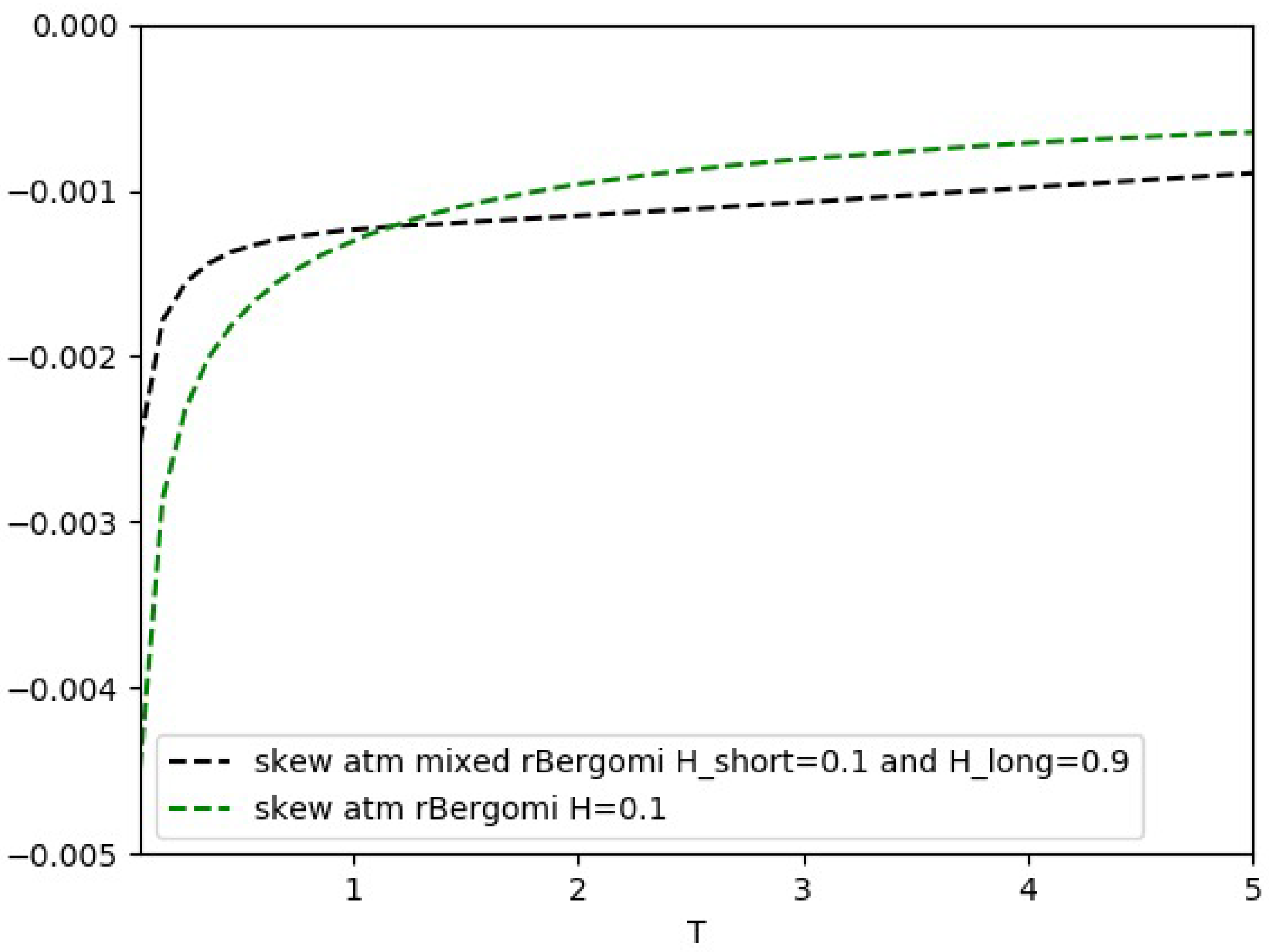
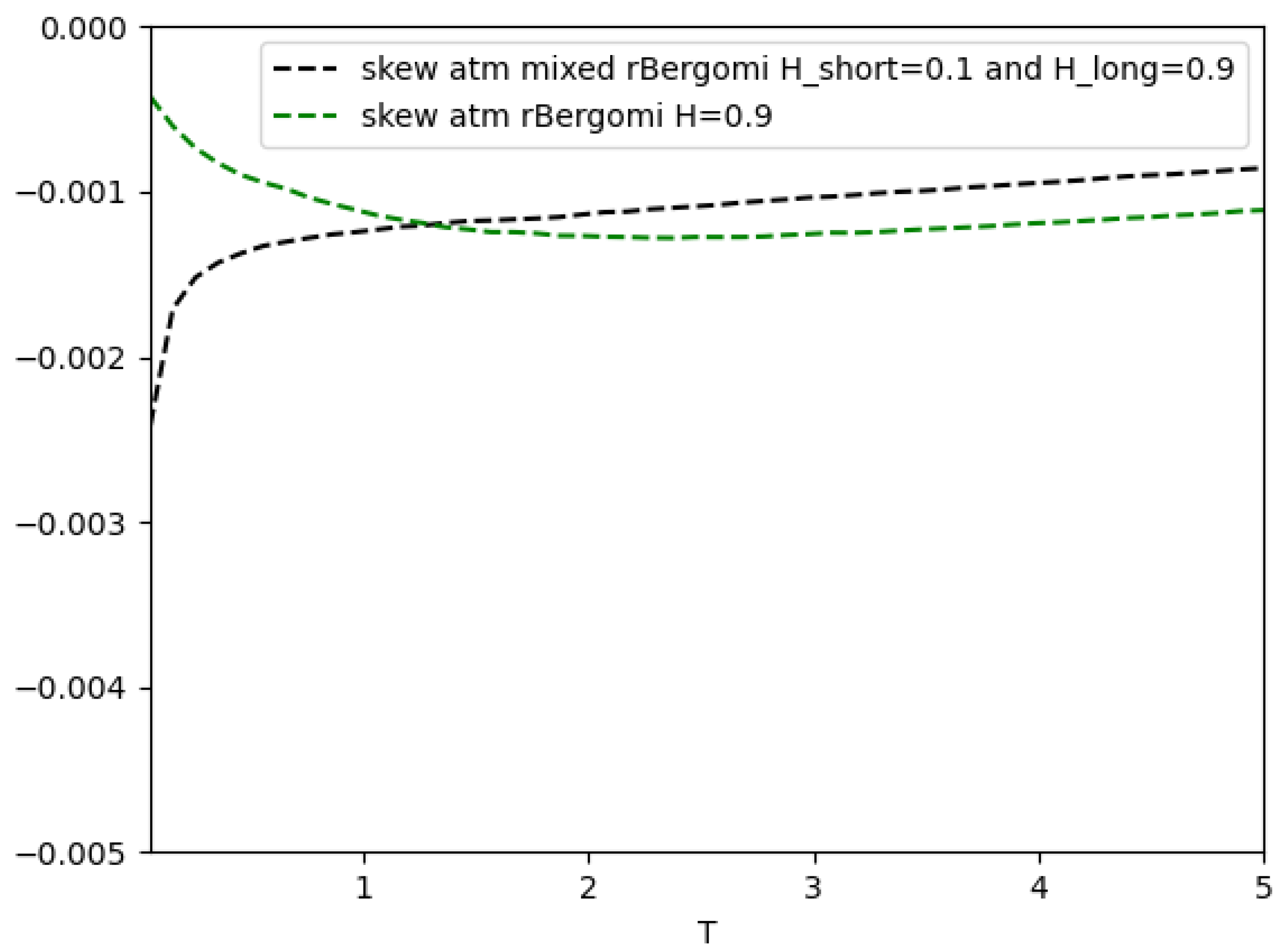
Let us observe this phenomenon in Figure 5 and Figure 6. In Figure 5, we show the ATM skew slope as a function of time to maturity for

• an mfBergomi model with $H=0.1$, $H^{\prime }=0.9$, ${\nu }_H={\nu }_{H^{\prime }}=0.5$, $\rho =-0.6$ and ${\sigma }_0^2=0.25$ and
• an rBergomi model with $H=0.1$, ${\nu }_H=0.5$, $\rho =-0.6$ and ${\sigma }_0^2=0.25$.

We see that both models have skew slopes that blow up at short maturities, but the decay (in absolute value) is slower for the mfBergomi.

We see that both models have a different short-term behavior. Note that the fBergomi model with $H>0.9$ increases the long-term skew, but it has no effect on the short end.

8. Conclusions

We showed that the fBm is a useful tool for modeling the long- and the short-term properties of the implied volatility surface because it allows us to increase the variability in the volatility both in short intervals (taking a Hurst parameter $H<\frac{1}{2}$) and in long intervals (taking $H>\frac{1}{2}$). This behavior is explicit in the short-end via Malliavin calculus techniques. The long- and short-memory properties of the volatility are not contradictory processes, as we showed in the numerical experiments. Fractional volatility models are more realistic volatility models. In particular, they can replicate the short-end blow-up of the empirical skew slope of the implied volatility. If we consider classical volatility models, where the volatility is a diffusion process, this phenomenon cannot be described and then the whole implied volatility surface cannot be calibrated. As a consequence, the classical methodology consists of calibrating the model for every fixed time to maturity, obtaining a different set of parameters for every maturity time. Fractional volatilities can be a first step in the simplification of calibration in real market practice. Moreover, we showed that fractional volatilities can be of interest in the joint modeling of the S&P index and the VIX, as well as other volatility indexes in the market such as the VSTOOXX and the OVX.

References

- Black, F.; Scholes, M. The pricing of options and corporate liabilities. J. Political Econ. 1973, 81, 637–654. [Google Scholar] [CrossRef] [Green Version]
- Renault, E.; Touzi, N. Option hedging and implied volatilities in a stochastic volatility model. Mat. Financ. 1996, 6, 279–302. [Google Scholar] [CrossRef]
- Stein, E.M.; Stein, J.C. Stock price distributions with stochastic volatility: An analytic approach. Rev. Financ. Stud. 1991, 4, 727–752. [Google Scholar] [CrossRef]
- Scott, L.O. Option pricing when the variance changes randomly: Theory, estimation and an application. J. Financ. Quant. Anal. 1987, 22, 419–438. [Google Scholar] [CrossRef]
- Hull, J.; White, A. The pricing of options on assets with stochastic volatilities. J. Financ. 1987, 42, 281–300. [Google Scholar] [CrossRef]
- Bates, D.S. Jumps and stochastic volatility: Exchange rate processes implicit in Deutsche Mark options. Rev. Financ. Stud. 1996, 9, 69–107. [Google Scholar] [CrossRef]
- Heston, S.L. A closed-form solution for options with stochastic volatility with applications to bond and currency options. Rev. Financ. Stud. 1993, 6, 327–343. [Google Scholar] [CrossRef] [Green Version]
- Johnson, H.; Shanno, D. Option pricing when the variance is changing. J. Financ. Quant. Anal. 1987, 22, 143–151. [Google Scholar] [CrossRef]
- Alòs, E.; León, J.A.; Vives, J. On the short-time behavior of the implied volatility for jump-diffusion models with stochastic volatility. Financ. Stoch. 2007, 11, 571–589. [Google Scholar] [CrossRef] [Green Version]
- Alòs, E. A generalization of the Hull and White formula with applications to option pricing approximation. Financ. Stoch. 2006, 10, 353–365. [Google Scholar] [CrossRef]
- Barndorff-Nielsen, O.E.; Shephard, N. Modelling by Lévy processes for Financial Econometrics. Lévy Process. Theory Appl. 2001, 283–318. [Google Scholar] [CrossRef]
- Barndorff-Nielsen, O.E.; Shephard, N. Econometric analysis of realized volatility and its use in estimating stochastic volatility models. J. R. Stat. Soc. Ser. Stat. Methodol. 2002, 64, 253–280. [Google Scholar] [CrossRef]
- Fouque, J.-P.; Papanicolaou, G.; Sircar, K.R.; Solna, K. Maturity cycles in implied volatility. Financ. Stoch. 2004, 8, 451–477. [Google Scholar] [CrossRef] [Green Version]
- Itô, K. Differential equations determining a Markoff process. In Japanese. J. Pan-Jpn. Math. Coll. 1942, 1077, 1352–1400. [Google Scholar]
- Doukhan, P.; Oppenheim, G.; Taqqu, M. Theory and Applications of Long-Range Dependence; Birkhäuser: Basel, Switzerland, 2003. [Google Scholar]
- Greene, M.T.; Fielitz, B.D. Long-term dependence in common stock returns. J. Financ. Econ. 1977, 4, 339–349. [Google Scholar] [CrossRef]
- Mandelbrot, B.B.; Wallis, J.R. Computer experiments with fractional Gaussian noises. Water Resour. 1969, 5, 228–267. [Google Scholar] [CrossRef]
- Mandelbrot, B.B. Fractals and Scaling in Finance: Discontinuity, Concentration, Risk; Springer: Berlin/Heidelberg, Germany, 1997. [Google Scholar]
- Mandelbrot, B.B.; Wallis, J.R. Some long-run properties of geophysical records. Water Resour. Res. 1969, 5, 321–340. [Google Scholar] [CrossRef] [Green Version]
- Comte, F.; Renault, E. Long memory in continuous-time stochastic volatility models. Mathematical Finance. Int. J. Math. Stat. Financ. Econ. 1998, 8, 291–323. [Google Scholar]
- Gatheral, J.; Jaisson, T.; Rosenbaum, M. Volatility is rough. Quant. Financ. 2018, 18, 933–949. [Google Scholar] [CrossRef]
- Roger, L.C.G. Arbitrage with fractional Brownian motion. Math. Financ. 1997, 7, 95–105. [Google Scholar] [CrossRef] [Green Version]
- Alòs, E.; León, J.A.; Nualart, D. Stochastic Stratonovich calculus for fractional Brownian motion with Hurst parameter less than 1/2. Taiwan J. Math. 2001, 5, 609–632. [Google Scholar] [CrossRef]
- Biagini, F.; Hu, Y.; Øksendal, B.; Zhang, T. Stochastic Calculus for Fractional Brownian Motion and Applications; Springer: Berlin/Heidelberg, Germany, 2008. [Google Scholar]
- León, J.A. Stratonovich type integration with respect to fractional Brownian motion with Hurst parameter less than 1/2. Bernoulli 2020, 26, 2436–2462. [Google Scholar] [CrossRef]
- León, J.A.; Nualart, D. An extension of the divergence operator for Gaussian processes. Stoch. Process. Their Appl. 2005, 115, 481–492. [Google Scholar] [CrossRef] [Green Version]
- Nualart, D. Stochastic integration with respect to fractional Brownian motion and applications. Contemp. Math. 2003, 336, 3–39. [Google Scholar]
- Nualart, D.; Tindel, S. A construction of the rough path above fractional Brownian motion using Volterra’s representation. Ann. Probab. 2011, 39, 1061–1096. [Google Scholar] [CrossRef]
- Mishura, Y. Stochastic Calculus for Fractional Brownian Motion and Related Processes; Springer: Berlin/Heidelberg, Germany, 2008. [Google Scholar]
- Zähle, M. Integration with respect to fractal functions and stochastic calculus I. Probab. Theory Relat. Fields 1998, 111, 333–374. [Google Scholar] [CrossRef]
- Kolmogorov, A.N. Wienersche Spiralen und einige andere interessante Kurven im Hilbertschen Raum. C.R. (Doklady). Acad. Sci. URSS (N.S.) 1940, 26, 115–118. [Google Scholar]
- Mandelbrot, B.B.; van Ness, J.W. Fractional Brownian motions, fractional noises and applications. SIAM Rev. 1968, 10, 422–437. [Google Scholar] [CrossRef]
- Molchan, G.; Golosov, J. Gaussian stationary processes with asymptotic power spectrum. Sov. Math. Dokl. 1969, 10, 134–137. [Google Scholar]
- Decreusefond, L.; Üstünel, A.S. Stochastic analysis of the fractional Brownian motion. Potential Anal. 1999, 10, 177–214. [Google Scholar] [CrossRef]
- Norros, I.; Valkeila, E.; Virtamo, J. An elementary approach to a Girsanov formula and other analytical results on fractional Brownian motions. Bernoulli 1999, 5, 571–587. [Google Scholar] [CrossRef]
- Lifshits, M.; Simon, T. Small deviations for fractional stable processes. In Annales de l’IHP Probabilités et Statistiques; Institut Henri Poincaré: Paris, France, 2005; Volume 41, pp. 725–752. [Google Scholar]
- Alòs, E.; García-Lorite, D. Malliavin Calculus in Finance: Theory and Practice; CRC Press: Boca Raton, FL, USA, 2021. [Google Scholar]
- Bayer, C.; Friz, P.; Gatheral, J. Pricing under rough volatility. Quant. Financ. 2016, 16, 887–904. [Google Scholar] [CrossRef]
- Euch, O.E.; Rosenbaum, M. Perfect hedging in rough Heston models. Ann. Appl. Probab. 2018, 28, 3813–3856. [Google Scholar] [CrossRef] [Green Version]
- Malliavin, P. Stochastic calculus of variations and hypoelliptic operators. In Proceedings of the International Symposium on Stochastic Differential Equations; Kyoto 1976, 195–263; Academic Press: Cambridge, MA, USA, 1978. [Google Scholar]
- Malliavin, P.; Thalmaier, A. Stochastic Calculus of Variations in Mathematical Finance; Springer: Berlin/Heidelberg, Germany, 2006. [Google Scholar]
- Nunno, G.D.; Øksendal, B.; Proske, F. Malliavin Calculus with Applications to Finance; Springer: Berlin/Heidelberg, Germany, 2009. [Google Scholar]
- Gaveau, B.; Trauber, P. L’intégrale stochastique comme opérateur de divergence dans l’space fonctionnel. J. Funct. Anal. 1982, 46, 230–238. [Google Scholar] [CrossRef] [Green Version]
- Skorohod, A.V. On a generalization of a stochastic integral. Theory Probab. Its Appl. 1975, 20, 219–233. [Google Scholar] [CrossRef]
- León, J.A.; Navarro, R.; Nualart, D. An anticipating calculus approach to the utility maximization of an insider. Math. Financ. 2003, 13, 171–185. [Google Scholar] [CrossRef]
- Nualart, D. The Malliavin Calculus and Related Topics, 2nd ed.; Springer: Berlin/Heidelberg, Germany, 2006. [Google Scholar]
- Clark, J.M.C. The representation of functionals of Brownian motion by stochastic integrals. Ann. Math. Stat. 1970, 41, 1282–1295. [Google Scholar] [CrossRef]
- Haussmann, U.G. On the integral representation of functionals of Itô processes. Stochastics 1979, 3, 17–27. [Google Scholar] [CrossRef]
- Ocone, D. Malliavin’s calculus and stochastic integral representation of functional diffusion processes. Stochastics 1984, 12, 161–185. [Google Scholar] [CrossRef]
- Karatzas, I.; Ocone, D.L.; Li, J. An extension of Clark’s formula. Stoch. Stoch. Rep. 1991, 37, 127–131. [Google Scholar] [CrossRef]
- Ocone, D.L.; Karatzas, I. A generalized Clark representation formula, with applications to optimal portfolios. Stoch. Stoch. Rep. 1991, 34, 187–220. [Google Scholar] [CrossRef]
- Nualart, D.; Pardoux, E. Stochastic calculus with anticipating integrands. Probab. Th. Rel. Fields 1988, 78, 535–581. [Google Scholar] [CrossRef]
- Nualart, D. Analysis on Wiener space and anticipating stochastic calculus. In École d’été de Probabilités de Saint Flour XXV, Lecture Notes in Mathematics; Springer: Berlin/Heidelberg, Germany, 1998; Volume 1690, pp. 123–227. [Google Scholar]
- Fink, H. An arbitrage-free real-world model for fractional option prices. J. Deriv. Fall 2021. [Google Scholar] [CrossRef]
- Lee, R. Implied and local volatilities under stochastic volatility. Int. J. Theor. Appl. Financ. 2001, 4, 45–89. [Google Scholar] [CrossRef] [Green Version]
- Cont, R.; Tankov, P. Financial Modelling with Jump Processes; CRC Press: Boca Raton, FL, USA, 2004. [Google Scholar]
- Fouque, J.-P.; Papanicolaou, G.; Sircar, K.R. Derivatives in Financial Markets with Stochastic Volatility; Cambridge University Press: Cambridge, UK, 2000. [Google Scholar]
- Alòs, E.; García-Lorite, D.; Muguruza, A. On smile properties of volatility derivatives and exotic products: Understanding the VIX skew. arXiv 2018, arXiv:1808.03610. [Google Scholar]
- Gatheral, J.; Jusselin, P.; Rosenbaum, M. The quadratic rough Heston model and the joint S&P 500/VIX smile calibration problem. arXiv 2020, arXiv:2001.01789. [Google Scholar]
- Romano, M.; Touzi, N. Contingent claims and market completeness in a stochastic volatility model. Math. Financ. 1997, 7, 399–412. [Google Scholar] [CrossRef]
- Willard, G.A. Calculating prices and sensitivities for path-independent securities in multifactor models. J. Deriv. 1997, 5, 45–61. [Google Scholar] [CrossRef]
- Solé, J.L.; Utzet, F.; Vives, J. Canonical Lévy process and Malliavin calculus. Stoch. Process. Their Appl. 2007, 117, 165–187. [Google Scholar] [CrossRef] [Green Version]
- Alòs, E.; León, J.A.; Pontier, M.; Vives, J. A Hull and White formula for a general stochastic volatility jump-diffusion model with applications to the study of the short-time behaviour of the implied volatility. J. Appl. Math. Stoch. Anal. 2008, 359142. [Google Scholar] [CrossRef] [Green Version]
- Medvedev, A.; Scaillet, O. Approximation and calibration of short-term implied volatilities under jump-diffusion stochastic volatility. Rev. Financ. Stud. 2007, 20, 427–459. [Google Scholar] [CrossRef] [Green Version]
- Jafari, H.; Vives, J. A Hull and White formula for a stochastic volatility Lévy model with infinite activity. Commun. Stoch. Anal. 2013, 7, 321–336. [Google Scholar] [CrossRef] [Green Version]
- Alòs, E.; León, J.A. On the short-maturity behaviour of the implied volatility skew for random strike options and applications to option pricing approximation. Quant. Financ. 2016, 16, 31–42. [Google Scholar] [CrossRef]
- Alòs, E.; Jacquier, A.; León, J.A. The implied volatility of Forward-Start options: ATM short-time level, skew and curvature. Stochastics 2019, 91, 37–51. [Google Scholar] [CrossRef] [Green Version]
- Merino, R.; Vives, J. Option price decomposition in spot-dependent volatility models and some applications. Int. J. Stoch. Anal. 2017, 2017, 8019498. [Google Scholar] [CrossRef] [Green Version]
- Alòs, E.; León, J.A. A note on the implied volatility of floating strike Asian options. Decis. Econ. Financ. 2019, 42, 743–758. [Google Scholar] [CrossRef]
- Alòs, E.; León, J.A. On the curvature on the smile in stochastic volatility models. SIAM J. Financ. Math. 2017, 8, 373–399. [Google Scholar] [CrossRef]
Figure 1.
Simulated fBm paths with , and .
Figure 2.
Simulated skews and smiles for a Heston model with , and
Figure 3.
Simulated similes for a Heston model with = 0.05, = 0.9, k = 3, = 0.8, = 0 and T = 0.1, 0.5, 1, and 5.
Figure 4.
Stock: Apple; expiration: 16 April 2010; data courtesy of Rafael De Santiago (IESE, Barcelona).
Figure 5.
Slope skew for an mfBergomi model and an rBergomi model with .
Figure 6.
Slope skew for an mfBergomi model and an fBergomi model with .
Publisher’s Note: MDPI stays neutral with regard to jurisdictional claims in published maps and institutional affiliations. |
© 2021 by the authors. Licensee MDPI, Basel, Switzerland. This article is an open access article distributed under the terms and conditions of the Creative Commons Attribution (CC BY) license (https://creativecommons.org/licenses/by/4.0/).
Share and Cite
MDPI and ACS Style
Alòs, E.; León, J.A. An Intuitive Introduction to Fractional and Rough Volatilities. Mathematics 2021, 9, 994. https://doi.org/10.3390/math9090994
AMA Style
Alòs E, León JA. An Intuitive Introduction to Fractional and Rough Volatilities. Mathematics. 2021; 9(9):994. https://doi.org/10.3390/math9090994
Chicago/Turabian StyleAlòs, Elisa, and Jorge A. León. 2021. "An Intuitive Introduction to Fractional and Rough Volatilities" Mathematics 9, no. 9: 994. https://doi.org/10.3390/math9090994
Note that from the first issue of 2016, this journal uses article numbers instead of page numbers. See further details here.