Equity Cost Induced Dichotomy for Optimal Dividends with Capital Injections in the Cramér-Lundberg Model

Abstract

We investigate a control problem leading to the optimal payment of dividends in a Cramér-Lundberg-type insurance model in which capital injections incur proportional cost, and may be used or not, the latter resulting in bankruptcy. For general claims, we provide verification results, using the absolute continuity of super-solutions of a convenient Hamilton-Jacobi variational inequality. As a by-product, for exponential claims, we prove the optimality of bounded buffer capital injections $(-a,0,b)$ policies. These policies consist in stopping at the first time when the size of the overshoot below 0 exceeds a certain limit a, and only pay dividends when the reserve reaches an upper barrier b. An exhaustive and explicit characterization of optimal couples buffer/barrier is given via comprehensive structure equations. The optimal buffer is shown never to be of de Finetti ($a=0$) or Shreve-Lehoczy-Gaver ($a=\infty$) type. The study results in a dichotomy between cheap and expensive equity, based on the cost-of-borrowing parameter, thus providing a non-trivial generalization of the Lokka-Zervos phase-transition Løkka-Zervos (2008). In the first case, companies start paying dividends at the barrier $b^{*}=0$, while in the second they must wait for reserves to build up to some (fully determined) $b^{*}>0$ before paying dividends.

1. Introduction

Motivation. Keeping shareholders satisfied while maintaining the company liquid enough constitutes the core of the control activity of reserves/risk processes. The rough idea is that one should intelligently balance return over invested capital (dividends) and replenishment by capital injections to insure the company’s robustness against claims. The easiest way to conceive such balance can roughly be stated as follows: when below low levels $-a\le 0$ (a acting as a maximally-admitted severity of ruin), reserve processes should be replenished by capital injections at some cost (hereafter, the unitary cost is denoted by $k\ge 1$), and when above high levels $b>0$, they should be taken out of the reserves as dividends–see for example [1,2] and the comprehensive book [3].

Historical overview. The first results tackling a related problem, due to de Finetti [4], concerned maximizing the expected value of the discounted cumulative dividends until the time of passage below a given level, called ruin. This can be seen as a particular case of the above-mentioned setting in which the cost of “borrowing” money is $k=\infty$ (or, equivalently, in which the maximal-targeted severity of ruin is $a=0$.

Next, Shreve, Lehoczky and Gaver (1984) [5] (with extra help from Coffman and Karatzas), introduced, for a state-dependent diffusion process, the dividends problem for the reflected process (RP). This consists in maximizing the functional

$$\left\{\begin{array}{c}J(x,\pi ):=E_x\left[{\int }_0^{\infty }{e}^{-qt}(\mathrm{d}{L}_t-k\mathrm{d}{I}_t)\right],k\ge 1,\hfill \\ \mathrm{under} \mathrm{the} \mathrm{state} \mathrm{constraint} X_t\ge 0\hfill \end{array}\right.$$

(1)

where

• x is the initial surplus;
• q is a discount factor;
• $L_t$ are the cumulative dividends;
• $I_t$ are the cumulative forced capital injections each time the process attempts to cross into $(-\infty ,0)$, and $k>1$ is a proportional cost for injecting capital;
• $X_t$ is the process modified by capital injections and dividends, and $\pi =(L_t,I_t)$.

They studied this objective (roughly corresponding to unrestricted maximal severity of ruin $a=\infty$), as well as the classic de Finetti dividends with absorption problem (AP), separately (and left many outstanding open problems behind). A complete solution for both of these problems (AP) and (RP) for spectrally negative Lévy processes was given in [6]—see also [7,8,9,10,11] for further developments. Note though that all these papers deal with forced bailouts. To our best knowledge, our paper hereafter seems to be the first to quantify the optimal buffer (severity of ruin) when bankruptcy should replace individual bailouts (to be fair, this possibility has been considered before, but without studying optimality—see for example [12]). For a different approach, quantifying the optimal policy under an expected total bailouts constraint, see [13].

The next important step was taken in [14] who compared the problems (AP), (RP) in a Brownian setting. The first was incorporated into the latter by adding the possibility of bankruptcy at ruin, i.e., of not systematically using capital injections. Their objective is to maximize, under the state constraint $X_t\ge 0$,

$$J(x,\pi ):=E_x\left[{\int }_0^{{\tau }_{0-}^{\pi }}{e}^{-qt}(\mathrm{d}{L}_t-k\mathrm{d}{I}_t)\right],$$

(2)

where ${\tau }_{0-}^{\pi }$ denotes a policy-dependent random time (which may be ∞) when the controlled process goes below the ruin threshold. This objective is fundamentally different from that adopted in the “Shreve, Lehoczky and Gaver literature” cited before. Now, capital injections will not only modify the dividend barrier level, but may also provoke bankruptcy; this happens only when k is big enough—the so called Lokka-Zervos alternative.

More precisely, let $V_D\left(x\right),V_k\left(x\right)$, denote the value functions of the (AP) and (RP) problems. [14] showed, by analyzing the corresponding HJB equation, that for Brownian motion surpluses there exists a critical cost $k_c$ such that one of the following strategies is optimal:

• $k<k_c⟹V_D\left(x\right)<V_k\left(x\right)$; the optimal policy is (RP), i.e., pay dividends at an upper barrier $b_k$ and always inject capital at 0, implying that bankruptcy never occurs;
• $k\ge k_c⟹V_D\left(x\right)\ge V_k\left(x\right)$; the optimal policy is (AP), i.e., pay dividends in order to reflect the surplus process at some upper barrier $b^{*}\ge 0$, and never inject capital.

We wish to emphasize that the analysis conducted strongly relies on an heuristic step in [14] (first paragraph on page 959 leading to the boundary condition ([14], 5.2)), used when formulating the HJB. Roughly speaking, by invoking the Markovian structure at $x=0$, it is argued that the value functions must either be 0, or have a derivative equal to k. Both these conditions fail to hold when one deals with Exponential Jumps—see Remark 14; this means that the Lokka-Zervos alternative holds for Brownian motion only because of the absence of jumps. Note that subsequently, ref. [15] showed that a similar Lokka-Zervos alternative holds for the Cramér-Lundberg process with exponential jumps, provided that one restricts from the start to either de Finetti or Shreve, Lehoczky and Gaver policies; as we know now, these are locally the worst possible policies.

Aim. Our paper focuses on the optimization of a criterion of type (2) in a Cramér-Lundberg framework without further assumptions on behavior of the value function at $x=0$. We seek a related dichotomy (hereafter referred to as Lokka-Zervos alternative) of optimal policies following the expensiveness of capital injections. Three points are of particular interest

• we prove the optimality of policies such as those described at the very beginning for which, in general, $a\notin \left\{0,\infty \right\}$ (i.e., de Finetti and Shreve, Lehoczky and Gaver policies fail to be optimal);
• the resulting value function is not of class $C^1$ at 0 (in the sense that its derivative does not exist at $x=0$ and, more, the right-hand derivative at 0 is not k as assumed, for Brownian claims, in [14], 5.2). This can be found in Remark 14 and it implies, in particular, that the verification Theorem 4 has to be given for absolutely-continuous functions. Working with super-solutions also explains the particular form of the Equation (8) on ${\mathbb{R}}_{-}$.
• the optimal parameters $a^{*}$ and $b^{*}$ are completely characterized by non-trivial equations and so is the alternative-inducing cost $k^{*}$.

Method. We have organized our paper around the classical guess and verify procedure for solving stochastic control problems:

• Guess a family of policies which yields the optimum for all possible values of the parameters, and compute its expected net present value (EPV) in terms of the $W,Z$ scale functions.

Our paper shows that optimality is achieved here via “bounded buffer capital injections” $(-a,0,b)$ policies, consisting in stopping at the first time when the size of the overshoot below 0 exceeds the limit a defined in Theorem 12. These policies turn out to work better than both the de Finetti and the Shreve, Lehoczky and Gaver policies, which are locally the worst possible choices!

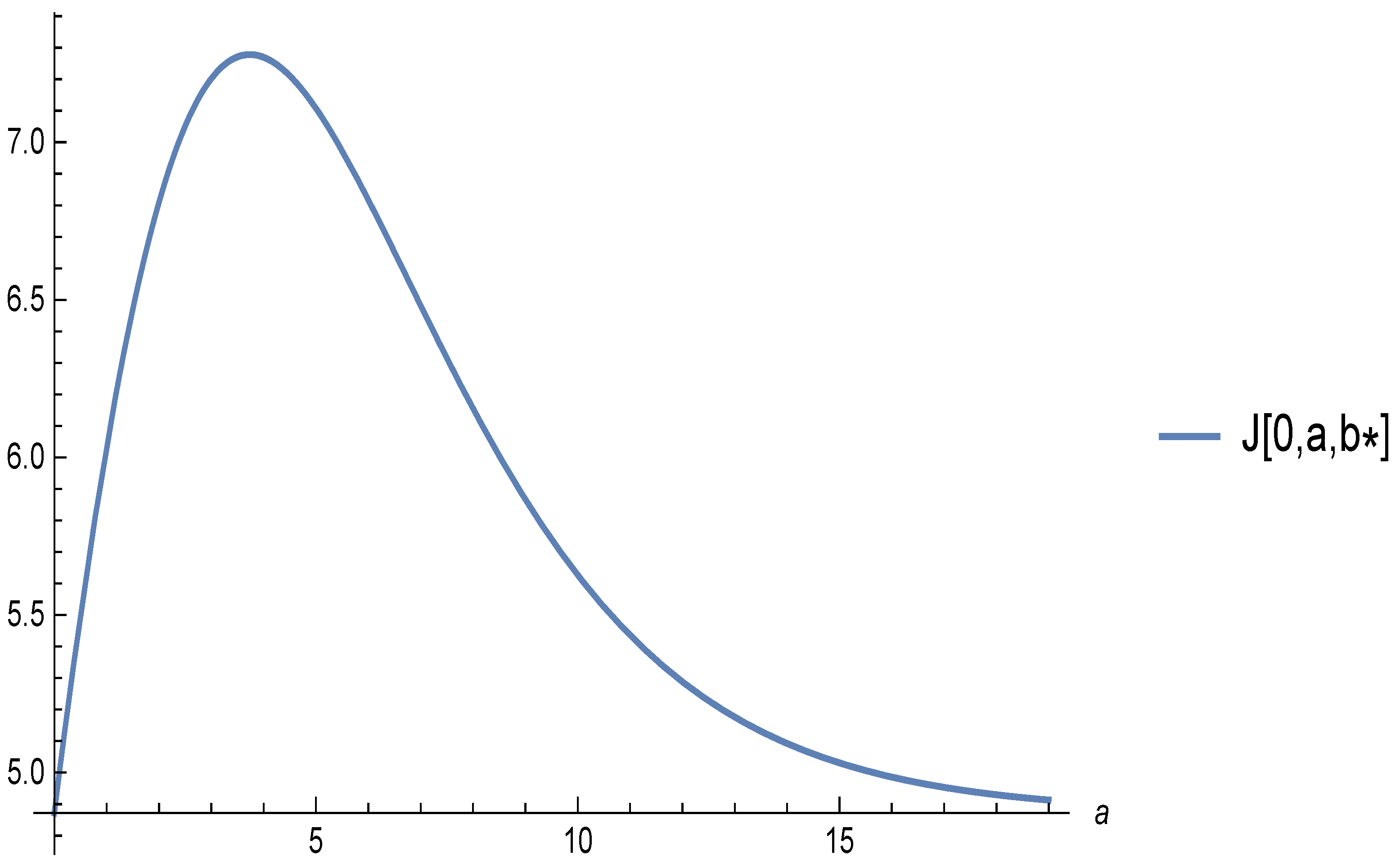
For example—see Figure 1, with a special choice $k=k_f\left(b^{*}\right)$ (see [15]) which ensures that the Shreve, Lehoczky and Gaver and de Finetti values coincide (with Exponential Jumps), the de Finetti and Shreve, Lehoczky and Gaver values are equal and globally the worst ones

$$\begin{array}{c}\hfill J_0^{a,b^{*}}>V_D\left(0\right)=V_k\left(0\right),\forall a>0.\end{array}$$

This illustrates the fact that the critical feature of our control problem is that capital injections should be allowed only when they are smaller than a critical size.

2.

Identify the optimal arguments with respect to the parameters of our policies. This step forced us to restrict to the case of exponential jumps, where the independence of ruin and ruin overshoots leads to simplifying factorizations related to the memoryless property of this distribution.

3.

In the final step, confirm the optimality of the selected candidate optimal policy via a verification theorem (sufficient condition for optimality). If the conjectured value function were sufficiently smooth (this means ${\mathcal{C}}^{\left(1\right)}$ in our problem), this would require only verifying that it satisfies an associated HJB equation (system of variational inequalities).

This is however not the case in our problem—see Remark 14 showing the value function to have a discontinuous derivative at 0—and made us turn to the minimality of the value functions among absolutely continuous super-solutions—see also the book [16] for a similar study (of the Cramér-Lundberg processwithout injections).

The model. We focus here on the classic Cramér-Lundberg model

$$X_t=x+pt-\sum _{i=1}^{N_t}{C}_i,p\ge 0,$$

(3)

with ${\left(C_i\right)}_{i\ge 1}$ being a family of i.i.d.r.v. distributed according to a distribution function F, and N being an independent Poisson process of intensity $\lambda >0$.

For optimization reasons, in the computations starting from Section 3 onward, F will be corresponding to the exponential law $\mathcal{E}xp\left(\mu \right)$, for some $\mu >0$. We restrict to this process since the independence of ruin and ruin overshoots leads to simpler formulae. Also, we take advantage of explicit computations in this case, which involve the two roots of the Cramér-Lundberg equation $\kappa \left(s\right)-q=0$ (where $\kappa \left(s\right)$ is the Laplace exponent ).

Remark 1.

The results in Section 2 may be modified to work for a considerably more general model of reserves with reinsurance

$$X_t=x+{\int }_0^t{p}^{r_s}\left(X_s\right)ds-\sum _{i=1}^{N_t}{r}_{{\tau }_i}\left(C_i\right),$$

where the premium p is (claim and) level-dependent in a Lipschitz manner and r is a further (continuous) control specifying the retention level for each claim. More precisely, we envisage $p^r\left(x\right):={\int }_{{\mathbb{R}}_{+}}p\left(y,x\right)d{F}^r\left(y\right)={\int }_{{\mathbb{R}}_{+}}p\left(r\left(y\right),x\right)F\left(dy\right)$, where y specifies the realised value of the claim C, $r\left(y\right)$ the retention level ($0\le r\left(y\right)\le y$) and F describes the distribution of claims C. The premium p is allowed to depend on the reserve x (e.g., in a linear way $p(y,x)=p_0\left(y\right)+p_1\left(y\right)x$ to recover Segerdahl’s model). However, for simplicity and consistency with the rest of the paper, only the Cramér-Lundberg case is presented below.

Related literature. Among other papers dealing with similar topics like [17,18,19], the most related to ours is [20], which was brought to our attention only after completion of our paper. Ref. [20] deals with the spectrally negative Lévy model, and the expressions for the cost functions provided in [20] are more general than ours. However, we prefer to offer here direct proofs adapted to the exponential case, for the sake of completeness.

Concerning optimality, the proof in [20] seems unclear to us, and we wrote two messages with no answer on this point to the authors. We believe that optimality is the hardest issue in our problem, and we have provided a full (and by no means easy) proof of that. In fact, this is precisely why we restricted to the exponential case; while the extension of the expected cost function to the matrix exponential case for example is standard—see (Section 7 in [21]), extending the optimality proof to the matrix exponential case seems very difficult and is for us still an open problem.

Note also (see Remark 1) that our approach in Section 2 may be modified to apply to more general spectrally negative processes, for example to the Segerdahl process [22], which is currently under study. Also importantly, for the Lévy case, our results are more explicit, and lead to algorithms presented in [21]. In fact, the algorithms (but not the optimality) are easily generalizable to the matrix-exponential case.

We end this literature review by mentioning a few related works on the dual spectrally positive Lévy model, where the situation is however much simpler, since capital injections occur without overshoot. A Lokka-Zervos alternative for the compound Poison model with exponential jumps and mixtures of exponential jumps was established in [23], and the first works on the general spectrally positive Lévy model were due to [24,25,26]. Note that in all these works the “overshoot dilemma” is absent: the dividends barrier may be overshot, but since we want to maximize dividends, in this case we do not need to distinguish between small and large overshoots.

Finally, we draw the attention to recent works concerning the diffusion approximation of the Cramér-Lundberg process, which further incorporate more sophisticated features like reinsurance [27,28,29]. It would be very interesting to investigate whether such sophisticated results can still be obtained while keeping the jumps.

Contents. The paper is organized as follows. Section 2 gives the necessary framework, mathematically formulates the admissible policies, the targeted cost and the value function. Section 2.2 turns to a structural study of the value function for arbitrarily distributed claims. This is achieved by making precise the regularity of the value function (Lipschitz-continuity, upper and lower-bounds in Proposition 2). Furthermore, the value function is characterized, among a class of linear-growth functions, as the smallest absolutely-continuous super-solution of the associated variational inequality of Hamilton-Jacobi integro-differential type. As it is by now standard, this characterization implies a verification result as to the optimality of policies (cf. Theorem 4).

The second part of the paper, starting with Section 3, is devoted to specifying the optimal policies in the exponential Cramér-Lundberg setting. We consider the costs associated to severity-constrained double barrier policies in Section 3.1. The explicit dependency on severity and upper barrier is made explicit in Propositon 7. The rigorous optimization on the two parameters is pursued in Section 4. The main result detailing the regions of optimality of the underlying parameters (cost of capital injections, severity of ruin and upper barrier) make the object of the main result Theorem 12. Finally, all the proofs are relegated to Section 6.

2. Optimizing Dividends and Capital Injections with Proportional Costs

2.1. The Framework

We will work with the process (3), living on a probability space $\left(\Omega ,\mathcal{F},\mathbb{P}\right)$ rich enough to support the family of i.i.d.r.v. ${\left(C_i\right)}_{i\ge 1}$ and the independent Poisson process N. The space is then endowed with the natural right-continuous, completed filtration $\mathbb{F}$. The surplus process will be modified by dividendsand capital injections (equity issuance), which are intended to maintain $X_t$ nonnegative.

• given a couple $\pi$: $=\left(L,I\right)$ describing dividends and capital injection, the modified surplus process is defined (under the ${\mathbb{P}}_x$) by setting

  $$X_t^{\pi }:=X_t-L_t+I_t;$$

  (4)
• the cumulative dividend strategy L is adapted, non-decreasing and càdlàg (right-continuous, left-limits), $L_{0-}=0$;
• the cumulative capital injection process I is adapted, non-decreasing and càdlàg, $I_{0-}=0$;
• the triplet $\pi :=\left(L,I\right)$ satisfying the previous conditions is referred to as (general) strategy and the family of all such strategies is denoted by ${\Pi }^{+}$.
  • (prior to ruin) for every $t\ge 0$, the dividends should satisfy

    $$△L_t:=L_t-L_{t-}\le X_{t-}^{\pi }-△{\overline{N}}_t+△I_t, \mathrm{where} {\overline{N}}_t:=\sum _{i=1}^{N_t}{C}_i.$$

    (5)
  • (after the ruin time $X_{t-}^{\pi }-△{\overline{N}}_t+△I_t<0$), we set $I_s=I_{t-},L_s=L_{t-},\forall s\ge t.$ (The reader is invited to note that in this case $t={\tau }_i$ one of the jumping times for N such that $I,L$ remain adapted, non-decreasing and càdlàg).
• the $\pi \in {\Pi }^{+}$ satisfying the dividends restriction is called an admissible strategy and the family of all such strategies is denoted by $\tilde{\Pi }\left(x\right)$.
• for an admissible strategy $\pi$,

  (a)

  we consider the ruin time ${\sigma }_{0-}^{x,\pi }:=inf\left\{t>0:X_{t-}^{\pi }-△{\overline{N}}_t+△I_t<0\right\}$ (if a “very large” claim occurs, bankruptcy is declared; as we will see in the main result, it is never optimal to take ${\sigma }_{0-}^{x,\pi }=\infty$ and modify the equity I accordingly).

  (b)

  the associated cost is

  $$\tilde{J}\left(x,\pi \right):={\mathbb{E}}_x[{\int }_{\left[0,{\sigma }_{0-}^{x,\pi }\right]}{e}^{-qt}\left(d{L}_s-kd{I}_s\right)],$$

  (6)

  (c)

  Every strategy $\pi$ can be replaced with $\tilde{\pi }$ by modifying $△{\tilde{I}}_t:=0$ if $X_{t-}^{\pi }-△{\overline{N}}_t+△I_t<0$ such that ${\sigma }_{0-}^{x,\pi }={\sigma }_{0-}^{x,\tilde{\pi }}$ and improving the associated cost $\tilde{J}\left(x,\pi \right)$. From now on, whenever a policy $\pi$ is considered, we identify it with $\tilde{\pi }$ and reason accordingly.

  (d)

  In connection to this type of policies and the related cost, we set

  $$\tilde{V}\left(x\right):=\underset{\pi \in \tilde{\Pi }\left(x\right)}{sup}\tilde{J}\left(x,\pi \right),x\in \mathbb{R}.$$

  (7)

2.2. The Value Function

We turn now to establishing a verification-type result for the stochastic control problem (7). Roughly speaking, we present the following program:

• First, we focus on the regularity properties of the value function $\tilde{V}$ (lower and upper-bound and Lipschitz-continuity) in Proposition 2.
• Second, we prove the connection between this value function and the associated partial-integral differential system (of HJB-type) in Proposition 3.
• Third, we show in Theorem 4 that the value function $\tilde{V}$ is the lowest absolutely-continuous super-solution of the associated equation and, as a verification result, give the optimality condition for candidate policies.

All the results in this section are valid for general laws of the claims C. To emphasize this, we consider that this law of C is given by its distribution function denoted by F.

2.3. Some Elementary Properties of the Value Function

We start with gathering some elementary properties of the value function

Proposition 2.

• For every $x\in {\mathbb{R}}_{+}$, the set of admissible strategies $\tilde{\Pi }\left(x\right)$ is non-empty. If $x,x^{\prime }\in {\mathbb{R}}_{+}$, then $\tilde{\Pi }\left(x\right)\subset \tilde{\Pi }\left(x^{\prime }\right)$ and, for every $\pi \in \tilde{\Pi }\left(x\right)$, ${\sigma }_{0-}^{x,\pi }\le {\sigma }_{0-}^{x^{\prime },\pi },\mathbb{P}-a.s.$.
• For every $x\ge 0$ and every $\pi \in \tilde{\Pi }\left(x\right)$, one has $\tilde{V}\left(x\right)\ge x+\frac{p}{\lambda +q}$.
• If $q>0$, then, for every $x\ge 0$ and every policy $\pi \in \tilde{\Pi }\left(x\right)$, one has $\tilde{J}(x,\pi )\le x+\frac{p}{q}$.
• For every $x\ge 0$ and every $\epsilon >0$, $\tilde{V}\left(x\right)+\epsilon \le \tilde{V}\left(x+\epsilon \right)\le \tilde{V}\left(x\right)+k\epsilon$.

The proof, relying on rather standard arguments, will be postponed to Section 6.

2.4. The HJB System

In connection to the value function $\tilde{V}$, we consider the following equation

$$\left\{\begin{array}{c}max\left\{\tilde{H}\left(x,\tilde{V},{\tilde{V}}^{\prime }\left(x\right)\right),1-{\tilde{V}}^{\prime }\left(x\right),{\tilde{V}}^{\prime }\left(x\right)-k\right\}=0,\forall x\in {\mathbb{R}}_{+}\hfill \\ min\left\{max\left\{1-{\tilde{V}}^{\prime }\left(x\right),{\tilde{V}}^{\prime }\left(x\right)-k\right\},\tilde{V}\left(x\right)\right\}=0,\forall x\in {\mathbb{R}}_{-}\hfill \end{array}\right.,$$

(8)

where the Hamiltonian $\tilde{H}$ is given by

$$\tilde{H}\left(x,\varphi ,a\right):=pa+\lambda {\int }_{\mathbb{R}}\varphi (x-y)dF\left(y\right)-\left(q+\lambda \right)\varphi \left(x\right).$$

(9)

On ${\mathbb{R}}_{+}$, it is expected that the value function satisfy the first equation. The lower bound on the derivative (1) is linked to the possibility of lump-sum dividend payments, and the k upper bound is linked to the possibility of lump-sum, instant reserves replenishment. The second equation is written in prevision of a super-solution formulation. Indeed, a (non-negative) super-solution is expected to comply to the inequality ≤. In particular, either the derivative belongs to $[1,k]$, or the sub-solution has reached 0. As anticipated, here is the simplest link to our stochastic control problem:

Proposition 3.

The value function $\tilde{V}$ in (7) is an $\mathcal{AC}$ super-solution of (8).

The proof—postponed to Section 6—relies, as it usually does, on the dynamic programming principle. The absolute continuity of $\tilde{V}$ allows to obtain the desired properties on the derivative almost surely.

2.5. The Value Function as Smallest $\mathcal{AC}$ Super-Solution

In this section, we strive to characterize the value function $\tilde{V}$ as the smallest super-solution in the class of regular ($\mathcal{AC}$ i.e., absolutely continuous) functions with linear growth. We begin with the following (standard) approximating result. Let us point out that whenever $\varphi$ is a non-negative $\mathcal{AC}$ super-solution of (8), there exists a (unique) point $a_{\varphi }\le 0$ such that

$$\begin{array}{c}\hfill \varphi \left(x\right)=0,\forall x\le a_{\varphi },\varphi \left(x\right)>0,\forall x>a_{\varphi },{\varphi }^{\prime }\left(x\right)\in \left[1,k\right],\mathcal{L}eb-\mathrm{a}.\mathrm{s}.\mathrm{on} \left[a_{\varphi },\infty \right).\end{array}$$

(10)

As a consequence, we get the following result.

Theorem 4.

• The value function $\tilde{V}$ is non-negative, $x+\frac{p}{\lambda +q}\le \tilde{V}\left(x\right)\le x+\frac{p}{q},$ for $x\ge 0$ and $\tilde{V}\left(x\right)=max\left\{\tilde{V}\left(0\right)+kx,0\right\},\forall x\le 0$.
• Every non-negative $\mathcal{AC}$-regular of growth $\varphi \left(x\right)\le max\left\{x+\alpha ,0\right\}$ viscosity super-solution of (8), where α is introduced in Proposition 15, is greater than or equal to $\tilde{V}$ on ${\mathbb{R}}_{+}$.
• If ${\pi }^{*}:=\left({\pi }^x={\left(L,I\right)}^x\in \tilde{\Pi }\left(x\right),x\ge 0\right)$ is a family of admissible strategies such that the associated costs $\tilde{J}(·,{\pi }^{*})$ is an $\mathcal{AC}$ super-solution for (8), then ${\pi }^{*}$ is optimal and $\tilde{V}\left(x\right)=\tilde{J}(x,{\pi }^{*}),\forall x\in {\mathbb{R}}_{+}$.

The proof, again postponed to Section 6, is obtained in two steps. First, in order to prove the second assertion, we provide convenient approximations of $\varphi$ by a sequence ${\varphi }_n$ of convoluted (mollified) functions. Second, we conclude by proving that ${\varphi }_n$ are, up to an $n^{-1}$-controlled error, super-solutions of $\mathcal{L}{\varphi }_n\le 0$. The verification part (assertion 3) is a mere consequence of the previous comparison and the definition of $\tilde{V}$.

Remark 5.

Without any changes it can be shown that if ϕ is an $\mathcal{AC}$ super-solution of (8) on $\left(0,a\right)$, then, for every $x<a$ and every admissible policy π keeping $X^{\pi }<a$, the associated cost $J\left(x,\pi \right)\le \varphi \left(x\right)$.

3. The Value Function for the Cramér-Lundberg Model

3.1. The Guess Step: Severity-Constrained Double Barrier Policies, for the Cramér-Lundberg Process with Exponential Jumps

Now, we turn to the guess step of the “guess-and-verify” method, by computing the value function associated to $(a,b)$ policies consisting in injecting capital up till the level 0, provided that the severity of ruin does not exceed $a\ge 0$ and paying dividends as soon as the process reaches some upper level $b\ge 0$.

We recall that the modern control theory of spectrally negative Lévy processes uses intensively the so-called $W_q$ and $Z_q$ scale functions, defined respectively for $x\ge 0,q\ge 0$ as:

• the inverse Laplace transform of $\frac{1}{\kappa \left(s\right)-q}$, where $\kappa \left(s\right)$ is the Laplace exponent, and
• $Z_q\left(x\right)=1+q{\int }_0^x{W}_q\left(y\right)dy$.

The reader is referred to the papers [30,31,32] for the first appearance of these functions, and to [2,33,34] for extensive reviews. A further important role in the results below will be played by the functions

$$C_q\left(x\right)=p{W}_q\left(x\right)-Z_q\left(x\right),\forall x\ge 0$$

(11)

and

$$\left\{\begin{array}{c}S(s,x)=e^{-\mu s}{C}_q\left(x\right)+Z_q\left(x\right)\hfill \\ G(s,x)=m\left(s\right)C_q\left(x\right)\hfill \end{array}\right.,\forall s\ge 0,x\ge 0.$$

(12)

Here,

$$m\left(s\right)={\int }_0^{s}y\mu e^{-\mu y}\mathrm{d}y=\frac{1-e^{-\mu s}(\mu s+1)}{\mu },$$

(13)

denotes the mean function of our claims cut at level $s\ge 0$.

The reader is invited to note that

$$S(s,0)=1,C_q\left(0\right)=0=G(s,0),C_q^{\prime }(0+)=\frac{\lambda }{p},\forall s\ge 0,$$

and that $x\mapsto C_q\left(x\right),x\mapsto G(s,x),x\mapsto S(s,x)$ are non-decreasing functions (for all $s\ge 0$).

The Laplace exponent of the Cramér-Lundberg process with exponential jumps is $\kappa \left(s\right)=s\left(p-\frac{\lambda }{\mu +s}\right)$, and

$$\begin{array}{cc}\hfill W_q\left(x\right)& =\frac{\left({\Phi }_q+\mu \right)e^{{\Phi }_{q}x}-\left({\rho }_{-}+\mu \right)e^{{\rho }_{-}x}}{p\left({\Phi }_q-{\rho }_{-}\right)},x\ge 0,\hfill \end{array}$$

(14)

where ${\Phi }_q>0>{\rho }_{-}$ are the two roots of the second-order equation

$$p{\rho }^2+\left(p\mu -\lambda -q\right)\rho -\mu q=0.$$

The following proposition gathers a few results useful for explicit root computations (when $\sigma =0$).

Proposition 6.

The following assertions hold true simultaneously.

• ${\Phi }_q+{\rho }_{-}=-\frac{p\mu -\lambda -q}{p};{\Phi }_q{\rho }_{-}=-\frac{\mu q}{p}$;
• $p\rho \left(\rho +\mu \right)=\left(\lambda +q\right)\rho +\mu q,\rho \in \left\{{\Phi }_q,{\rho }_{-}\right\}$;
• ${\rho }_{-}+\mu \ge 0,\mathrm{and} p\left({\Phi }_q+\mu \right)\left({\rho }_{-}+\mu \right)=\lambda \mu$;
• $p{W}_q\left(x\right)-Z_q\left(x\right)=\frac{\lambda }{p\left({\Phi }_q-{\rho }_{-}\right)}\left(e^{{\Phi }_{q}x}-e^{{\rho }_{-}x}\right)\ge 0$, for all $x\ge 0$;
• For all $b\ge 0$, $W_q$ and $Z_q$ (extended by $W_q\left(x\right)=0,Z_q\left(x\right)=1,\forall x<0$) satisfy the equation $\mathcal{L}\varphi \left(b\right)=0$, where $\mathcal{L}$ is given by (41). More precisely,

  $$\begin{array}{cc}\hfill & p{W}_q^{\prime }(b+)+\lambda {\int }_0^b{W}_q\left(y\right)\mu e^{-\mu (b-y)}dy-\left(\lambda +q\right)W_q\left(b\right)=0;\\ & p{Z}_q^{\prime }(b+)+\lambda {\int }_{-\infty }^b{Z}_q\left(y\right)\mu e^{-\mu (b-y)}dy-\left(\lambda +q\right)Z_q\left(b\right)=0.\end{array}$$

Again, the essential elements of the (rather immediate) proof are postponed to Section 6.

Proposition 7.

For a perturbed Cramér-Lundberg process with exponential jumps, we let

$$J_x:=J^{a,b}\left(x\right):={\mathbb{E}}_x\left[{\int }_0^{{\sigma }_{0-}^{x,{\pi }^{a,b}}}{e}^{-qt}\left(d{L}_t-kd{I}_t\right)\right]$$

(15)

denote the expected discounted dividends and capital injections associated to policies ${\pi }^{a,b}$ consisting in capital injections with proportionality cost $k\ge 1$, provided that the severity of ruin is smaller than $a>0$ (and declaring bankruptcy for larger severity), and paying dividends as soon as the process reaches some upper level b. We set

$$z(a,J_0):={\int }_0^a(J_0-ky)\mu e^{-\mu y}\mathrm{d}y=J_0(1-e^{-\mu a})-km\left(a\right).$$

(16)

• The cost function satisfies, for $0\le x\le b$,

  $$J_x=\frac{W_q\left(x\right)}{W_q\left(b\right)}{J}_b+\left(Z_q\left(x\right)-\frac{W_q\left(x\right)}{W_q\left(b\right)}{Z}_q\left(b\right)\right)z\left(a,J_0\right).$$

  (17)
  In particular, if we set

  $$j_x:=J_x-z(a,J_0)Z_q\left(x\right),$$

  (18)
  then

  $$j_x=\frac{W_q\left(x\right)}{W_q\left(b\right)}{j}_b,0\le x\le b.$$

  (19)
• Moreover, the cost can be explicitly written as

  $$J_x=\left\{\begin{array}{cc}0\hfill & ,x<-a\hfill \\ kx+J_0,\hfill & ,x\in [-a,0]\hfill \\ kG(a,x)+J_{0}S(a,x)=kG(a,x)+\frac{1-k{\partial }_{b}G(a,b+)}{{\partial }_{b}S(a,b+)}S(a,x)\hfill & ,x\in [0,b]\hfill \end{array}\right.,$$

  (20)
  and

  $$J_0=\frac{1-k{\partial }_{b}G(a,b+)}{{\partial }_{b}S(a,b+)}=\frac{1-k[m\left(a\right)C_q^{\prime }(b+)]}{e^{-\mu a}{C}_q^{\prime }(b+)+q{W}_q\left(b\right)}.$$

  (21)

The proof is postponed to Section 6. The first assertion follows by applying, to the reserve process starting at $x\ge 0$, the strong Markov property at the time the process reaches either 0 or the upper barrier b. A second expression for $J_b^{a,b}$ can be obtained by looking at the behavior at the time of the first claim. As a consequence, we get the dependency $\left(a,b\right)\to J_0^{a,b}$.

Remark 8.

• The first step of the previous proposition applies also to the perturbed Cramér-Lundberg process obtained by adding a Brownian term $\sigma B_t$ to (3). The second and third however use specific features available only if $\sigma =0$ (in particular that $W_q\left(0\right)=\frac{1}{p}>0$).
• Note that

  $$(S\left(x\right),G\left(x\right))=\left\{\begin{array}{cc}(p{W}_q\left(x\right),0)\hfill & ,a=0\hfill \\ (Z_q\left(x\right),\frac{C_q\left(x\right)}{\mu })=(Z_q\left(x\right),Z_{q,1}\left(x\right))\hfill & ,a=\infty \hfill \end{array}\right.,$$

  (22)
  where the last identity $\frac{C_q\left(x\right)}{\mu }=Z_{q,1}\left(x\right)$ as well as the notation $Z_{q,1}$ appear in [15]. Our formula interpolates between the de Finetti and Shreve, Lehoczky and Gaver cases:

  $$J_x^{a,b}=\left\{\begin{array}{cc}{V}^{b]}\left(x\right):=\frac{W_q\left(x\right)}{W_q^{\prime }(b+)}\hfill & ,a=0\hfill \\ V_k^{b]}\left(x\right):=k{Z}_{q,1}\left(x\right)+Z_q\left(x\right)\frac{1-k{Z}_{q,1}^{\prime }\left(b\right)}{q{W}_q\left(b\right)}\hfill & ,a=\infty \hfill \end{array}\right..$$

  (23)
  (Again, for details, the reader is guided to [15] and references therein).
• The Equation (20) may also be expressed as

  $$J_x^{a,b}=\frac{S(a,x)}{{\partial }_{b}S(a,b+)}-k\left[{\partial }_{b}G(a,b+)\frac{S(a,x)}{{\partial }_{b}S(a,b+)}-G(a,x)\right],$$

  (24)

  and making $k=0$ shows that the expected discounted dividends are $\frac{S(a,x)}{{\partial }_{b}S(a,b+)}$. It follows that the expected capital injections when $k=1$ are ${\partial }_{b}G(a,b+)\frac{S(a,x)}{{\partial }_{b}S(a,b)}-{\partial }_{b}G(a,x+)$.

Remark 9.

Looking at the last case of the result (20) for our functional $J_x$, we notice formal similarities with the known particular cases $a=0,a=\infty$ (recalled in Remark 8).

To explain this, and to relate to other similar “case by case observations”, note first that our functional could be studied at three related levels: (A) stopping at $T=T_{-a}^{-}\wedge T_b^{+}$; (B) computing expected capital injections with reflection at T; (C) reflecting and getting dividends at T. The corresponding boundary conditions are $J_b=0,J_b^{\prime }=0,J_b^{\prime }=1$, and they will yield different formulas for $J_0$. We recall that the final corresponding results when $s=\infty$ are

$$\begin{array}{c}\hfill k\left(Z_{q,1}\left(x\right)-Z_q\left(x\right)\frac{Z_{q,1}\left(b\right)}{Z_q\left(b\right)}\right),k\left(Z_{q,1}\left(x\right)-Z_q\left(x\right)\frac{Z_{q,1}^{\prime }\left(b\right)}{Z_q^{\prime }\left(b\right)}\right),\\ \hfill k\left(Z_{q,1}\left(x\right)-Z_q\left(x\right)\frac{Z_{q,1}^{\prime }\left(b\right)}{Z_q^{\prime }\left(b\right)}\right)+\frac{Z_q\left(x\right)}{Z_q^{\prime }\left(b\right)}.\end{array}$$

Notice they are all decompositions into

• a term depending on b, which is multiplied by the scale function $Z_q\left(x\right)$, and
• a term independent of b, $Z_{q,1}\left(x\right)$, which has been called sometimes “smooth Gerber-Shiu function”—see for example [35], and also “smooth harmonic extension of $w\left(x\right)=x,x\le 0$, see [2]. It is striking that the scale function and the Gerber-Shiu function are the same for these three problems. This begs for a formula for the Gerber-Shiu function which does not depend on the problem, and such a candidate is offered by the “LRZ harmonic extension” obtained in [36,37]. However, this has only been rigorously proved in particular examples – see for example [12].

This informal discussion motivates us to call the functions $S,G$ the scale function and Gerber-Shiu function for our problem. For a more down to earth reason for this name, recall that $S,G$ interpolate between the de Finetti and Shreve, Lehoczky and Gaver scale function and Gerber-Shiu function, cf. (23).

4. The Optimal ${\mathit{a}}^{*},{\mathit{b}}^{*}$ for the Cramér-Lundberg Model with Exponential Claims

In the previous arguments, we found it convenient to express the cost $J^{a,b}\left(x\right)$ in terms of the functions S and G to illustrate computations starting from the fundamental scale functions $Z_q$ and $W_q$. From now on, however, instead of using this basis, we will switch to the fundamental exponentials $e^{{\Phi }_{q}x},{ϵ}^{{\rho }_{-}x}$ (see Proposition 6). With the notations

$$\gamma \left(x\right):=\frac{\left({\Phi }_q-{\rho }_{-}\right)}{{\Phi }_q{e}^{{\Phi }_{q}x}-{\rho }_{-}{e}^{{\rho }_{-}x}}\mathrm{and} \theta \left(x\right):=\frac{\left(e^{{\Phi }_{q}x}-e^{{\rho }_{-}x}\right)}{{\Phi }_q{e}^{{\Phi }_{q}x}-{\rho }_{-}{e}^{{\rho }_{-}x}},\forall x\ge 0,$$

(25)

(which lead to a separation of the variables $a,b$), the initial datum satisfies

$$J_0^{a,b}=\frac{p\gamma \left(b\right)-\lambda km\left(a\right)}{q+\mu q\theta \left(b\right)+\lambda e^{-\mu a}}.$$

(26)

4.1. Preliminary Remarks

We note first that $J_0^{a,\infty }\le 0$, and, thus, $b^{*}=\infty$ can never be optimal. For this purpose, one notes that ${lim}_{x\to \infty }\gamma \left(x\right)=0$. It follows that either $b^{*}=0$ or it is a critical point of $\left(0,\infty \right)\ni b\mapsto J_0^{a,b}$.

We start with a preparatory result, obtained by differentiating (21) with respect to a. For the complete proof, the reader is referred to Section 6.

Lemma 10.

The partial derivative of$J_0^{a,b}$with respect to a (on (0, ∞)) is given by

$$\begin{array}{ccc}& & \frac{\partial }{\partial a}{J}_0^{a,b}=\lambda \mu e^{-\mu a}\frac{-ak\left(q+\mu q\theta \left(b\right)\right)+p\gamma \left(b\right)+\lambda k\frac{e^{-\mu a}-1}{\mu }}{{\left(q+\mu q\theta \left(b\right)+\lambda e^{-\mu a}\right)}^2}.\hfill \end{array}$$

• As a consequence, picking $a\in \left\{0,\infty \right\}$ can never be optimal.
• For fixed$k\ge 1$ and $b\ge 0$, there exists a unique critical point $a_{k,b}\ne 0$ satisfying $\frac{\partial }{\partial a}{J}_0^{a_{k,b},b}=0.$

This is equivalent to

$$0=-k{a}_{k,b}\left(q+\mu q\theta \left(b\right)\right)+p\gamma \left(b\right)+\lambda k\frac{-1+e^{-\mu a_{k,b}}}{\mu }.$$

(27)

Furthermore, (27) implies that at $a_{k,b}$ our objective simplifies to

$$\begin{array}{ccc}\hfill & & J_0^{a_{k,b},b}=k{a}_{k,b}.\hfill \end{array}$$

Thus, the optimal policy can neither be of Shreve-Lehoczky-Gaver type (i.e., systematic injection to keep the reserve positive independently of the severity of the ruin), nor of De Finetti type.

We discover thus that our solution of the Lokka-Zervos problem provided in [15], where we restricted to these two types of policies, is irrelevant to the global optimization problem!

4.2. Determining the Candidate Maximal Arguments

Relying on the previous Lemma 10, we prove (see Section 6) the following characterization of overall optimal buffer and barrier.

Proposition 11.

If $(a^{*},b^{*})$ realizes the maximum of the quantity $J_0^{a,b}$, then

• either $b^{*}=0$, in which case (27) implies that $a^{*}=a_k:=a_{k,0}$ satisfies

  $$\begin{array}{c}\hfill -kq{a}_k+p+\lambda k\frac{-1+e^{-\mu a_k}}{\mu }=0;\end{array}$$

  (28)
• or $b^{*}\in \left(0,\infty \right)$ satisfies

  $$-\frac{p{\gamma }^{\prime }\left(b\right)}{\mu q{\theta }^{\prime }\left(b\right)}\left(q+\mu q\theta \left(b\right)\right)+p\gamma \left(b\right)+\lambda k\frac{-1+e^{-\frac{p{\gamma }^{\prime }\left(b\right)}{kq{\theta }^{\prime }\left(b\right)}}}{\mu }=0,{\gamma }^{″}\left(b\right)-\frac{{\gamma }^{\prime }\left(b\right)}{{\theta }^{\prime }\left(b\right)}{\theta }^{″}\left(b\right)\le 0,$$

  (29)
  $\frac{p{\gamma }^{\prime }\left(b\right)}{\mu q{\theta }^{\prime }\left(b\right)}>0,$ and

  $$a^{*}=\frac{p{\gamma }^{\prime }\left(b^{*}\right)}{k\mu q{\theta }^{\prime }\left(b^{*}\right)}.$$

  (30)

5. From Guess to Optimality

The main result in this paper is based on the verification Theorem 4. Using the guess step developed in the previous sections, we completely characterize the parameters k for which $b^{*}=0$, leading to a “take the money and run’ behavior at 0 and the remaining configurations, for which $b^{*}>0$. For each case, we show that the $(a^{*},b^{*}$)-policies (described in the guess step) induce an absolutely-continuous cost that is a super-solution of (8), thus being optimal.

Theorem 12.

 

A.

If ${\left(\lambda +q\right)}^2<\lambda p\mu$, then, we have the following dichotomy.

A1.

The “cheap” equity regime, with $b^{*}=0$, holds for $1\le k\le k^{*}$, where $k^{*}$ is the unique solution of

$$\begin{array}{cc}& \delta \left(k\right)=0,\mathrm{with} \left[1,\infty \right)\ni k\mapsto \delta \left(k\right):=\frac{\lambda +q}{\mu }+\lambda k\frac{-1+e^{-\frac{p\mu -\lambda -q}{qk}}}{\mu }.\hfill \end{array}$$

(31)

Here the strategy consists in injecting capital to take reserve to 0 (for levels above $-a_k$ satisfying (28)) and paying dividends with the barrier 0 (i.e., “take the money and run”) is optimal, and the optimal value function is

$$\tilde{V}\left(x\right)=k{\left(a_k+x\right)}^{+}{\mathbf{1}}_{x\le 0}+\left(x+k{a}_k\right){\mathbf{1}}_{x>0}.$$

A2.

For “expensive” equity i.e., $k>k^{*}$,

• The structure equation

  $$-\frac{p{\gamma }^{\prime }\left(b\right)}{\mu q{\theta }^{\prime }\left(b\right)}\left(q+\mu q\theta \left(b\right)\right)+p\gamma \left(b\right)+\lambda k\frac{-1+e^{-\frac{p{\gamma }^{\prime }\left(b\right)}{kq{\theta }^{\prime }\left(b\right)}}}{\mu }=0$$

  (32)

  admits at least one solution. Denote by $b^{*}$ the smallest solution of (32). Then, it holds that

  $$\begin{array}{c}\hfill a^{*}=\frac{p{\gamma }^{\prime }\left(b^{*}\right)}{k\mu q{\theta }^{\prime }\left(b^{*}\right)}.\end{array}$$

  (33)
• If $a_m$ designate the solutions of (28) (for $k=m$), then $a_k<a^{*}<a_1$.
• The strategy consisting in injecting capital to take reserve to 0 (for levels above $-a^{*}$ satisfying (33)) and paying dividends with the barrier $b^{*}$ is optimal. The optimal function is

  $$\begin{array}{c}\hfill \tilde{V}\left(x\right)=\left\{\begin{array}{cc}\hfill k{\left(a^{*}+x\right)}^{+},& \mathrm{if} x<0,\hfill \\ \hfill kG(a^{*},x)+k{a}^{*}S(a^{*},x),& \mathrm{if} x\in \left[0,b^{*}\right],\hfill \\ \hfill \tilde{V}\left(b^{*}\right)+x-b^{*},& \mathrm{if} x>b^{*},\hfill \end{array}\right.\end{array}$$

  (34)

B.

In the remaining case ${\left(\lambda +q\right)}^2\ge \lambda p\mu$, independently of $k\ge 1$, $b^{*}=0$ and the value function is got as in A1:

$$\tilde{V}\left(x\right)=k{\left(a_k+x\right)}^{+}{\mathbf{1}}_{x\le 0}+\left(x+k{a}_k\right){\mathbf{1}}_{x>0},$$

with $a_k$ given by the Equation (28).

Remark 13.

In preparation of the proof, the reader may want to note that (34) can be rewritten with the use of Proposition 6 (fourth assertion) as

$$kG(a^{*},x)+k{a}^{*}S(a^{*},x)=f_k\left(a^{*},a^{*}k,{\Phi }_q\right)e^{{\Phi }_{q}x}-f_k\left(a^{*},a^{*}k,{\rho }_{-}\right)e^{{\rho }_{-}x},$$

where

$$\left\{\begin{array}{c}m\left(r\right):=\frac{1-\left(r\mu +1\right)e^{-\mu r}}{\mu };g_k(r,J_0):=-J_0\left(1-e^{-\mu r}\right)+km\left(r\right);\hfill \\ f_k(r,J_0,\theta ):=\frac{\lambda g_k(r,J_0)+p{J}_0\left(\theta +\mu \right)}{p\left({\Phi }_q-{\rho }_{-}\right)}=J_0\frac{p\left(\theta +\mu \right)-\lambda \left(1-e^{-\mu r}\right)}{p\left({\Phi }_q-{\rho }_{-}\right)}+\frac{\lambda km\left(r\right)}{p\left({\Phi }_q-{\rho }_{-}\right)}.\hfill \end{array}\right.$$

As before, the proof is postponed to Section 6.

Remark 14.

 

• A careful look at the upper-bound in 2.2.2 (in the proof) shows that ${\tilde{V}}^{\prime }(0+)<k={\tilde{V}}^{\prime }(0-)$. As a consequence:
  • the heuristic intuition in ([14], 5.2) no longer holds true for our case ($\tilde{V}\left(0\right)>0$ and ${\tilde{V}}^{\prime }\left(0\right)=k$ fails to hold true);
  • $\tilde{V}$ is only absolutely continuous (but not $C^1$) such that the comparison in Theorem 4 must be given among absolutely continuous super-solutions.
• The equality in (50) gives a way to characterize $b^{*}$ when $\tilde{V}$ is known.

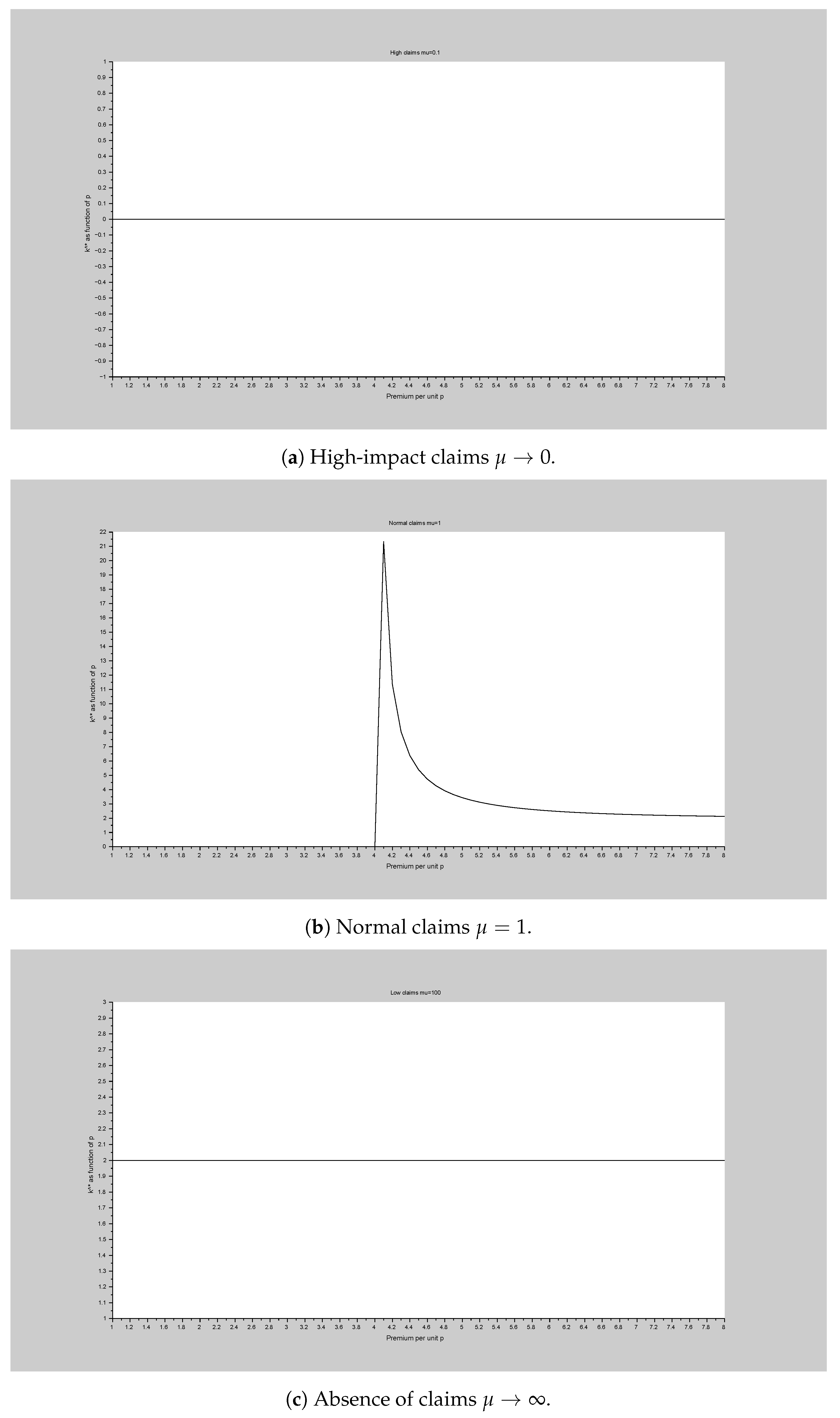
We illustrate the dependency of the discriminating equity level $k^{*}$ of $\mu$ and q in Figure 2.

• As $\mu \to 0$, the claims approach ∞ average. In a highly impacted market, the notion of equity expensiveness vanishes and it is not optimal to wait for any amount of time $b>0$ (Figure 2a).
• At the other end, as $\mu$ is large enough (Figure 2c), we are in a deterministic market which reaches an equilibrium separation of equities at $k^{*}=\frac{\lambda +q}{\lambda }$. A glance at (33) shows that, for expensive equity, there should be no capital injection.
• In between (Figure 2b), $k^{*}$ stabilizes to the equilibrium $\frac{\lambda +q}{\lambda }$ with large values of p. This is to be put in relation with the result in (Lemma 7 in [7]) giving a condition for $b^{*}=0$ (although the cited result does not consider buffered strategies).
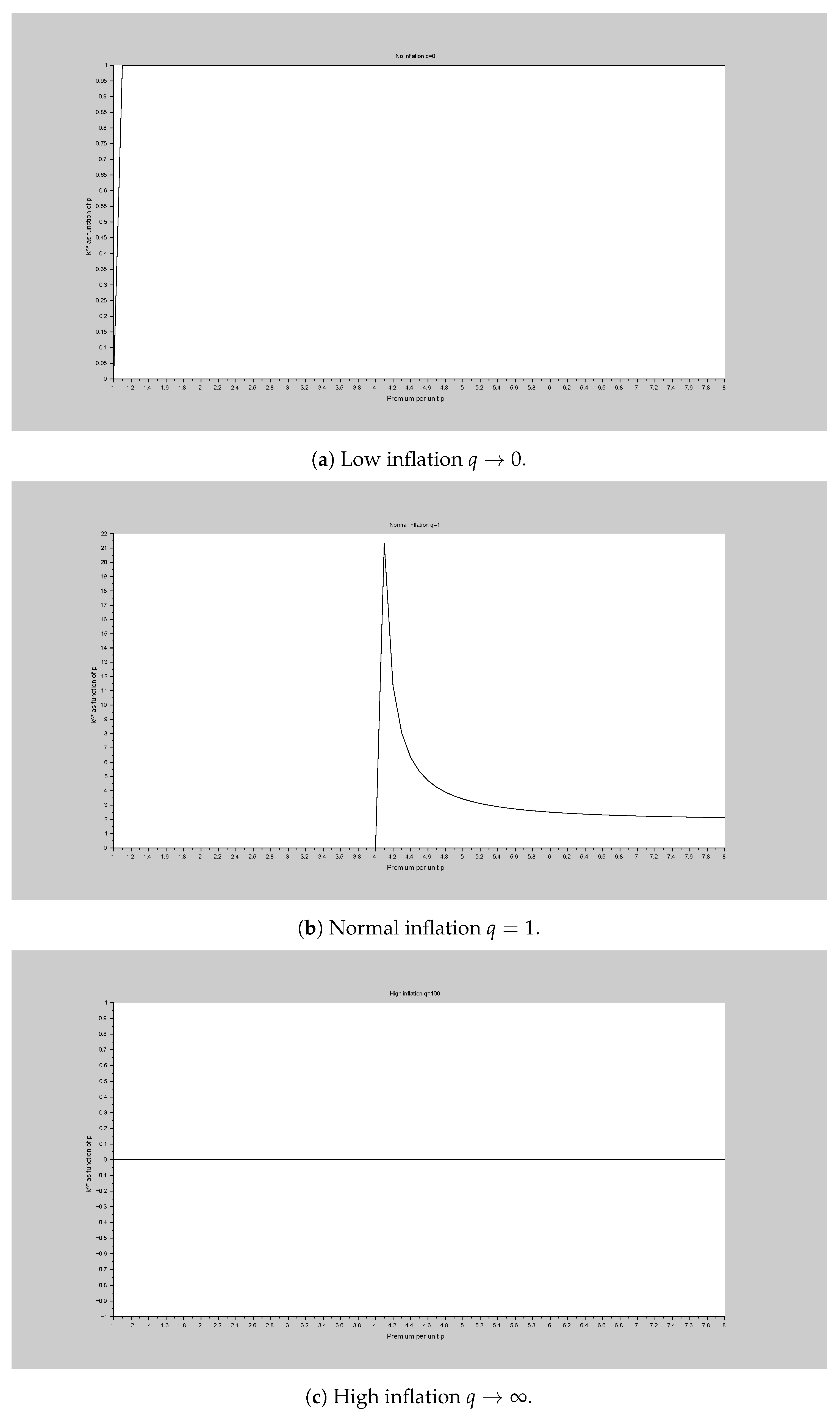
• On the other hand (Figure 3a), as the discount parameter $q\to 0+$, for all p that may give a dichotomy (cf. A), $p\mu -\lambda >0$ such that the Equation (31) leads to $k^{*}=1$. In other words, absence of inflation makes every equity $k>1$ expensive. Conversely (Figure 3c), high inflation (large q) makes the notion of equity expensiveness vanish.

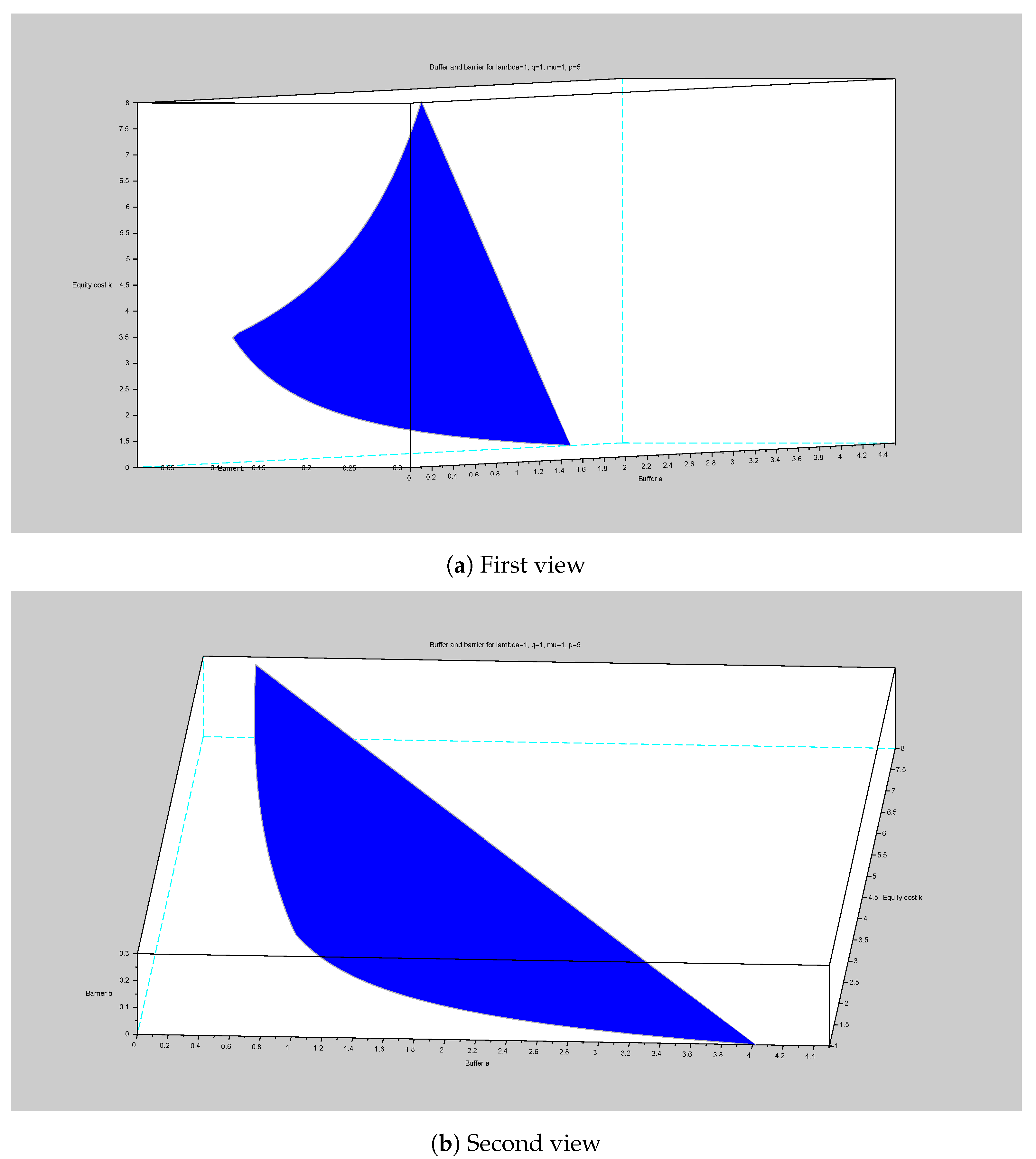
We end the section with a numerical illustration of the surface $(a^{*},b^{*})$ as the equity cost evolves in a compact interval in Figure 4.

A glance at the first point of view shows that $b^{*}=0$ until the critical value $k^{*}$ and then it increases with $k\ge k^{*}$. The second point of view shows a to be decreasing with the equity cost $k\le k^{*}$. Then, it continues decreasing, although somewhat slower with $k\ge k^{*}$.

6. Proofs of the Results

6.1. Proofs for the Value Function: Estimates, Dynamic Programming, Solution

Although following rather classical arguments, for our readers’ sake, we provide the proof of the basic properties of the value function $\tilde{V}$.

Proof of Proposition 2.

 

• The classical (no dividend, no injection) $\left(0,0\right)$ policy is an admissible strategy. The second result is a mere consequence of the definition of $X^{\pi }$.
• For $x\ge 0$, we consider the strategy consisting in no capital injection ($I=0$), then paying $L_0=x$ and (continuously) the premium and declare bankruptcy at the first (positive) claim. For this admissible strategy ${\pi }^0$, the ruin time ${\sigma }_{0-}^{x,{\pi }^0}={\tau }_1,\mathbb{P}-a.s.$ (the first jumping time except on the 0-probability event $C_1=0$). We have

  $$\tilde{V}\left(x\right)\ge \tilde{J}\left(x,{\pi }^0\right)=x+p\mathbb{E}[{\int }_0^{{\tau }_1}{e}^{-qt}dt]=x+\frac{p}{\lambda +q}.$$
• One merely notes that, for every $\pi \in \tilde{\Pi }\left(x\right)$,

  $$\left\{\begin{array}{cc}\hfill max\left\{X_{t-}^{\pi },0\right\}& \le x+pt+{\int }_{\left[0,t\right)}\left(d{I}_s-d{L}_s\right)\hfill \\ \hfill max\left\{X_t^{\pi },0\right\}& \le x+pt+{\int }_{[0,t]}\left(d{I}_s-d{L}_s\right)\hfill \end{array}\right.,\forall t\in \left[0,{\sigma }_{0-}^{x,\pi }\right],\mathbb{P}-a.s.,$$

  (35)

  on $\left\{{\sigma }_{0-}^{x,\pi }<\infty \right\}$. Then,

  $${\int }_{[0,{\sigma }_{0-}^{x,\pi }}]e^{-qs}\left(d{L}_s-kd{I}_s\right)\le {\int }_{\left[0,{\sigma }_{0-}^{x,\pi }\right]}{e}^{-qs}\left(d{L}_s-d{I}_s\right)\le x+\frac{p}{q},{\mathbb{P}}_x-a.s.$$

  (36)

The conclusion follows by computing the average under ${\mathbb{P}}_x$.

4.

The first inequality follows by modifying an arbitrary strategy $\pi \in \tilde{\Pi }\left(x\right)$ into ${\pi }^{\epsilon }:=\left(L+\epsilon ,I\right)$ on ${\mathbb{R}}_{+}$ to get ${\pi }^{\epsilon }\in \tilde{\Pi }\left(x+\epsilon \right)$. For the last inequality, one modifies (on ${\mathbb{R}}_{+}$) an admissible strategy $\pi \in \tilde{\Pi }\left(x+\epsilon \right)$ into ${\pi }_{\epsilon }:=\left(L,I+\epsilon \right)\in \tilde{\Pi }\left(x\right)$.

□

Let us now turn to the proof of the super-solution behavior of $\tilde{V}$.

Proof of Proposition 3.

Let $x\in \left(0,\infty \right)$.

As it is by now standard, the arguments rely on the dynamic programming principle (The proof of this principle is skipped in this paper. It is quite similar to the one without injections, e.g., in [16] with the only supplementary difficulty that $X^{\pi }$ is not bounded, due to the presence of the injection term I. However, this is overcome by restricting to 1-optimal policies as we did in the proof of Theorem 4 in order to obtain convenient bounds on the expected value of injections, hence of reserves. A paper on level-depending premiums and reinsurance is ongoing and the DPP is proven in this much more general framework) stating that, given a stopping time $\tau$,

$$\tilde{V}\left(x\right)=\underset{\pi \in \tilde{\Pi }\left(x\right)}{sup}{\mathbb{E}}_x\left[{\int }_{\left[0,\tau \wedge {\sigma }_{0-}^{x,\pi }\right]}{e}^{-qs}\left(d{L}_s-kd{I}_s\right)+e^{-q\left(\tau \wedge {\sigma }_{0-}^{x,\pi }\right)}\tilde{V}\left(X_{\tau \wedge {\sigma }_{0-}^{x,\pi }}\right)\right].$$

We consider the admissible strategy $\pi :=\left(0,0\right)$ (no dividends, no capital injection). We begin with the remark that, in this case,

$$X_s^{\pi }\le x+ps \mathrm{has} \mathrm{an} \mathrm{explicit} \mathrm{upper} \mathrm{bound}.$$

(37)

The dynamic programming principle (using the time of the first claim ${\tau }_1\le {\sigma }_{0-}^{x,\pi }$ and $t>0$, i.e., $\tau :={\tau }_1\wedge t$) with the particular choice of $\pi =(0,0)$ yields

$$\begin{array}{cc}\hfill \tilde{V}\left(x\right)& \ge {\mathbb{E}}_x[e^{-q\left(t\wedge {\tau }_1\right)}\tilde{V}\left(X_{t\wedge {\tau }_1}^{\pi }\right)]\hfill \\ \hfill & =e^{-qt}\tilde{V}\left(x+pt\right){\mathbb{P}}_x\left({\tau }_1>t\right)+{\mathbb{E}}_x{}_{[}{\mathbf{1}}_{{\tau }_1\le t}{e}^{-q{\tau }_1}\tilde{V}\left(X_{{\tau }_1}^{\pi }\right)]\hfill \\ \hfill & \ge e^{-qt}\tilde{V}\left(x+pt\right){\mathbb{P}}_x\left({\tau }_1>t\right)+{\mathbb{E}}_x[{\mathbf{1}}_{{\tau }_1\le t}{e}^{-q{\tau }_1}]{\int }_{{\mathbb{R}}_{+}}\tilde{V}(x-y)dF\left(y\right).\hfill \end{array}$$

(38)

by passing $\tilde{V}\left(x\right)$ on the right and dividing by t, it follows that

$$\begin{array}{cc}\hfill 0\ge & \frac{e^{-qt}\tilde{V}\left(x+pt\right){\mathbb{P}}_x\left({\tau }_1>t\right)-\tilde{V}\left(x\right)}{t}+\frac{\lambda }{\lambda +q}\frac{1-e^{-\left(\lambda +q\right)t}}{t}{\int }_{{\mathbb{R}}_{+}}\tilde{V}\left(x-y\right)dF\left(y\right)\hfill \\ \hfill =& \frac{{\int }_0^t\left(-(q+\lambda )e^{-(q+\lambda )s}\tilde{V}(x+ps)+e^{-(q+\lambda )s}p{\tilde{V}}^{\prime }(x+ps)\right)ds}{t}\hfill \\ \hfill & +\frac{\lambda }{\lambda +q}\frac{1-e^{-\left(\lambda +q\right)t}}{t}{\int }_{{\mathbb{R}}_{+}}\tilde{V}\left(x-y\right)dF\left(y\right).\hfill \end{array}$$

(39)

Passing $t\downarrow 0$, one gets

$$0\ge p{\tilde{V}}^{\prime }\left(x\right)+\lambda {\int }_{{\mathbb{R}}_{+}}\tilde{V}(x-y)dF\left(y\right)-(\lambda +q)\tilde{V}\left(x\right).$$

The Lipschitz estimates on $\tilde{V}$ take care of the bounds on the derivative.

For negative reserves $x<0$, only two strategies are possible: either declare immediate bankruptcy s.t. $\tilde{J}(x,\pi )=0$ or inject capital at unitary cost k leading to $\tilde{V}\left(x\right)={\left(\tilde{V}\left(0\right)+kx\right)}^{+}$. The super-solution condition follows. □

Before providing the proof of Theorem 4, we need the following approximation result.

Proposition 15.

Let ϕ be a non-negative $\mathcal{AC}$ super-solution of (8) s.t. $\varphi \left(y\right)\le y+\alpha$, for all $y\ge 0$ and some $\alpha \in \mathbb{R}$. Then, there exists a sequence of $C^1$ functions ${\varphi }_n$ s.t.

• $\varphi \left(x\right)\le {\varphi }_n\left(x\right)\le \varphi \left(x\right)+\frac{k}{n}$ on $\mathbb{R}$;
• ${\varphi }_n^{\prime }\in \left[1,k\right]$ on $\left[a_{\varphi },\infty \right)$;
• ${\displaystyle \underset{n\to \infty }{lim}}{\varphi }_n^{\prime }={\varphi }^{\prime }$ (pointwise a.e. on $\mathbb{R}$).

Proof. 

The proof is a mere modification of (Lemma 4.1 in [16]). Let us consider, for a sequence of standard mollifiers based on a non-negative continuously differentiable function $\rho$ supported on $(0,1)$ i.e, by setting ${\rho }_n\left(x\right):=n\rho \left(nx\right)$, the convoluted function

$${\varphi }_n\left(x\right):={\int }_{\left(0,\frac{1}{n}\right)}\varphi (x+s)n\rho \left(ns\right)ds,\forall n\ge 1.$$

It is clear that ${\varphi }_n$ are of class $C^1$, as are the convergence assertions. Since $\varphi$ is $\mathcal{AC}$, ${\varphi }^{\prime }\in \left[1,k\right],a.e.$ on $\left[a_{\varphi },\infty \right)$ which implies the same bounds on the ${\varphi }_n^{\prime }$. □

We proceed with the proof of the minimality of $\tilde{V}$ and the verification result for policies.

Proof of Theorem 4.

We fix $x\ge 0$. If $\varphi$ is a non-negative, $\mathcal{AC}$ super-solution of (8), then, using ${\varphi }_n$ introduced before and Itô’s formula, we get

$$\begin{array}{cc}& {\mathbb{E}}_x[e^{-q\left(t\wedge {\sigma }_{0-}^{x,\pi }\right)}{\varphi }_n\left(X_{t\wedge {\sigma }_{0-}^{x,\pi }}^{\pi }\right)]-{\varphi }_n\left(x\right)\hfill \\ \hfill \le & {\mathbb{E}}_x\left[{\int }_{\left[0,t\wedge {\sigma }_{0-}^{x,\pi }\right]}\left\{e^{-qs}\left(kd{I}_s-d{L}_s\right)+e^{-qs}\mathcal{L}{\varphi }_n\left(X_{s-}^{\pi }\right)ds\right\}\right],\hfill \end{array}$$

(40)

where

$$\mathcal{L}{\varphi }_n\left(y\right):=p{\varphi }_n^{\prime }\left(y\right)+\lambda {\int }_{{\mathbb{R}}_{+}}\left({\varphi }_n(y-z)-{\varphi }_n\left(y\right)\right)dF\left(z\right)-q{\varphi }_n\left(y\right).$$

(41)

If the strategy $\pi =\left(L,I\right)$ is 1-optimal for $\tilde{V}\left(x\right)$, then, owing to (35), one has

$$\begin{array}{c}\tilde{V}\left(x\right)-1\le \tilde{J}(x,\pi )\le {\mathbb{E}}_x[{\int }_{[0,t\wedge {\sigma }_{0-}^{x,\pi }]}{e}^{-qs}\left(d{L}_s-kd{I}_s\right)+e^{-q\left(t\wedge {\sigma }_{0-}^{x,\pi }\right)}\tilde{V}\left(X_{t\wedge {\sigma }_{0-}^{x,\pi }}^{\pi }\right)]\hfill \\ \le {\mathbb{E}}_x\left[{\int }_{[0,t\wedge {\sigma }_{0-}^{x,\pi }]}{e}^{-qs}\left(d{L}_s-d{I}_s\right)+e^{-q\left(t\wedge {\sigma }_{0-}^{x,\pi }\right)}\left(max\left\{X_{t\wedge {\sigma }_{0-}^{x,\pi }}^{\pi },0\right\}+\frac{p}{q}\right)\right]\hfill \\ -(k-1){\mathbb{E}}_x\left[{\int }_{\left[0,t\wedge {\sigma }_{0-}^{x,\pi }\right]}{e}^{-qs}d{I}_s\right]\hfill \\ \le x+\frac{2p}{q}-(k-1){\mathbb{E}}_x\left[{\int }_{\left[0,t\wedge {\sigma }_{0-}^{x,\pi }\right]}{e}^{-qs}d{I}_s\right].\hfill \end{array}$$

(42)

It follows that

$${\mathbb{E}}_x[{\int }_{\left[0,{\sigma }_{0-}^{x,\pi }\right]}{e}^{-qs}d{I}_s]\le \frac{1}{k-1}\left(x+\frac{2p}{q}+1-\tilde{V}\left(x\right)\right)\le \frac{1}{k-1}\left(\frac{2p}{q}+1-\frac{p}{\lambda +q}\right).$$

To pass $t\to \infty$ and/or $n\to \infty$ in (40), one has to guarantee that the integrands are dominated (then apply Lebesgue dominated convergence). This follows from the previous inequality, the estimates on the trajectory (cf. 3. in Proposition 2), the growth condition $0\le {\varphi }_n\left(y\right)\le y+\alpha +k{n}^{-1}$ and by noting that

$$-\left(\lambda +q\right){\varphi }_n\left(y\right)\le \mathcal{L}{\varphi }_n\left(y\right)\le kp.$$

This bounds are also valid for $\varphi ={\varphi }_{\infty }$. By passing $t\to \infty$ in (40) and recalling that ${\varphi }_n$ is non-negative, we get

$$\begin{array}{c}\hfill {\mathbb{E}}_x[{\int }_{[0,{\sigma }_{0-}^{x,\pi }}\left]e^{-qs}\left(-kd{I}_s+d{L}_s\right)\right]\le {\varphi }_n\left(x\right)+{\mathbb{E}}_x[{\int }_{[0,{\sigma }_{0-}^{x,\pi }}]e^{-qs}\mathcal{L}{\varphi }_n\left(X_{s-}^{\pi }\right)ds].\end{array}$$

(43)

Let us set

$${\delta }_n:=sup\left\{{\varphi }^{\prime }\left(y\right):y\in \left[x,x+\frac{1}{n}\right]\cap \mathcal{D}\left(\varphi \right)\right\},$$

where $\mathcal{D}\left(\varphi \right)$ is the domain of differentiability of $\varphi$. Due to the convolution definition of ${\varphi }_n$, it follows that ${\varphi }_n^{\prime }\left(x\right)\le {\delta }_{2n}$. Moreover, since ${\delta }_n\in \left[1,k\right]$, we are able to find some point $x_n\in \left[x,x+\frac{2}{n}\right]\cap \mathcal{D}\left(\varphi \right)$ such that ${\varphi }^{\prime }\left(x_n\right)\ge {\delta }_{2n}-\frac{1}{n}$. Using the mononicity of $\varphi ,{\varphi }_n$ as well as the choice of $x_n\in \left[x,x+\frac{2}{n}\right]$ and the super-solution condition for $\varphi$ at $x_n$, we get

$$\begin{array}{cc}\hfill \mathcal{L}{\varphi }_n\left(x\right)\le & \mathcal{L}\varphi \left(x_n\right)+p\left({\varphi }_n^{\prime }\left(x\right)-{\varphi }^{\prime }\left(x_n\right)\right)\hfill \\ \hfill & +\lambda \left({\int }_{{\mathbb{R}}_{+}}{\varphi }_n\left(x-y\right)dF\left(y\right)-{\int }_{{\mathbb{R}}_{+}}\varphi \left(x_n-y\right)dF\left(y\right)\right)+\left(\lambda +q\right)\left(\varphi \left(x_n\right)-{\varphi }_n\left(x\right)\right)\hfill \\ \hfill \le & \frac{p}{n}+\lambda \left({\int }_{{\mathbb{R}}_{+}}\left({\varphi }_n\left(x-y\right)-\varphi \left(x-y\right)\right)dF\left(y\right)\right)+\left(\lambda +q\right)\left(\frac{2k}{n}+\varphi \left(x\right)-{\varphi }_n\left(x\right)\right)\hfill \\ \hfill \le & \frac{p}{n}+\lambda \frac{k}{n}+\left(\lambda +q\right)\frac{2k}{n}.\hfill \end{array}$$

Going back to (43), letting $n\to \infty$ and taking the supremum over $\pi$, it follows that $\tilde{V}\left(x\right)\le \varphi \left(x\right)$ as claimed.

The third assertion follows from the admissibility of ${\pi }^{*}$, the definition of $\tilde{V}$ and from the second assertion. □

6.2. Proofs for the Guess Step

We begin with the tools in Proposition 6.

Proof of Proposition 6.

The assertions are quite forward. For our readers’ comfort, we hint at the proof of the fourth assertion. Owing to the first assertion, one gets

$$\begin{array}{cc}\hfill & p{W}_q\left(x\right)-Z_q\left(x\right)=\frac{1}{p\left({\Phi }_q-{\rho }_{-}\right)}\hfill \\ \hfill & \left(p\left({\Phi }_q+\mu \right)e^{{\Phi }_{q}x}-p\left({\rho }_{-}+\mu \right)e^{{\rho }_{-}x}-q\frac{\left({\Phi }_q+\mu \right)\left(e^{{\Phi }_{q}x}-1\right)}{{\Phi }_q}+q\frac{\left({\rho }_{-}+\mu \right)\left(e^{{\rho }_{-}x}-1\right)}{{\rho }_{-}}-1\right)\hfill \\ \hfill =& \frac{\lambda }{p\left({\Phi }_q-{\rho }_{-}\right)}\left(e^{{\Phi }_{q}x}-e^{{\rho }_{-}x}\right).\hfill \end{array}$$

We now focus on the fifth assertion and write $W_q\left(x\right)=\frac{{\Phi }_q+\mu }{p\left({\Phi }_q-{\rho }_{-}\right)}{e}^{{\Phi }_{q}x}-\frac{{\rho }_{-}+\mu }{p\left({\Phi }_q-{\rho }_{-}\right)}{e}^{{\rho }_{-}x}$. We compute (using the previous assertions),

$$\begin{array}{ccc}& & p{W}_q^{\prime }(x+)=\frac{p\left({\Phi }_q+\mu \right){\Phi }_q}{p\left({\Phi }_q-{\rho }_{-}\right)}{e}^{{\Phi }_{q}x}-\frac{p\left({\rho }_{-}+\mu \right){\rho }_{-}}{p\left({\Phi }_q-{\rho }_{-}\right)}{e}^{{\rho }_{-}x}\hfill \\ & & =\frac{\left(\lambda +q\right){\Phi }_q+\mu q}{p\left({\Phi }_q-{\rho }_{-}\right)}{e}^{{\Phi }_{q}x}-\frac{\left(\lambda +q\right){\rho }_{-}+\mu q}{p\left({\Phi }_q-{\rho }_{-}\right)}{e}^{{\rho }_{-}x};\hfill \\ & & \lambda {\int }_0^{\infty }{W}_q(x-y)\mu e^{-\mu y}dy=\lambda \mu e^{-\mu x}{\int }_0^x{W}_q\left(y\right)e^{\mu y}dy=\frac{\lambda \mu }{p\left({\Phi }_q-{\rho }_{-}\right)}\left(e^{{\Phi }_{q}x}-e^{{\rho }_{-}x}\right),\hfill \end{array}$$

which implies the desired result. The proof for $Z_q$ is quite similar. □

Now we are ready to provide the proof of the expression of the cost $J_x^{a,b}$.

Proof of Lemma 7.

1. This statement follows by applying the strong Markov property at the stopping time ${\tau }^x:={\tau }_{0-}^x\wedge {\tau }_{b+}^x=inf\left\{t\ge 0:X_t^{\pi }<0\right\}\wedge inf\left\{t\ge 0:X_t^{\pi }>b\right\}$. It follows that, for $0\le x\le b$,

$$\begin{array}{cc}\hfill J_x=& {\mathbb{E}}_x\left[e^{-q{\tau }_{b+}^x}{\mathbf{1}}_{{\tau }_{b+}^x<{\tau }_{0-}^x}\right]J_b+{\mathbb{E}}_x\left[e^{-q{\tau }_{0-}^x}{\mathbf{1}}_{{\tau }_{b+}^x>{\tau }_{0-}^x}\left(J_0+k{X}_{{\tau }_{0-}^x}\right){\mathbf{1}}_{X_{{\tau }_{0-}^x}\ge -a}\right]\hfill \\ \hfill =& \frac{W_q\left(x\right)}{W_q\left(b\right)}\left(J_b-I_b\right)+I_x,\hfill \end{array}$$

(44)

where $I_y:={\mathbb{E}}_y\left[e^{-q{\tau }_{0-}}\left(J_0+k{X}_{{\tau }_{0-}}\right){\mathbf{1}}_{X_{{\tau }_{0-}}\ge -a}\right]$ (and the random times are understood to be applied to the controlled reserve starting at y). The term $I_y$ can be explicitly computed (using the Gerber-Shiu measure).

$$\begin{array}{cc}\hfill I_y=& \lambda {\int }_0^a\mu e^{-\mu u}\left(J_0-ku\right)du\times {\int }_{{\mathbb{R}}_{+}}\left(e^{-\left({\Phi }_q+\mu \right)v}{W}_q\left(y\right)-e^{-\mu v}{W}_q(y-v)\right)dv\hfill \\ \hfill =& \lambda \left\{J_0\left(1-e^{-\mu a}\right)-k\frac{1-\left(a\mu +1\right)e^{-\mu a}}{\mu }\right\}\left(\frac{W_q\left(y\right)}{{\Phi }_q+\mu }-{\int }_0^y{e}^{-\mu v}{W}_q(y-v)dv\right).\hfill \end{array}$$

It follows easily that

$$I_y=\left\{J_0\left(1-e^{-\mu a}\right)-k\frac{1-\left(a\mu +1\right)e^{-\mu a}}{\mu }\right\}\left(Z_q\left(y\right)-\frac{q}{{\Phi }_q}{W}_q\left(y\right)\right).$$

Our first assertion follows by plugging $I_y$ into (44). The second assertion (19) is a mere consequence of the first.

2. Putting $x=0$ in (18) yields $J_0=J_0\left(1-e^{-\mu a}\right)-km\left(a\right)+\frac{j_b}{W_q\left(b\right)}{W}_q\left(0\right)$, such that

$$\frac{j_b}{W_q\left(b\right)}{W}_q\left(0\right)=km\left(a\right)+J_0{e}^{-\mu a}:=w(a,J_0).$$

(45)

Using this and $W_q\left(0\right)=\frac{1}{p}\ne 0$ together with (19) simplifies (18) to

$$\begin{array}{cc}\hfill J_x=& z(a,J_0)Z_q\left(x\right)+j_x=z(a,J_0)Z_q\left(x\right)+pw(a,J_0)W_q\left(x\right)\hfill \\ \hfill =& \left(J_0\left(1-e^{-\mu a}\right)-km\left(a\right)\right)Z_q\left(x\right)+p\left(J_0{e}^{-\mu a}+km\left(a\right)\right)W_q\left(x\right)\hfill \\ \hfill =& J_{0}S(a,x)+kG(a,x),\hfill \end{array}$$

(46)

for all $x\in \left[0,b\right]$. We will use a third equation for $J_b$, obtained by conditioning at the time of the first claim when starting from b, and applying the first Equation (18), with $j_b$ eliminated using (45):

$$\begin{array}{cc}\hfill J_b& ={\mathbb{E}}_b\left[{\int }_0^{{\tau }_1}{e}^{-qt}pdt+e^{-q{\tau }_1}{\int }_0^{b+a}{J}_{b-y}\mu e^{-\mu y}dy\right]=\frac{p}{\lambda +q}\hfill \\ \hfill +& \frac{\lambda }{\lambda +q}\left(\begin{array}{cc}& {\int }_b^{a+b}\left(J_0+k(b-z)\right)\mu e^{-\mu z}dz\hfill \\ \hfill +& {\int }_0^b[Z_q\left(y\right)z(a,J_0)+W_q\left(y\right)pw(a,J_0)]\mu e^{-\mu (b-y)}dy\hfill \end{array}\right)\hfill \\ \hfill =& \frac{p}{\lambda +q}+\frac{\lambda }{\lambda +q}[J_0(e^{-\mu b}-e^{-\mu (a+b)})-k{e}^{-\mu b}m\left(a\right)]+\frac{1}{\lambda +q}\hfill \\ \hfill & \left\{z(a,J_0)\left((\lambda +q)Z_q\left(b\right)-p{Z}_q^{\prime }(b+)-\lambda e^{-\mu b}\right)+pw(a,J_0)\left((\lambda +q)W_q\left(b\right)-p{W}_q^{\prime }(b+)\right)\right\}\hfill \end{array}$$

where the convolution terms were computed using the last assertion in Proposition 6. As a consequence, by recalling that $J_b=z(a,J_0)Z_q\left(b\right)+pw(a,J_0)W_q\left(b\right)$ as well as the definitions of w and z, it follows that we can isolate the terms containing $J_0$

$$\begin{array}{c}\\ & J_{0}p\left((1-e^{-\mu a})Z_q^{\prime }(b+)+e^{-\mu a}p{W}_q^{\prime }(b+))\right)\hfill \\ \hfill =& p-\lambda k{e}^{-\mu b}m\left(a\right)+km\left(a\right)\left(p{Z}_q^{\prime }(b+)+\lambda e^{-\mu b}\right)-p^{2}km\left(a\right)W_q^{\prime }(b+)\hfill \\ \hfill =& p+pkm\left(a\right)Z_q^{\prime }(b+)-p^{2}km\left(a\right)W_q^{\prime }(b+),\hfill \end{array}$$

or, again,

$$\begin{array}{cc}\hfill p{J}_0{\partial }_{b}S(a,b+)& =p\left[1-km\left(a\right)\left(p{W}_q^{\prime }(b+)-Z_q^{\prime }(b+)\right)\right]=p(1-k{\partial }_{b}G(a,b+)).\hfill \end{array}$$

The equality (21) follows. By plugging this into (46), our proof is complete. □

6.3. Proofs for the Optimal Couple

We proceed with the proof of Lemma 10 showing that the optimal parameter a should be a critical one and the uniqueness of such maximizers for a fixed upper barrier

Proof of Lemma 10.

The first assertion is a mere computation starting from (26).

1. To see that $a=0$ cannot provide the maximal value for $J_0^{a,b}$, one notes that

$$\underset{a\to 0+}{lim}{\partial }_a{J}_0^{a,b}=\lambda \mu \frac{p\gamma \left(b\right)}{{\left(q+\lambda +\mu q\theta \left(b\right)\right)}^2}>0,\forall b\ge 0.$$

Similarly, for every $b\ge 0$ as a is large enough, ${\partial }_a{J}_0^{a,b}<0$, thus proving that the supremum (w.r.t a, hence, due to the considerations in the beginning of the subsection, w.r.t $(a,b)$) is a maximum (attained for some $a^{*}<\infty$).

2. Having fixed $k\ge 1,\beta \ge 0$, one considers the increasing function ${\mathbb{R}}_{+}^{*}\ni a\mapsto {\phi }_{k,b}\left(a\right):=-ka\left(q+\mu q\theta \left(b\right)\right)+p\gamma \left(b\right)+\lambda k\frac{-1+e^{-\mu a}}{\mu }$. One easily gets ${lim}_{a\to 0+}{\phi }_{k,b}\left(a\right)=p\gamma \left(b\right)>0>-\infty ={lim}_{a\to \infty }{\phi }_{k,b}\left(a\right)$ (note that $q+\mu q\theta \left(b\right)>q$) and the first assertion follows easily. To get the expression of $J_0^{a_{k,b},b}$ one simply notes that (27) can be written in the equivalent form $-k{a}_{k,b}\left(q+\mu q\theta \left(b\right)+\lambda e^{-\mu a_{k,b}}\right)+p\gamma \left(b\right)-\lambda km\left(a\right)=0$ such that

$$k{a}_{k,b}=\frac{p\gamma \left(b\right)-km\left(a\right)}{q+\mu q\theta \left(b\right)+\lambda e^{-\mu a_{k,b}}}=J_0^{a_{k,b},b}.$$

□

To end the proofs of the section, we give the following.

Proof of Proposition 11.

The assertion in the first case $b^{*}=0$ is a direct consequence of Lemma 10.

In the case when $b^{*}>0$, the pair $\left(a^{*}:=a_{k,b^{*}},b^{*}\right)$ should be a critical point. We write the first-order condition for b.

$$0={\partial }_b{J}_0^{a,b}=\frac{p{\gamma }^{\prime }\left(b\right)\left(q+\mu q\theta \left(b\right)+\lambda e^{-\mu a}\right)-\mu q{\theta }^{\prime }\left(b\right)\left(p\gamma \left(b\right)-\lambda km\left(a\right)\right)}{{\left(q+\mu q\theta \left(b\right)+\lambda e^{-\mu a}\right)}^2},$$

such that $J_0^{*}:=J_0^{a^{*},b^{*}}=\frac{p{\gamma }^{\prime }\left(b^{*}\right)}{\mu q{\theta }^{\prime }\left(b^{*}\right)}$. In particular, using Lemma 10, we get $a^{*}=\frac{p{\gamma }^{\prime }\left(b^{*}\right)}{k\mu q{\theta }^{\prime }\left(b^{*}\right)}$. By plugging this into (27), one gets the first assertion in (29).

Second, we make some remarks on the Hessian matrix at a critical point $(a,b)$.

$$\begin{array}{cc}& {\partial }_{a,a}{J}_a^{a,b}=\lambda \mu e^{-\mu a}\frac{-k\left(q+\mu q\theta \left(b\right)\right)-\lambda k{e}^{-\mu a}}{{\left(q+\mu q\theta \left(b\right)+\lambda e^{-\mu a}\right)}^2}<0;\hfill \\ \hfill & {\partial }_{a,b}{J}_0^{a,b}={\partial }_{b,a}{J}_b^{a,b}=0;{\partial }_{b,b}{J}_0^{a,b}=\frac{p\gamma ″\left(b\right)-ak\mu q\theta ″\left(b\right)}{q+\mu q\theta \left(b\right)+\lambda e^{-\mu a}}.\hfill \end{array}$$

As a consequence, all critical points are either inflexion or (local) maximum points. The maximality condition ${\partial }_{b,b}{J}_0^{a^{*},b^{*}}\le 0$ amounts (again by recalling (30)) to the second inequality in (29). Finally, since $a^{*}>0$, we get (again by recalling (30)) the third inequality in (29) □

6.4. Proof of the Main Theorem

Proof of Theorem 12.

A1. We compute, for $x\ge 0$:

$$\begin{array}{cc}\hfill & p{\tilde{V}}^{\prime }\left(x\right)+\lambda {\int }_{{\mathbb{R}}_{+}}\tilde{V}(x-y)\mu e^{-\mu y}dy-\left(\lambda +q\right)\tilde{V}\left(x\right)=p+\lambda e^{-\mu x}\hfill \\ \hfill & \left({\int }_{-a_k}^0\left(k{a}_k+kz\right)\mu e^{\mu z}dz+{\int }_0^x\left(k{a}_k+z\right)\mu e^{\mu z}dz\right)-\left(\lambda +q\right)(k{a}_k+x)=p+\lambda e^{-\mu x}\hfill \\ \hfill & \left(k{a}_k\left(e^{\mu x}-e^{-\mu a_k}\right)+k{\left(z{e}^{\mu z}-\frac{e^{\mu z}}{\mu }\right)}_{-a_k}^0+{\left(z{e}^{\mu z}-\frac{e^{\mu z}}{\mu }\right)}_0^x\right)-\left(\lambda +q\right)(k{a}_k+x)\hfill \\ \hfill =& p+\lambda e^{-\mu x}\left(k{a}_k\left(e^{\mu x}-e^{-\mu a_k}\right)-k\frac{1}{\mu }+k{a}_k{e}^{-\mu a_k}+k\frac{e^{-\mu a_k}}{\mu }+\frac{1}{\mu }+x{e}^{\mu x}-\frac{e^{\mu x}}{\mu }\right)\hfill \\ \hfill -& \left(\lambda +q\right)(k{a}_k+x)\hfill \\ \hfill =& p-qk{a}_k-qx+\lambda e^{-\mu x}\left(k\frac{-1+e^{-\mu a_k}}{\mu }+\frac{1}{\mu }-\frac{e^{\mu x}}{\mu }\right)\hfill \\ \hfill =& p-qk{a}_k-qx+e^{-\mu x}(q{a}_{k}k-p)+\frac{\lambda }{\mu }\left(e^{-\mu x}-1\right)\hfill \\ \hfill =& \left(p-qk{a}_k-\frac{\lambda }{\mu }\right)\left(1-e^{-\mu x}\right)-qx.\hfill \end{array}$$

(47)

If $p-qk{a}_k-\frac{\lambda }{\mu }<0$, we have finished our proof. Otherwise, we get

$$p{\tilde{V}}^{\prime }\left(x\right)+\lambda {\int }_{{\mathbb{R}}_{+}}\tilde{V}(x-y)\mu e^{-\mu y}dy-\left(\lambda +q\right)\tilde{V}\left(x\right)\le \left(p-qk{a}_k-\frac{\lambda +q}{\mu }\right)\mu x.$$

We claim that the last expression is non-positive which amounts to claiming

$$\begin{array}{c}\hfill k{a}_k\ge \frac{p\mu -\lambda -q}{\mu q},\end{array}$$

(48)

or, again,

$$0\le -q\frac{p\mu -\lambda -q}{\mu q}+p+k\lambda \frac{-1+e^{-\frac{p\mu -\lambda -q}{qk}}}{\mu }=\frac{\lambda +q}{\mu }+k\lambda \frac{-1+e^{-\frac{p\mu -\lambda -q}{qk}}}{\mu }:=\delta \left(k\right).$$

Owing to the fact that $p\mu \lambda >{\left(\lambda +q\right)}^2$, it follows that $p\mu -\lambda -q>0$ such that $\left[1,\infty \right)\ni k\mapsto \delta \left(k\right)$ is decreasing. Moreover, $\delta \left(1\right)\ge \frac{\lambda +q}{\mu }-\frac{\lambda }{\mu }>0$ and $\underset{k\to \infty }{lim}\delta \left(k\right)=\frac{\lambda +q}{\mu }-\lambda \frac{p\mu -\lambda -q}{q\mu }=\frac{{\left(\lambda +q\right)}^2-p\lambda \mu }{\mu q}<0$ which shows the existence and uniqueness of $k^{*}$ satisfying $\delta \left(k^{*}\right)=0$ (i.e., Equation (31)). Moreover, it follows that, for every $k\le k^{*}$,

$$p{\tilde{V}}^{\prime }\left(x\right)+\lambda {\int }_{{\mathbb{R}}_{+}}\tilde{V}(x-y)\mu e^{-\mu y}dy-\left(\lambda +q\right)\tilde{V}\left(x\right)\le 0,\forall x\ge 0.$$

The proof is completed owing to the last assertion in Theorem 4 (note that, in this framework, by definition, ${\tilde{V}}^{\prime }\in \left[1,k\right]$).

A2. We now consider the case when $b^{*}\ne 0$. We begin with noting that, in this case,

• $\frac{{\gamma }^{\prime }\left(b\right)}{{\theta }^{\prime }\left(b\right)}=-\frac{{\Phi }_q^2{e}^{{\Phi }_{q}b}-{\rho }_{-}^2{e}^{{\rho }_{-}b}}{\left({\Phi }_q-{\rho }_{-}\right)e^{\left({\Phi }_q+{\rho }_{-}\right)b}}>0$ if and only if $b<\overline{b}:=\frac{1}{{\Phi }_q-{\rho }_{-}}log\left(\frac{{\rho }_{-}^2}{{\Phi }_q^2}\right)$;
• ${\partial }_b\frac{{\gamma }^{\prime }}{{\theta }^{\prime }}\left(b\right)=\frac{-1}{{\Phi }_q-{\rho }_{-}}\left(-{\rho }_{-}{\Phi }_q^2{e}^{-{\rho }_{-}b}+{\rho }_{-}^2{\Phi }_q{e}^{-{\Phi }_{q}b}\right)<0$, for all $b\in \left[0,\overline{b}\right)$.
• The continuous function $\left[0,\overline{b}\right]\ni b\mapsto \eta \left(b\right):=-\frac{p{\gamma }^{\prime }\left(b\right)}{\mu q{\theta }^{\prime }\left(b\right)}\left(q+\mu q\theta \left(b\right)\right)+p\gamma \left(b\right)+$$\lambda k\frac{-1+e^{-\frac{p{\gamma }^{\prime }\left(b\right)}{kq{\theta }^{\prime }\left(b\right)}}}{\mu }$ satisfies $\eta \left(0\right)=\delta \left(k\right)<0,\forall k>k^{*}$ and $\eta \left(\overline{b}\right)=p\gamma \left(\overline{b}\right)>0$. We let $b^{*}$ denote the first solution of $\eta \left(b\right)=0$.
• We consider $\left[0,\overline{b}\right]\ni b\mapsto \eta (b,a):=-qka-\frac{p{\gamma }^{\prime }\left(b\right)}{\mu q{\theta }^{\prime }\left(b\right)}\mu q\theta \left(b\right)+p\gamma \left(b\right)+\lambda k\frac{-1+e^{-\mu a}}{\mu }$. One notes that $\eta \left(b,a_k\right)=-p+p\gamma \left(b\right)-\frac{p{\gamma }^{\prime }\left(b\right)}{{\theta }^{\prime }\left(b\right)}\theta \left(b\right)$. Moreover, ${\partial }_b\eta \left(b,a_k\right)=-{\partial }_b\frac{p{\gamma }^{\prime }\left(b\right)}{{\theta }^{\prime }\left(b\right)}\theta \left(b\right)>0,\forall 0\le x<\overline{b}$ such that $\eta \left(b,a_k\right)>\eta \left(0,a_k\right)=0$, for all $\overline{b}>b>0$. In particular, $\eta \left(b^{*},a_k\right)>0$. Owing to the monotonicity of $a\mapsto \eta \left(b^{*},a\right)$, one deduces that $a^{*}>a_k$.

It follows that, provided that $k>k^{*}$, the structure equation admits a solution; the first solution $b^{*}$ is a maximal argument and it gives a better value than $k{a}_k$. We have proved assertion 2, points (a) and (b).

To complete the assertion (c), one notes that $J_0^{a,b}$ is decreasing in k. It follows that $k{a}^{*}\le k^{*}{a}_{k^{*}}<a_1$ (since $m{a}_m$ is optimal for $m\le k^{*}$ as we have seen at point 1.), for every $k\ge k^{*}\ge 1.$

We now prove the remaining assertion (d). As for the assertion 1, we only have to check that the candidate $\tilde{V}$ is an $\mathcal{AC}$ super-solution of (8). For later purposes, we note that $p\left({\Phi }_q+\mu \right)\left({\rho }_{-}+\mu \right)=\lambda \mu$.

2.1. For $x\in (0,b^{*}]$, we write down:

$$\begin{array}{cc}\hfill & p{\tilde{V}}^{\prime }\left(x\right)+\lambda {\int }_{{\mathbb{R}}_{+}}\tilde{V}(x-y)\mu e^{-\mu y}dy-\left(\lambda +q\right)\tilde{V}\left(x\right)\hfill \\ \hfill & =p{\tilde{V}}^{\prime }\left(x\right)-\left(\lambda +q\right)\tilde{V}\left(x\right)+\lambda e^{-\mu x}\hfill \\ \hfill & \left({\int }_{-a^{*}}^{0}k\left(a^{*}+z\right)\mu e^{\mu z}dz+\mu {\int }_0^x\left\{f_k\left(a^{*},a^{*}k,{\Phi }_q\right)e^{\left({\Phi }_q+\mu \right)z}-f_k\left(a^{*},a^{*}k,{\rho }_{-}\right)e^{\left({\rho }_{-}+\mu \right)z}\right\}dz\right)\hfill \\ \hfill & =p{\tilde{V}}^{\prime }\left(x\right)-\left(\lambda +q\right)\tilde{V}\left(x\right)\hfill \\ & +\lambda e^{-\mu x}\left(\begin{array}{cc}& -g_k\left(a^{*},a^{*}k\right)+\frac{\mu f_k\left(a^{*},a^{*}k,{\Phi }_q\right)}{{\Phi }_q+\mu }{e}^{\left({\Phi }_q+\mu \right)x}-\frac{\mu f_k\left(a^{*},a^{*}k,{\rho }_{-}\right)}{{\rho }_{-}+\mu }{e}^{\left({\rho }_{-}+\mu \right)x}\hfill \\ \hfill +& \frac{\mu \lambda g_k\left(a^{*},a^{*}k\right)}{p\left({\Phi }_q+\mu \right)\left({\rho }_{-}+\mu \right)}\hfill \end{array}\right)\hfill \\ \hfill & =f_k\left(a^{*},a^{*}k,{\Phi }_q\right)e^{{\Phi }_{q}x}\left(p{\Phi }_q-\left(\lambda +q\right)+\frac{\lambda \mu }{{\Phi }_q+\mu }\right)\hfill \\ \hfill & -f_k\left(a^{*},a^{*}k,{\rho }_{-}\right)e^{{\rho }_{-}x}\left(p{\rho }_{-}-\left(\lambda +q\right)+\frac{\lambda \mu }{\rho +\mu }\right)\hfill \\ \hfill & =f_k\left(a^{*},a^{*}k,{\Phi }_q\right)e^{{\Phi }_{q}x}\left(p{\Phi }_q-\left(\lambda +q\right)+p\left({\rho }_{-}+\mu \right)\right)\hfill \\ \hfill & -f_k\left(a^{*},a^{*}k,{\rho }_{-}\right)e^{{\rho }_{-}x}\left(p{\rho }_{-}-\left(\lambda +q\right)+p\left({\Phi }_q+\mu \right)\right)=0.\hfill \end{array}$$

The last equality follows from ${\Phi }_q+{\rho }_{-}=\frac{\lambda +q-p\mu }{p}$.

2.2. The derivative is explicitly given by

$$\begin{array}{cc}\hfill {\tilde{V}}^{\prime }\left(x\right)=& {\Phi }_q{f}_k\left(a^{*},a^{*}k,{\Phi }_q\right)e^{{\Phi }_{q}x}-{\rho }_{-}{f}_k\left(a^{*},a^{*}k,{\rho }_{-}\right)e^{{\rho }_{-}x}\hfill \\ \hfill =& \frac{a^{*}kp{\Phi }_q\left({\Phi }_q+\mu \right)+\lambda k\frac{1-\mu a^{*}-e^{-\mu a^{*}}}{\mu }{\Phi }_q}{p\left({\Phi }_q-{\rho }_{-}\right)}{e}^{{\Phi }_{q}x}\hfill \\ & -\frac{a^{*}kp{\rho }_{-}\left({\rho }_{-}+\mu \right)+\lambda k\frac{1-\mu a^{*}-e^{-\mu a^{*}}}{\mu }{\rho }_{-}}{p\left({\Phi }_q-{\rho }_{-}\right)}{e}^{{\rho }_{-}x}\hfill \\ \hfill =& \frac{a^{*}k\left(q+\mu q\theta \left(x\right)\right)+\lambda k\frac{1-e^{-\mu a^{*}}}{\mu }}{p\gamma \left(x\right)}.\hfill \end{array}$$

2.2.1. To prove that ${\tilde{V}}^{\prime }\ge 1$, one can, alternatively show that $l_1\left(x\right):=a^{*}k\left(q+\mu q\theta \left(x\right)\right)+\lambda k\frac{1-e^{-\mu a^{*}}}{\mu }-p\gamma \left(x\right)\ge 0.$ The derivative

$$l_1^{\prime }\left(x\right)=a^{*}k\mu q{\theta }^{\prime }\left(x\right)-p{\gamma }^{\prime }\left(x\right)=p{\theta }^{\prime }\left(x\right)\left(\frac{{\gamma }^{\prime }\left(b^{*}\right)}{{\theta }^{\prime }\left(b^{*}\right)}-\frac{{\gamma }^{\prime }\left(x\right)}{{\theta }^{\prime }\left(x\right)}\right)<0$$

for all $x\le b^{*}$ (recall the monotonicity of $\frac{{\gamma }^{\prime }(·)}{{\theta }^{\prime }(·)}$). One concludes by recalling that $l_1\left(b^{*}\right)=0$ owing to the Equation (32).

2.2.2. We still have to prove that ${\tilde{V}}^{\prime }\le k$. To this purpose, we consider

$$\left[0,b^{*}\right]\ni x\mapsto l_2\left(x\right):=a^{*}\left(q+\mu q\theta \left(x\right)\right)+\lambda \frac{1-e^{-\mu a^{*}}}{\mu }-p\gamma \left(x\right),$$

and show that $l_2\left(x\right)\le 0$. As for the previous argument, $l_2$ is non-increasing such that we only need to show that $l_2\left(0\right)=a^{*}q+\lambda \frac{1-e^{-\mu a^{*}}}{\mu }-p\le 0$. Using (c), it follows that $l_2\left(0\right)<a_{1}q+\lambda \frac{1-e^{-\mu a_1}}{\mu }-p=0.$

2.3. For $x>b^{*}$, noting that ${\tilde{V}}^{\prime }\left(b^{*}\right)=1$ and using the same computations as in A1 (at $b^{*}$), we have

$$\begin{array}{cc}\hfill & p{\tilde{V}}^{\prime }\left(x\right)+\lambda {\int }_{{\mathbb{R}}_{+}}\tilde{V}(x-y)\mu e^{-\mu y}dy-\left(\lambda +q\right)\tilde{V}\left(x\right)=p+e^{-\mu \left(x-b^{*}\right)}\lambda e^{-\mu b^{*}}\hfill \\ \hfill & {\int }_{-a}^{b^{*}}\tilde{V}\left(z\right)\mu e^{\mu z}ds+\lambda e^{-\mu x}\left({\int }_{b^{*}}^x\left(\tilde{V}\left(b^{*}\right)+z-b^{*}\right)\mu e^{\mu z}dz\right)-\left(\lambda +q\right)\left(\tilde{V}\left(b^{*}\right)+x-b^{*}\right)\hfill \\ \hfill =& p+e^{-\mu \left(x-b^{*}\right)}\left(-p+\left(\lambda +q\right)\tilde{V}\left(b^{*}\right)\right)+\lambda \left(\tilde{V}\left(b^{*}\right)-b^{*}\right)\left(1-e^{-\mu \left(x-b^{*}\right)}\right)\hfill \\ \hfill & +\lambda \left(x-\frac{1}{\mu }-b^{*}{e}^{-\mu \left(x-b^{*}\right)}+\frac{e^{-\mu \left(x-b^{*}\right)}}{\mu }\right)-\left(\lambda +q\right)\left(\tilde{V}\left(b^{*}\right)+x-b^{*}\right)\hfill \\ \hfill =& \left(p-q\tilde{V}\left(b^{*}\right)-\frac{\lambda }{\mu }\right)\left(1-e^{-\mu \left(x-b^{*}\right)}\right)-q\left(x-b^{*}\right)\le 0.\hfill \end{array}$$

To conclude, we only need to show that

$$\begin{array}{c}\hfill \tilde{V}\left(b^{*}\right)\ge \frac{p\mu -\lambda -q}{\mu q}.\end{array}$$

(49)

We consider the expression of

$$\begin{array}{cc}\hfill \tilde{V}\left(b^{*}\right)=& \frac{1}{p\left({\Phi }_q-{\rho }_{-}\right)}\left(a^{*}k\left(p{\Phi }_q+p\mu -\lambda -q\right)+a^{*}kq+\lambda k\frac{1-e^{-\mu a^{*}}}{\mu }\right)e^{{\Phi }_q{b}^{*}}\hfill \\ & -\frac{1}{p\left({\Phi }_q-{\rho }_{-}\right)}\left(a^{*}k\left(p{\rho }_{-}+p\mu -\lambda -q\right)+a^{*}kq+\lambda k\frac{1-e^{-\mu a^{*}}}{\mu }\right)e^{{\rho }_{-}{b}^{*}}\hfill \\ \hfill =& \frac{a^{*}kp\left({\Phi }_q{e}^{{\Phi }_q{b}^{*}}-{\rho }_{-}{e}^{{\rho }_{-}{b}^{*}}\right)}{p\left({\Phi }_q-{\rho }_{-}\right)}\hfill \\ & +\left(a^{*}k\left(p\mu -\lambda -q\right)+a^{*}kq+\lambda k\frac{1-e^{-\mu a^{*}}}{\mu }\right)\frac{e^{{\Phi }_q{b}^{*}}-e^{{\rho }_{-}{b}^{*}}}{p\left({\Phi }_q-{\rho }_{-}\right)}\hfill \\ \hfill =& a^{*}k\frac{1}{\gamma \left(b^{*}\right)}+\left(a^{*}k\left(p\mu -\lambda -q\right)+p\gamma \left(b^{*}\right)-a^{*}k\mu q\theta \left(b^{*}\right)\right)\frac{\theta \left(b^{*}\right)}{p\gamma \left(b^{*}\right)}\hfill \\ \hfill =& \frac{p{\gamma }^{\prime }\left(b^{*}\right)}{\mu q{\theta }^{\prime }\left(b^{*}\right)}\frac{1}{\gamma \left(b^{*}\right)}+\left(\frac{p{\gamma }^{\prime }\left(b^{*}\right)}{\mu q{\theta }^{\prime }\left(b^{*}\right)}\left(p\mu -\lambda -q\right)+p\gamma \left(b^{*}\right)-\frac{p{\gamma }^{\prime }\left(b^{*}\right)}{\mu q{\theta }^{\prime }\left(b^{*}\right)}\mu q\theta \left(b^{*}\right)\right)\frac{\theta \left(b^{*}\right)}{p\gamma \left(b^{*}\right)}\hfill \end{array}$$

Then, proving (49) is equivalent to proving

$$\begin{array}{cc}\hfill 0\le & \frac{p{\gamma }^{\prime }\left(b^{*}\right)}{\mu q{\theta }^{\prime }\left(b^{*}\right)}\frac{1}{\gamma \left(b^{*}\right)}+\hfill \\ & \hfill \left(\frac{p{\gamma }^{\prime }\left(b^{*}\right)}{\mu q{\theta }^{\prime }\left(b^{*}\right)}\left(p\mu -\lambda -q\right)+p\gamma \left(b^{*}\right)-\frac{p{\gamma }^{\prime }\left(b^{*}\right)}{\mu q{\theta }^{\prime }\left(b^{*}\right)}\mu q\theta \left(b^{*}\right)\right)\frac{\theta \left(b^{*}\right)}{p\gamma \left(b^{*}\right)}-\frac{p\mu -\lambda -q}{\mu q}\\ \hfill =& \frac{p{\gamma }^{\prime }\left(b^{*}\right)}{\mu q{\theta }^{\prime }\left(b^{*}\right)}\frac{1}{\gamma \left(b^{*}\right)}+\frac{1}{\gamma \left(b^{*}\right)}\left(\gamma \left(b^{*}\right)-\frac{{\gamma }^{\prime }\left(b^{*}\right)}{{\theta }^{\prime }\left(b^{*}\right)}\theta \left(b^{*}\right)\right)\left(\theta \left(b^{*}\right)-\frac{p\mu -\lambda -q}{\mu q}\right),\hfill \end{array}$$

or, again, by recalling that $\theta$ and $\gamma$ are non-negative and increasing,

$$\begin{array}{c}\hfill 0\le \frac{p}{\mu q}+\left(\gamma \left(b^{*}\right)\frac{{\theta }^{\prime }\left(b^{*}\right)}{{\gamma }^{\prime }\left(b^{*}\right)}-\theta \left(b^{*}\right)\right)\left(\theta \left(b^{*}\right)-\frac{p\mu -\lambda -q}{\mu q}\right),\end{array}$$

(50)

We now explicitly compute $\frac{\gamma \left(b\right){\theta }^{\prime }\left(b\right)-{\gamma }^{\prime }\left(b\right)\theta \left(b\right)}{{\gamma }^{\prime }\left(b\right)}=-\frac{{\Phi }_q{e}^{{\Phi }_{q}b}-{\rho }_{-}{e}^{{\rho }_{-}b}}{{\Phi }_q^2{e}^{{\Phi }_{q}b}-{\rho }_{-}^2{e}^{{\rho }_{-}b}}>0,\forall b\in \left[0,\overline{b}\right)$ and recall that ${\Phi }_q$ and ${\rho }_{-}$ satisfy the equation $p{x}^2-\mu q=-\left(p\mu -\lambda -q\right)x$ to deduce

$$\begin{array}{cc}& \frac{p}{\mu q}\frac{{\gamma }^{\prime }\left(b\right)}{\gamma \left(b\right){\theta }^{\prime }\left(b\right)-{\gamma }^{\prime }\left(b\right)\theta \left(b\right)}+\theta \left(b\right)-\frac{p\mu -\lambda -q}{\mu q}\hfill \\ \hfill =& -\frac{1}{\mu q\left({\Phi }_q{e}^{{\Phi }_{q}b}-{\rho }_{-}{e}^{{\rho }_{-}b}\right)}\left(\left(p{\Phi }_q^2-\mu q\right)e^{{\Phi }_{q}b}-\left(p{\rho }_{-}^2-\mu q\right)e^{{\rho }_{-}b}\right)-\frac{p\mu -\lambda -q}{\mu q}\hfill \\ \hfill =& \frac{1}{\mu q\left({\Phi }_q{e}^{{\Phi }_{q}b}-{\rho }_{-}{e}^{{\rho }_{-}b}\right)}\left(p\mu -\lambda -q\right)\left({\Phi }_q{e}^{{\Phi }_{q}b}-{\rho }_{-}{e}^{{\rho }_{-}b}\right)-\frac{p\mu -\lambda -q}{\mu q}=0.\hfill \end{array}$$

It follows that (50) holds (with equality) and, thus, so does (49). The proof of A is now complete. B. One follows the same proof as we did for A1, but (48) is always satisfied. Indeed, as before, this is equivalent to proving

$$0\le \frac{\lambda +q}{\mu }+k\lambda \frac{-1+e^{-\frac{p\mu -\lambda -q}{qk}}}{\mu }.$$

To see this, one writes

$$-1+e^{-\frac{p\mu -\lambda -q}{qk}}\ge -\frac{p\mu -\lambda -q}{qk}\ge -\frac{\frac{{\left(\lambda +q\right)}^2}{\lambda }-\lambda -q}{qk}=-\frac{\lambda +q}{\lambda k},$$

and the inequality follows. The proof is now complete. □

References

- Schmidli, H. Stochastic Control in Insurance; Springer Science & Business Media: Berlin/Heidelberg, Germany, 2007. [Google Scholar]
- Avram, F.; Grahovac, D.; Vardar-Acar, C. The W,Z scale functions kit for first passage problems of spectrally negative Lévy processes, and applications to the optimization of dividends. arXiv 2019, arXiv:1706.06841. [Google Scholar]
- Albrecher, H.; Asmussen, S. Ruin Probabilities; World Scientific: Singapore, 2010; Volume 14. [Google Scholar]
- De Finetti, B. Su un’impostazione alternativa della teoria collettiva del rischio. In Transactions of the XVth International Congress of Actuaries; International Congress of Actuaries: New York, NY, USA, 1957; Volume 2, pp. 433–443. [Google Scholar]
- Shreve, S.E.; Lehoczky, J.P.; Gaver, D.P. Optimal consumption for general diffusions with absorbing and reflecting barriers. SIAM J. Control Optim. 1984, 22, 55–75. [Google Scholar] [CrossRef]
- Avram, F.; Palmowski, Z.; Pistorius, M.R. On the optimal dividend problem for a spectrally negative Lévy process. Ann. Appl. Probab. 2007, 17, 156–180. [Google Scholar] [CrossRef]
- Kulenko, N.; Schmidli, H. Optimal dividend strategies in a Cramér–Lundberg model with capital injections. Insur. Math. Econ. 2008, 43, 270–278. [Google Scholar] [CrossRef]
- Eisenberg, J.; Schmidli, H. Minimising expected discounted capital injections by reinsurance in a classical risk model. Scand. Actuar. J. 2011, 2011, 155–176. [Google Scholar] [CrossRef]
- Eisenberg, J.; Schmidli, H. Optimal control of capital injections by reinsurance with a constant rate of interest. J. Appl. Probab. 2011, 48, 733–748. [Google Scholar] [CrossRef] [Green Version]
- Pérez, J.L.; Yamazaki, K.; Yu, X. On the bail-out optimal dividend problem. J. Optim. Theory Appl. 2018, 179, 553–568. [Google Scholar] [CrossRef] [Green Version]
- Noba, K.; Pérez, J.L.; Yu, X. On the Bailout Dividend Problem for Spectrally Negative Markov Additive Models. SIAM J. Control Optim. 2020, 58, 1049–1076. [Google Scholar] [CrossRef] [Green Version]
- Avram, F.; Pérez, J.L.; Yamazaki, K. Spectrally negative Lévy processes with Parisian reflection below and classical reflection above. Stoch. Process. Appl. 2018, 128, 255–290. [Google Scholar] [CrossRef] [Green Version]
- Junca, M.; Moreno-Franco, H.A.; Pérez, J.L. Optimal Bail-Out Dividend Problem with Transaction Cost and Capital Injection Constraint. Risks 2019, 7, 13. [Google Scholar] [CrossRef] [Green Version]
- Løkka, A.; Zervos, M. Optimal dividend and issuance of equity policies in the presence of proportional costs. Insur. Math. Econ. 2008, 42, 954–961. [Google Scholar] [CrossRef]
- Avram, F.; Goreac, D.; Renaud, J.F. The Løkka–Zervos Alternative for a Cramér–Lundberg Process with Exponential Jumps. Risks 2019, 7, 120. [Google Scholar] [CrossRef] [Green Version]
- Azcue, P.; Muler, N. Stochastic Optimization in Insurance: A Dynamic Programming Approach; Springer: Berlin/Heidelberg, Germany, 2014. [Google Scholar]
- Li, Y.; Liu, G. Optimal dividend and capital injection strategies in the Cramér-Lundberg risk model. Math. Probl. Eng. 2015, 2015. [Google Scholar] [CrossRef] [Green Version]
- Strini, J.A.; Thonhauser, S. On a dividend problem with random funding. Eur. Actuar. J. 2019, 9, 607–633. [Google Scholar] [CrossRef] [Green Version]
- Xu, R.; Woo, J.K. Optimal dividend and capital injection strategy with a penalty payment at ruin: Restricted dividend payments. Insur. Math. Econ. 2020, 92, 1–16. [Google Scholar] [CrossRef]
- Gajek, L.; Kuciński, L. Complete discounted cash flow valuation. Insur. Math. Econ. 2017, 73, 1–19. [Google Scholar] [CrossRef]
- Avram, F.; Goreac, D.; Adenane, R.; Solon, U., Jr. Optimizing dividends and capital injections limited by bankruptcy, and practical approximations for the Cram∖’er-Lundberg process. arXiv 2021, arXiv:2102.10107. [Google Scholar]
- Avram, F.; Perez-Garmendia, J.L. A Review of First-Passage Theory for the Segerdahl-Tichy Risk Process and Open Problems. Risks 2019, 7, 117. [Google Scholar] [CrossRef] [Green Version]
- Avanzi, B.; Shen, J.; Wong, B. Optimal dividends and capital injections in the dual model with diffusion. ASTIN Bull. J. IAA 2011, 41, 611–644. [Google Scholar] [CrossRef] [Green Version]
- Bayraktar, E.; Kyprianou, A.E.; Yamazaki, K. On optimal dividends in the dual model. ASTIN Bull. J. IAA 2013, 43, 359–372. [Google Scholar] [CrossRef] [Green Version]
- Yin, C.; Wen, Y. Optimal dividend problem with a terminal value for spectrally positive Lévy processes. Insur. Math. Econ. 2013, 53, 769–773. [Google Scholar] [CrossRef] [Green Version]
- Bayraktar, E.; Kyprianou, A.E.; Yamazaki, K. Optimal dividends in the dual model under transaction costs. Insur. Math. Econ. 2014, 54, 133–143. [Google Scholar] [CrossRef] [Green Version]
- Yao, D.; Yang, H.; Wang, R. Optimal risk and dividend control problem with fixed costs and salvage value: Variance premium principle. Econ. Model. 2014, 37, 53–64. [Google Scholar] [CrossRef] [Green Version]
- Yao, D.; Yang, H.; Wang, R. Optimal dividend and reinsurance strategies with financing and liquidation value. ASTIN Bull. J. IAA 2016, 46, 365–399. [Google Scholar] [CrossRef] [Green Version]
- Yao, D.; Wang, R.; Xu, L. Optimal dividend, capital injection and excess-of-loss reinsurance strategies for insurer with a terminal value of the bankruptcy. Sci. Sin. Math. 2017, 47, 969–994. [Google Scholar]
- Suprun, V. Problem of destruction and resolvent of a terminating process with independent increments. Ukr. Math. J. 1976, 28, 39–51. [Google Scholar] [CrossRef]
- Bertoin, J. Lévy Processes; Cambridge University Press: Cambridge, UK, 1998; Volume 121. [Google Scholar]
- Avram, F.; Kyprianou, A.; Pistorius, M. Exit problems for spectrally negative Lévy processes and applications to (Canadized) Russian options. Ann. Appl. Probab. 2004, 14, 215–238. [Google Scholar] [CrossRef]
- Kyprianou, A. Fluctuations of Lévy Processes with Applications: Introductory Lectures; Springer Science & Business Media: Berlin/Heidelberg, Germany, 2014. [Google Scholar]
- Kuznetsov, A.; Kyprianou, A.E.; Rivero, V. The theory of scale functions for spectrally negative Lévy processes. In Lévy Matters II; Springer: Berlin/Heidelberg, Germany, 2013; pp. 97–186. [Google Scholar]
- Avram, F.; Palmowski, Z.; Pistorius, M.R. On Gerber–Shiu functions and optimal dividend distribution for a Lévy risk process in the presence of a penalty function. Ann. Appl. Probab. 2015, 25, 1868–1935. [Google Scholar] [CrossRef]
- Loeffen, R.L.; Renaud, J.F.; Zhou, X. Occupation times of intervals until first passage times for spectrally negative Lévy processes. Stoch. Process. Their Appl. 2014, 124, 1408–1435. [Google Scholar] [CrossRef] [Green Version]
- Loeffen, R. On obtaining simple identities for overshoots of spectrally negative L∖’evy processes. arXiv 2014, arXiv:1410.5341. [Google Scholar]
Figure 1.
Value function as a function of a, with fixed to the optimal de Finetti barrier, and chosen so that is also the optimal Shreve, Lehoczky and Gaver barrier. The parameters are . The optimal a for fixed is and the value is . Even so, the guess is below the optimum obtained for : and leading to .
Figure 2.
Impact of claim average on equity expensiveness.
Figure 3.
Impact of inflation on equity expensiveness.
Figure 4.
The optimal surface as function of equity k for λ = q = μ = 1 and p = 5.
Publisher’s Note: MDPI stays neutral with regard to jurisdictional claims in published maps and institutional affiliations. |
© 2021 by the authors. Licensee MDPI, Basel, Switzerland. This article is an open access article distributed under the terms and conditions of the Creative Commons Attribution (CC BY) license (https://creativecommons.org/licenses/by/4.0/).
Share and Cite
MDPI and ACS Style
Avram, F.; Goreac, D.; Li, J.; Wu, X. Equity Cost Induced Dichotomy for Optimal Dividends with Capital Injections in the Cramér-Lundberg Model. Mathematics 2021, 9, 931. https://doi.org/10.3390/math9090931
AMA Style
Avram F, Goreac D, Li J, Wu X. Equity Cost Induced Dichotomy for Optimal Dividends with Capital Injections in the Cramér-Lundberg Model. Mathematics. 2021; 9(9):931. https://doi.org/10.3390/math9090931
Chicago/Turabian StyleAvram, Florin, Dan Goreac, Juan Li, and Xiaochi Wu. 2021. "Equity Cost Induced Dichotomy for Optimal Dividends with Capital Injections in the Cramér-Lundberg Model" Mathematics 9, no. 9: 931. https://doi.org/10.3390/math9090931
Note that from the first issue of 2016, this journal uses article numbers instead of page numbers. See further details here.