Availability Analysis of Software Systems with Rejuvenation and Checkpointing

Abstract

In software reliability engineering, software-rejuvenation and -checkpointing techniques are widely used for enhancing system reliability and strengthening data protection. In this paper, a stochastic framework composed of a composite stochastic Petri reward net and its resulting non-Markovian availability model is presented to capture the dynamic behavior of an operational software system in which time-based software rejuvenation and checkpointing are both aperiodically conducted. In particular, apart from the software-aging problem that may cause the system to fail, human-error factors (i.e., a system operator’s misoperations) during checkpointing are also considered. To solve the stationary solution of the non-Markovian availability model, which is derived on the basis of the reachability graph of stochastic Petri reward nets and is actually not one of the trivial stochastic models such as the semi-Markov process and the Markov regenerative process, the phase-expansion approach is considered. In numerical experiments, we illustrate steady-state system availability and find optimal software-rejuvenation policies that maximize steady-state system availability. The effects of human-error factors on both steady-state system availability and the optimal software-rejuvenation trigger timing are also evaluated. Numerical results showed that human errors during checkpointing both decreased system availability and brought a significant effect on the optimal rejuvenation-trigger timing, so that it should not be overlooked during system modeling.

1. Introduction

In software reliability engineering, various software fault-tolerance techniques such as software rejuvenation and checkpointing are widely used for enhancing system reliability and strengthening data protection. Software rejuvenation is a countermeasure against software aging, which refers to the phenomenon that the performance or dependability of software systems degrades with time, caused by aging-related bugs [1,2], eventually resulting in system failures. In 1995, Huang et al. [3] first reported the aging phenomenon in real telecommunication billing applications where the application experienced a crash or a hang failure over time. The software-aging phenomenon exists in the real world and is inevitable, but can nevertheless be controlled or even reversed [1,2,4]. Software rejuvenation plays a central role in counteracting aging issues by refreshing the system’s internal states. However, as pointed out by Alonso et al. [5], the software rejuvenation can address aging issues well, but typically involves an overhead since the system becomes unavailable during rejuvenation. That is to say, it is necessary and important to determine an optimal rejuvenation schedule for achieving the best trade-off between target performance or dependability and the associated overhead. To date, there are a number of works devoted to solving such optimization problems [6,7,8,9,10]. For example, Vaidyanathan and Trivedi [6] presented a semi-Markov reward model for a UNIX operating system, and used this model to derive optimal software-rejuvenation schedules in terms of system availability or downtime cost. Dohi et al. [9] considered two basic software-rejuvenation models described by Markov regenerative processes (MRGPs), and provided transient solutions using Laplace–Stieltjes transform (LST) and their numerical inversion. In [9], an optimal software-rejuvenation policy that maximized interval system reliability was numerically determined. Wang and Liu [10] recently offered a real-time decision method for optimal software-rejuvenation timing through simulating and modeling the state-transition process of software aging and constructing the rejuvenation decision function using an analytic hierarchy process.

In the context of data protection, a typical technique is checkpointing, which is an efficient method for saving re-execution time in the presence of faults [11] through saving current data in the main memory to secondary storage. Checkpointing is easy to conduct and has been widely studied for decades [12,13,14,15,16]. For example, Fukumoto et al. [12], and Dohi et al. [13] introduced different checkpointing schemes for database systems, and Ranganathan and Upadhyaya [14] considered the temporal behavior related to database system states from a macroscopic viewpoint. Some of the literature also considered software rejuvenation and checkpointing together [17,18,19,20]. Okamura and Dohi [17] focused on two kinds of maintenance policies for a software system, and adopted a dynamic programming approach to comprehensively evaluate aperiodic checkpointing and rejuvenation schemes in the system. In [19], the authors introduced a stochastic reward Petri net (SRN) [21] to model a software system of which the state moves to the execution process immediately after a rollback recovery. In particular, according to SRN analysis, a non-Markovian state-transition diagram was derived. More recently, a similar to but somewhat different system from [19] was considered in [20], in which the system executes checkpointing immediately after a rollback recovery in order to update the starting point of the recovery operation from the past to the current time. In these previous works, the systems underwent both aperiodic checkpointing and software rejuvenation, and their transition diagrams are not one of the trivial stochastic models such as semi-Markov process (SMP) and MRGP. That means that common approaches such as the LST and embedded Markov chain techniques cannot be directly applied. To solve these complex non-Markovian transition diagrams, the phase (PH) expansion approach [22,23], which is an approximation technique by using phase-type (PH) distribution, was utilized and worked well in different contents. Moreover, in [19,20], it was assumed that system failures are caused by only aging problems, but in fact, human error is inescapable [24], and the system operator’s misoperations during checkpointing cannot be ignored [25].

In this paper, we consider the different software systems from [19,20], where both aperiodic checkpointing and software rejuvenation were executed, and system failure occurred due to both software aging and human errors in checkpointing. A stochastic framework composed of a composite SRN and its resulting non-Markovian availability model is presented to capture the dynamics of the system from a macroscopic point of view. More specifically, the non-Markovian availability model was derived from the reachability graph of the composite SRN model. On the basis of the non-Markovian availability model, which is also a nontrivial model including multiple competitive events as in [19,20], we formulated the steady-state availability of the system by means of PH expansion, and then determined the optimal software-rejuvenation schedule that maximized steady-state system availability. The effects of human-error factors on both steady-state system availability and optimal software-rejuvenation schedule are investigated. The main differences between this work and previous ones [19,20] are that we (i) consider both aging-related and human-error-related system failures, of which the latter was overlooked in previous works; and (ii) investigate the effect of human-error factors on system availability and software rejuvenation. For brevity, the main contributions of this paper are summarized as twofold:

• stochastic modeling of software systems that undergo both software rejuvenation and checkpointing, and may fail due to both the aging problem and human errors in checkpointing;
• investigation of the effects of human-error factors on both steady-state system availability and optimal software-rejuvenation trigger timing by the comparison of cases where human-error-related system failures are considered or not.

The remainder of this paper is organized as follows. In Section 2, a stochastic framework composed of a composite SRN and its corresponding non-Markovian state-transition diagram for an operational software system with software rejuvenation and checkpointing are introduced. In particular, a reachability graph was generated from the composite SRN, and on its basis, a non-Markovian state-transition diagram was obtained. Section 3 first defines continuous PH distribution and presents an approach to formulate the steady-state system availability of the non-Markovian model by using the underlying approximate CTMC of the non-Markovian model, which was derived by replacing all general distributions with their corresponding PH distributions. In Section 4, we describe conducted numerical experiments that evaluated system availability, determined the optimal software-rejuvenation trigger timing, and quantified the effects of human-error factors. Lastly, in Section 5, we conclude this paper with some remarks.

2. Macroscopic System Model

In this section, we first introduce the system assumptions and then present a stochastic framework consisting of a composite SRN and its resulting non-Markovian transition diagram to model operational software systems from a macroscopic point of view. More specifically, the non-Markovian transition diagram was derived on the basis of a reachability graph, which was generated from analysis of the composite SRN.

2.1. System Assumptions

Consider an operational software system that aperiodically executes checkpointing for saving current data in the main memory in secondary storage. Without loss of generality, it was assumed that the system suffers from software aging, so that it may fail due to aging-related bugs, such as a memory leak and the accumulation of round-off errors. On the other hand, system failure might also be caused by incorrect operation by the operator during the execution of checkpointing. Once system failure occurred, a series of recovery operations that include checkpointed data loading and rollback recovery were conducted to recover the system. In addition, software rejuvenation was adopted to counteract the aging problem. A few other assumptions:

• the checkpointing operation just saves the current data and does not refresh system aging;
• the clock of the rejuvenation trigger is not reset and continuously accumulates even when the system executes the checkpointing;
• when a rejuvenation point is reached while the system is under checkpointing, the rejuvenation waits until the checkpointing is completed;
• the system is regarded as good as new after either rollback recovery or rejuvenation.

2.2. Stochastic Reward Nets

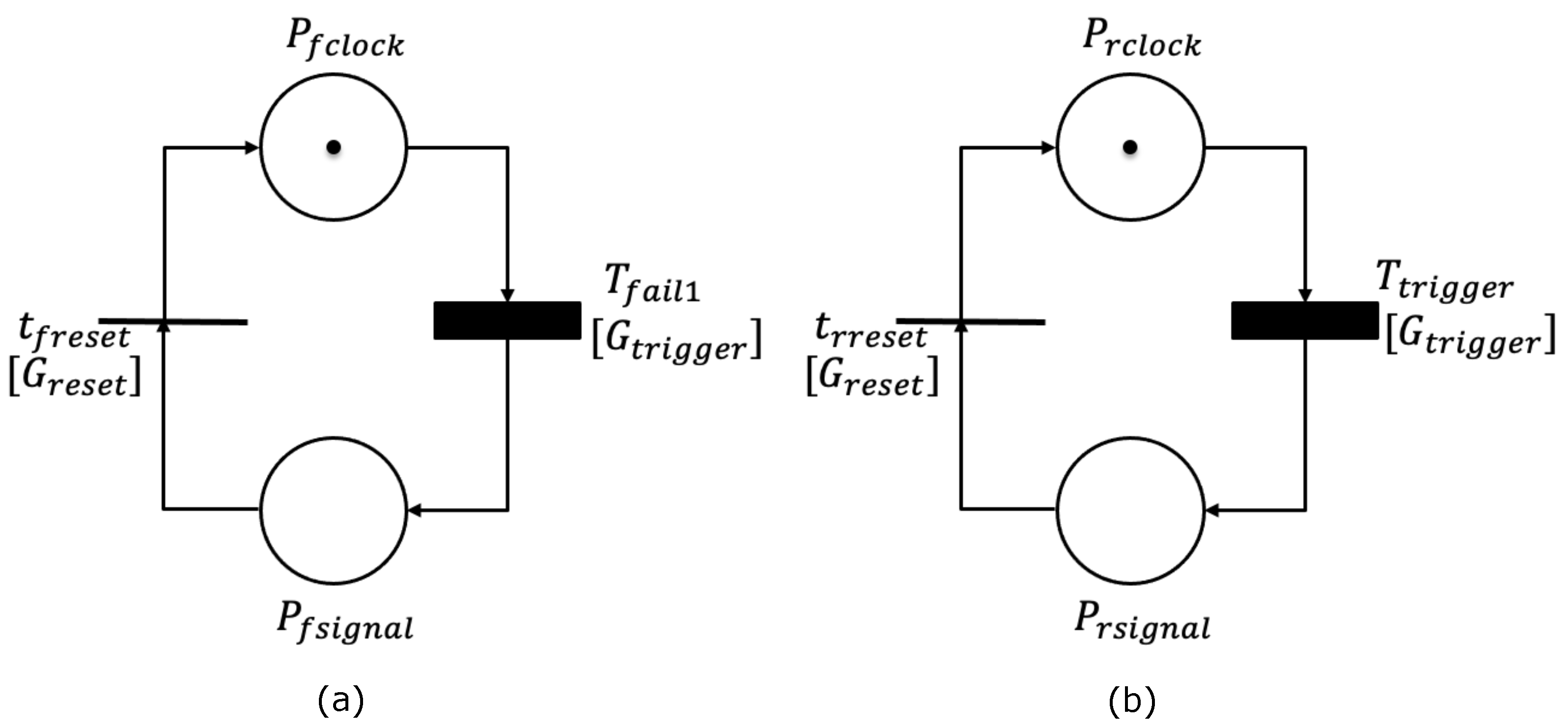
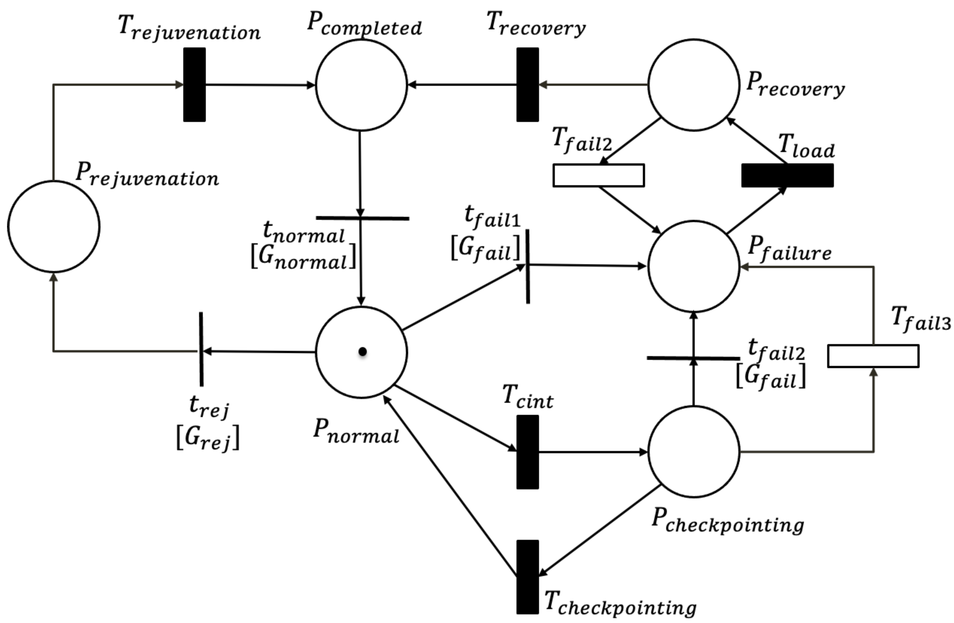
On the basis of the above assumptions, the dynamics of the system are described by a composite SRN as in Figure 1 and Figure 2. Concretely, the composite SRN contains three submodels: clock model for system aging (Figure 1a), clock model for software rejuvenation (Figure 1b), and SRN model for system behavior (Figure 2). In these SRNs, transitions are divided into three types: (i) immediate (IMM) transition (represented by a thin black bar), which means the zero firing time transition; (ii) exponential (EXP) transition (represented by a white rectangle), which refers to the exponentially distributed firing time transition; and (iii) general (GEN) transition (represented by a thick black bar), which is generally distributed firing time transition. The places are defined as follows:

• $P_{fclock}$: software aging accumulates as time passes.
• $P_{fsignal}$: it is time for an aging-related system failure to occur.
• $P_{rclock}$: time is accumulated to trigger a rejuvenation.
• $P_{rsignal}$: a rejuvenation point was reached.
• $P_{normal}$: the system waits for checkpointing and rejuvenation in the normal execution process.
• $P_{checkpointing}$: the system is under checkpointing.
• $P_{rejuvenation}$: the system is under rejuvenation.
• $P_{failure}$: the system fails due to either aging-related bugs or human-error factors, and checkpointed data are loaded for rollback recovery.
• $P_{recovery}$: rollback recovery is executed to recover the failed system.
• $P_{completed}$: the system becomes as good as new after the completion of either rejuvenation or rollback recovery.

On the other hand, transitions $T_{cint}$, $T_{trigger}$, and $T_{fail1}$ correspond to the trigger intervals of checkpointing and rejuvenation, and system lifetime, respectively. Transitions $T_{checkpointing}$, $T_{rejuvenation}$, $T_{load}$, and $T_{recovery}$ separately represent the operations of checkpointing, rejuvenation, loading of checkpointed data, and rollback recovery. Transitions $T_{fail2}$ and $T_{fail3}$ are both EXP transitions, representing failures caused by incorrect operations by the operators. Once IMM transition $t_{rej}$ fires with satisfied guard function $G_{rej}$, the system is immediately rejuvenated. If a token appears in place $P_{fsignal}$, either transition $t_{fail1}$ or transition $t_{fail2}$ fires due to the exhausted lifetime. Transitions $t_{freset}$ and $t_{rreset}$ represent the reset of the clocks, and $t_{normal}$ means that the system becomes normal again at the same time as when clock reset. The details of guard functions are shown in

Table 1. Guard functions.

Guard	Guard Function
$G_{normal}$	#$\left(P_{fclock}\right)=1$ && #$\left(P_{rclock}\right)=1$
$G_{fail}$	#$\left(P_{fsignal}\right)=1$
$G_{rej}$	#$\left(P_{rsignal}\right)=1$ && #$\left(P_{fsignal}\right)=0$
$G_{trigger}$	#$\left(P_{normal}\right)=1$ && #$\left(P_{checkpointing}\right)=1$
$G_{reset}$	#$\left(P_{completed}\right)=1$

.

2.3. Reachability Graph

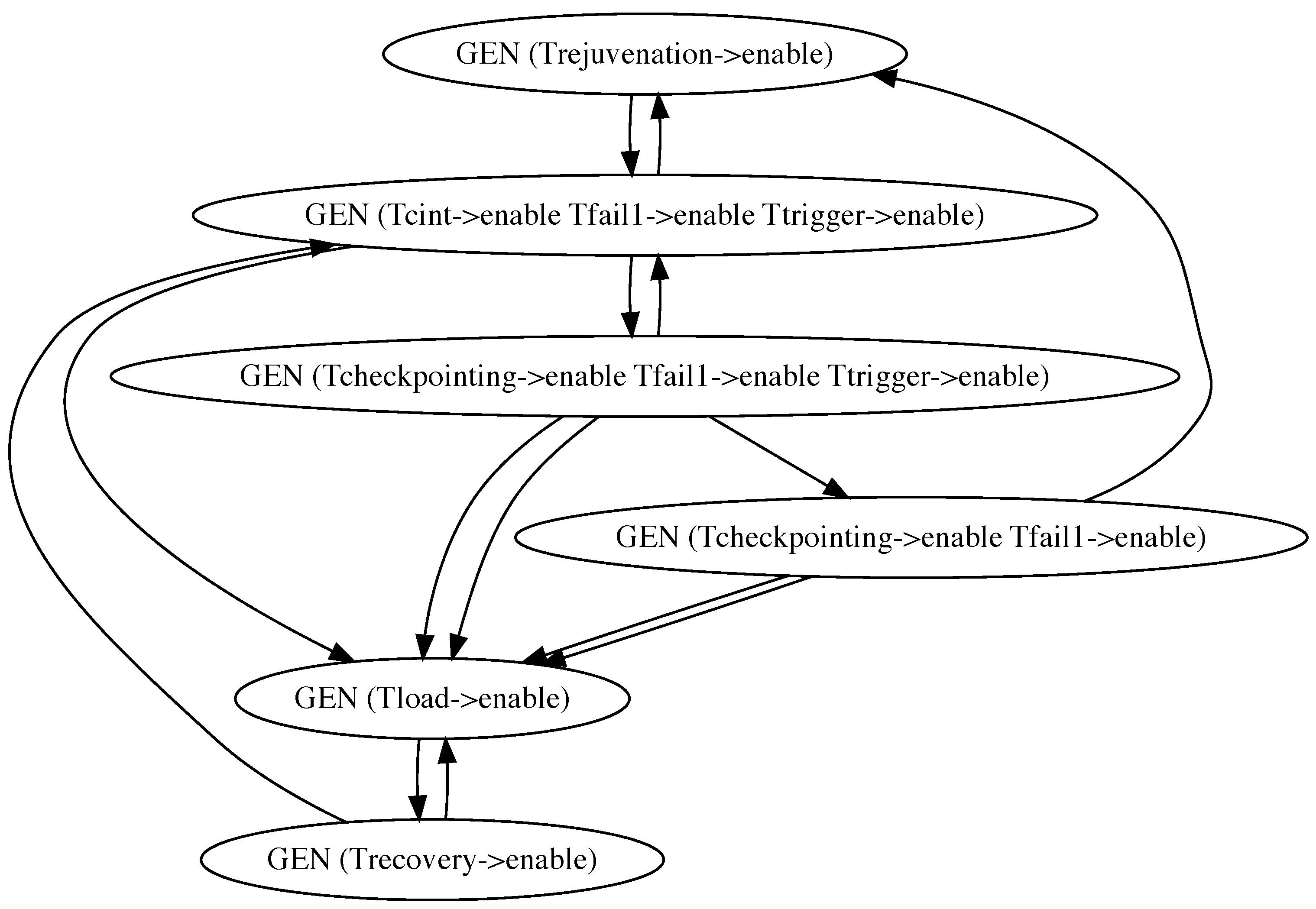
A Petri net’s reachability graph is also a directed graph composed of nodes and edges, each of which representing a reachable marking and a transition between two reachable markings, respectively. According to analysis of the composite SRN described in Section 2.2, a reachability graph, starting with the initial marking $\{P_{normal}:1,P_{fclock}:1,P_{rclock}:1\}$ (here no token places are not shown for brevity), is generated and depicted as in Figure 3. The description of nodes in the graph are summarized in

Table 2. Nodes in reachability graph.

Node	Description
GEN ($T_{cint}$ → enable $T_{fail1}$ → enable $T_{trigger}$ → enable)	Initial marking representing the normal execution state
GEN ($T_{checkpointing}$ → enable $T_{fail1}$ → enable $T_{trigger}$ → enable)	Marking representing checkpointing-execution state with disabled rejuvenation
GEN ($T_{checkpointing}$ → enable $T_{fail1}$ → enable)	Marking representing checkpointing-execution state with enabled rejuvenation
GEN ($T_{load}$ → enable)	Marking representing system-failure state
GEN ($T_{recovery}$ → enable)	Marking representing rollback-recovery state
GEN ($T_{rejuvenation}$ → enable)	Marking representing rejuvenation-execution state

. For example, node GEN ($T_{cint}$→ enable $T_{fail1}$→ enable $T_{trigger}$→ enable) is the initial marking and represents the normal execution state of the system in which all transitions $T_{cint}$, $T_{fail1}$, and $T_{trigger}$ are enable. Both nodes GEN ($T_{checkpointing}$→ enable $T_{fail1}$→ enable $T_{trigger}$→ enable) and GEN ($T_{checkpointing}$→ enable $T_{fail1}$→ enable) correspond to the checkpointing execution states, and the difference between them is whether a rejuvenation point was reached. Node GEN ($T_{load}$→ enable) means that the system failed, and the loading of checkpointed data is being executed. This graph shows that there exist two edges from either node GEN ($T_{checkpointing}$→ enable $T_{fail1}$→ enable $T_{trigger}$→ enable) or node GEN ($T_{checkpointing}$→ enable $T_{fail1}$→ enable) to node GEN ($T_{load}$→ enable). This is explained by the fact that, during checkpointing, the system may fail due to aging-rated bugs or human-error factors, that is, among two edges, one represents the GEN transition $T_{fail1}$ and another corresponds to the EXP transition $T_{fail3}$.

2.4. Non-Markovian State-Transition Diagram

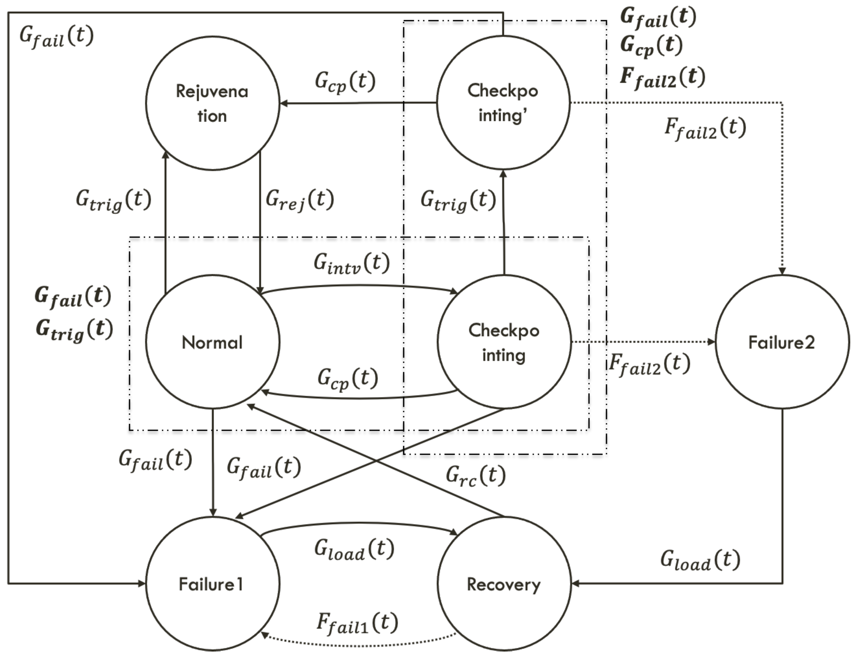
From the reachability graph in Section 2.3, a non-Markovian state-transition diagram was derived as shown in Figure 4. This model consisted of seven states: $Normal$, $Checkpointing$, $Checkpointin{g}^{\prime }$, $Rejuvenation$, $Failure1$, $Recovery$, and $Failure2$. State $Normal$ is the initial state and represents that the system is in the normal execution process in the main memory and waits for the checkpointing and rejuvenation. Once a checkpoint is reached prior to the rejuvenation point, the system state becomes $Checkpointing$, in which data on the main memory are saved in secondary storage. Since the checkpointing operation does not reset the clock of the rejuvenation trigger, a rejuvenation point may be reached during checkpointing. In such a case, the system enters state $Checkpointin{g}^{\prime }$, which represents the checkpoint execution with enabled rejuvenation. After the completion of checkpointing, the system transitions from state $Checkpointin{g}^{\prime }$ to state $Rejuvenation$. If a rejuvenation point is reached prior to the checkpoint, the system immediately executes rejuvenation and enters state $Rejuvenation$ from state $Normal$. As mentioned in Section 2.1, system failure may occur due to aging-related bugs and human-error factors. Thus, two failure states, $Failure1$ and $Failure2$, were defined to distinguish two kinds of system failures. When the system fails, a series of recovery operations, including checkpointed data loading and the rollback recovery, are conducted to recover the system from failure. Lastly, the system becomes $Normal$ again from state $Recovery$. Of course, the system may fail before both checkpointing and rejuvenation. The details of state notation are given in

Table 3. State notation in non-Markovian state-transition diagram.

State	Description
Normal	Normal execution process in the main memory
Checkpointing	Checkpointing execution with a disabled rejuvenation
Checkpointing’	Checkpointing execution with an enabled rejuvenation
Failure1	Aging-related system failure
Failure2	Human-error-related system failure
Recovery	Rollback recovery to recover from system failure
Rejuvenation	Software-rejuvenation execution to refresh system’s internal states

.

Table 4. Cumulative distribution functions (CDFs) of transitions in state-transition diagram.

CDF	Description	Type
$G_{intv}\left(t\right)$	CDF of checkpoint interval.	GEN
$G_{fail}\left(t\right)$	CDF of time for an aging-related failure to occur.	GEN
$G_{cp}\left(t\right)$	CDF of time needed for checkpointing.	GEN
$G_{load}\left(t\right)$	CDF of loading time of checkpointed data.	GEN
$G_{rc}\left(t\right)$	CDF of time needed for rollback recovery.	GEN
$G_{trig}\left(t\right)$	CDF of time required to trigger a rejuvenation.	GEN
$G_{rej}\left(t\right)$	CDF of rejuvenation overhead.	GEN
$F_{fail1}\left(t\right)$	CDF of time for failure to occur during rollback recovery.	EXP
$F_{fail2}\left(t\right)$	CDF of time for a human-error-related failure to occur during checkpointing execution.	EXP

summarizes the cumulative distribution functions (CDFs) of the corresponding transitions in the state-transition diagram. In this table, GEN represents general distribution, and EXP means exponential distribution. The reasons for making such assumptions of probability distributions can be found in [20]. The checkpoint interval was assumed to follow general distribution $G_{intv}\left(t\right)$, and the CDF of the time needed for checkpointing is given by $G_{cp}\left(t\right)$. The time for an aging-related failure to occur follows a general distribution $G_{fail}\left(t\right)$ with increasing failure rate (IFR), while the time distributions for failures occurring during both rollback recovery and checkpointing due to incorrect operations by operators are given by $F_{fail1}\left(t\right)$ and $F_{fail2}$ with constant failure rates (CFRs) ${\lambda }_{fail1}$ and ${\lambda }_{fail2}$, respectively. Similarly, the rejuvenation-trigger interval distribution is described by $G_{trig}\left(t\right)$, and its relevant overhead distribution is represented by $G_{rej}\left(t\right)$. The probability distribution of loading time of checkpointed data and the time needed for rollback recovery are given by $G_{load}\left(t\right)$ and $G_{rc}\left(t\right)$, respectively.

Figure 4 shows states $Normal$ and $Checkpointing$, highlighted by a dashed rectangle with $G_{fail}\left(t\right)$ and $G_{trig}\left(t\right)$, indicating that these GEN transitions regarding $G_{fail}\left(t\right)$ and $G_{trig}\left(t\right)$ are enabled and could fire under either the $Normal$ or the $Checkpointing$ state. In the same way, the dashed rectangle for $Checkpointing$ and $Checkpointin{g}^{\prime }$ means the possible firings of GEN and EXP transitions regarding $G_{fail}\left(t\right)$, $G_{cp}\left(t\right)$, and $F_{fail2}\left(t\right)$. This implies that the non-Markovian state-transition diagram under consideration is neither the SMP nor the MRGP, resulting in difficult numerical analysis. To cope with this issue, in this paper we consider the PH expansion approach [22], which proved to be efficient for solving such kind of non-Markovian state-transition models [19,20,26].

3. System Availability Analysis

This section first introduces the well-known continuous PH distribution [22] and then derives the underlying approximate CTMC for the non-Markovian state-transition diagram in Figure 4 via PH expansion approach, of which the essential idea is to replace general distribution with its corresponding PH distribution at a high accuracy level. Lastly, the stationary solution for the model in Figure 4 through CTMC analysis is presented. The measure of interest is steady-state system availability, which is defined as the probability that the system is operational in the steady state.

3.1. Continuous PH Distribution

Continuous PH distribution is defined as the probability distribution of absorbing time in a finite CTMC with absorbing states, and it is widely applied in various fields, such as reliability assessment [26], queueing systems [27], and random telegraph noise analysis [28]. Without loss of generality, we define $\mathit{Q}$ as an infinitesimal generator matrix of a CTMC that has m transient states and one absorbing state, and then partition $\mathit{Q}$ into four parts as below:

$$\begin{array}{c}\hfill \mathit{Q}=\left(\begin{array}{cc}\mathit{T}& \mathit{\xi }\\ \mathbf{0}& 0\end{array}\right).\end{array}$$

(1)

In the above, $\mathit{T}$ and $\mathit{\xi }$ represent transition rates among transient states and exit rates from transient states to the absorbing state, respectively. Defining $\mathit{\alpha }$ as an initial probability vector over the transient states, we have the CDF and probability density function (PDF) for the continuous PH distribution:

$$\begin{array}{c}\hfill F_{PH}\left(t\right)=1-\mathit{\alpha }exp\left(\mathit{T}t\right)\mathbf{1},f_{PH}\left(t\right)=\mathit{\alpha }{exp}^{\mathit{T}t}\mathit{\xi },\end{array}$$

(2)

where $\mathbf{1}$ is a column vector of ones. Exit vector $\mathit{\xi }$ is given by $\mathit{\xi }=-\mathit{T}\mathbf{1}$. Transient states are called phases in general.

Continuous PH distribution can be categorized into several subclasses according to the structure of $\mathit{T}$ [29]. When phase transition is acyclic, the corresponding PH distribution is called acyclic PH distribution (APH). The APH is the widest class among mathematically tractable PH distributions, and it can be converted into the canonical form (CF), which is the minimal representation of APH with the smallest number of free parameters [30]. The APH and its CF are important from the viewpoint of practical applications because it covers some well-known probability distributions, such as exponential distribution, Erlang distribution, and their mixtures. In particular, canonical form 1 (CF1) is usually considered and defined by

$$\begin{array}{cc}\hfill \mathit{\alpha }& =\left(\begin{array}{cccc}{\alpha }_1& {\alpha }_2& \cdots & {\alpha }_m\end{array}\right),\hfill \end{array}$$

(3)

$$\begin{array}{cc}\hfill \mathit{T}& =\left(\begin{array}{ccccc}-{\beta }_1& {\beta }_1& & & \mathit{O}\\ & -{\beta }_2& {\beta }_2& & \\ & & \ddots & \ddots & \\ & & & -{\beta }_{m-1}& {\beta }_{m-1}\\ \mathit{O}& & & & -{\beta }_m\end{array}\right),\hfill \end{array}$$

(4)

$$\begin{array}{cc}\hfill \mathit{\xi }& =\left(\begin{array}{c}0\\ 0\\ ⋮\\ 0\\ {\beta }_m\end{array}\right),\hfill \end{array}$$

(5)

where ${\alpha }_i\ge 0$, ${\sum }_i{\alpha }_i=1$ and $0<{\beta }_1\le \cdots \le {\beta }_m$ for m phases.

In this paper, continuous PH distribution was applied to approximate all general distributions in the non-Markovian state-transition diagram, that is, to determine PH distribution with parameters $(\mathit{\alpha },\mathit{T},\mathit{\xi })$, which can fit the target distribution well by means of maximum likelihood estimation (MLE) approach [22].

3.2. PH-Expanded CTMC

According to the definition of PH distribution in Section 3.1, we define the general distributions in Table 4 by PH distributions with appropriate phases as follows:

$$\begin{array}{cc}\hfill & F_{intv}^{PH}\left(t\right)=1-{\mathit{\alpha }}_{intv}exp\left({\mathit{T}}_{intv}t\right){\mathbf{1}}_{intv},f_{intv}^{PH}\left(t\right)={\mathit{\alpha }}_{intv}exp\left({\mathit{T}}_{intv}t\right){\mathit{\xi }}_{intv},\hfill \end{array}$$

(6)

$$\begin{array}{cc}\hfill & F_{fail}^{PH}\left(t\right)=1-{\mathit{\alpha }}_{fail}exp\left({\mathit{T}}_{fail}t\right){\mathbf{1}}_{fail},f_{fail}^{PH}\left(t\right)={\mathit{\alpha }}_{fail}exp\left({\mathit{T}}_{fail}t\right){\mathit{\xi }}_{fail},\hfill \end{array}$$

(7)

$$\begin{array}{cc}\hfill & F_{cp}^{PH}\left(t\right)=1-{\mathit{\alpha }}_{cp}exp\left({\mathit{T}}_{cp}t\right){\mathbf{1}}_{cp},f_{cp}^{PH}\left(t\right)={\mathit{\alpha }}_{cp}exp\left({\mathit{T}}_{cp}t\right){\mathit{\xi }}_{cp},\hfill \end{array}$$

(8)

$$\begin{array}{cc}\hfill & F_{load}^{PH}\left(t\right)=1-{\mathit{\alpha }}_{load}exp\left({\mathit{T}}_{load}t\right){\mathbf{1}}_{load},f_{load}^{PH}\left(t\right)={\mathit{\alpha }}_{load}exp\left({\mathit{T}}_{load}t\right){\mathit{\xi }}_{load},\hfill \end{array}$$

(9)

$$\begin{array}{cc}\hfill & F_{rc}^{PH}\left(t\right)=1-{\mathit{\alpha }}_{rc}exp\left({\mathit{T}}_{rc}t\right){\mathbf{1}}_{rc},f_{rc}^{PH}\left(t\right)={\mathit{\alpha }}_{rc}exp\left({\mathit{T}}_{rc}t\right){\mathit{\xi }}_{rc},\hfill \end{array}$$

(10)

$$\begin{array}{cc}\hfill & F_{trig}^{PH}\left(t\right)=1-{\mathit{\alpha }}_{trig}exp\left({\mathit{T}}_{trig}t\right){\mathbf{1}}_{trig},f_{trig}^{PH}\left(t\right)={\mathit{\alpha }}_{trig}exp\left({\mathit{T}}_{trig}t\right){\mathit{\xi }}_{trig},\hfill \end{array}$$

(11)

$$\begin{array}{cc}\hfill & F_{rej}^{PH}\left(t\right)=1-{\mathit{\alpha }}_{rej}exp\left({\mathit{T}}_{rej}t\right){\mathbf{1}}_{rej},f_{rej}^{PH}\left(t\right)={\mathit{\alpha }}_{rej}exp\left({\mathit{T}}_{rej}t\right){\mathit{\xi }}_{rej}.\hfill \end{array}$$

(12)

Here, PH parameters $({\mathit{\alpha }}_x,{\mathit{T}}_x,{\mathit{\xi }}_x)$, $x\in \{intv$, $fail$, $cp$, $load$, $rc$, $trig$, $rej\}$ were estimated on the basis of MLE using an expectation–maximization (EM) algorithm [22,31]. Using the above-estimated PH distributions to replace general distributions, the non-Markovian transition diagram was expanded into an approximate CTMC, alternatively called PH-expanded CTMC, of which the infinitesimal generator matrix is given by

$$\begin{array}{c}\hfill \mathit{Q}=\left(\begin{array}{ccccccc}{\mathit{T}}_{intv}\oplus {\mathit{T}}_{fail}\oplus {\mathit{T}}_{trig}& \left({\mathit{\xi }}_{intv}{\mathit{\alpha }}_{cp}\right)\otimes \mathit{I}\otimes \mathit{I}& & ({\mathbf{1}}_{intv}\otimes {\mathbf{1}}_{fail}\otimes {\mathit{\xi }}_{trig}){\mathit{\alpha }}_{rej}& ({\mathbf{1}}_{intv}\otimes {\mathit{\xi }}_{fail}\otimes {\mathbf{1}}_{trig}){\mathit{\alpha }}_{load}& & \\ \left({\mathit{\xi }}_{cp}{\mathit{\alpha }}_{intv}\right)\otimes \mathit{I}\otimes \mathit{I}& {\mathit{T}}_{cp}\oplus {\mathit{T}}_{fail}\oplus {\mathit{T}}_{trig}\oplus (-{\lambda }_{fail2})& \mathit{I}\otimes \mathit{I}\otimes {\mathit{\xi }}_{trig}& & ({\mathbf{1}}_{cp}\otimes {\mathbf{1}}_{trig}\otimes {\mathit{\xi }}_{fail}){\mathit{\alpha }}_{load}& & ({\mathbf{1}}_{cp}\otimes {\mathbf{1}}_{trig}\otimes {\mathbf{1}}_{fail}\otimes {\lambda }_{fail2}){\mathit{\alpha }}_{load}\\ & & {\mathit{T}}_{fail}\oplus {\mathit{T}}_{cp}\oplus (-{\lambda }_{fail2})& ({\mathbf{1}}_{fail}\otimes {\mathit{\xi }}_{cp}){\mathit{\alpha }}_{rej}& ({\mathit{\xi }}_{fail}\otimes {\mathbf{1}}_{cp}){\mathit{\alpha }}_{load}& & ({\mathbf{1}}_{fail}\otimes {\mathbf{1}}_{cp}\otimes {\lambda }_{fail2}){\mathit{\alpha }}_{load}\\ {\mathit{\xi }}_{rej}({\mathit{\alpha }}_{intv}\otimes {\mathit{\alpha }}_{fail}\otimes {\mathit{\alpha }}_{trig})& & & {\mathit{T}}_{rej}& & & \\ & & & & {\mathit{T}}_{load}& {\mathit{\xi }}_{load}{\mathit{\alpha }}_{rc}& \\ {\mathit{\xi }}_{rc}({\mathit{\alpha }}_{intv}\otimes {\mathit{\alpha }}_{fail}\otimes {\mathit{\alpha }}_{trig})& & & & ({\lambda }_{fail1}\otimes {\mathbf{1}}_{rc}){\mathit{\alpha }}_{load}& (-{\lambda }_{fail1})\oplus {\mathit{T}}_{rc}& \\ & & & & & {\mathit{\xi }}_{load}{\mathit{\alpha }}_{rc}& {\mathit{T}}_{load}\end{array}\right).\end{array}$$

(13)

The infinitesimal generator matrix is derived on the basis of the Kronecker representation [23], and the order of states is {Normal, Checkpointing, Checkpointing’, Rejuvenation, Failure1, Recovery, Failure2}. In Equation (13), ⊕ and ⊗ are the Kronecker product and sum [32], $\mathit{I}$ is an identity matrix, and $1/{\lambda }_{fail1}$ and $1/{\lambda }_{fail2}$ are the mean values of EXP distributions $F_{fail1}\left(t\right)$ and $F_{fail2}\left(t\right)$, say the mean times to failure during rollback recovery and checkpointing, respectively.

Entry $({\mathit{\xi }}_{intv}{\mathit{\alpha }}_{cp}\otimes \mathit{I}\otimes \mathit{I})$ shows that the clock of the rejuvenation trigger is not reset and continuously accumulates, even when the system executes the checkpointing. Since the checkpointing operation just saves the current data and does not refresh system aging, entry $\left({\mathit{\xi }}_{cp}{\mathit{\alpha }}_{intv}\right)\otimes \mathit{I}\otimes \mathit{I}$ indicates that only the clock of checkpointing trigger is reset. When a rejuvenation point is reached while the system is under checkpointing, rejuvenation waits until checkpointing is completed; in such a case, the system transits from $Checkpointing$ to $Checkpointin{g}^{\prime }$ with entry $\mathit{I}\otimes \mathit{I}\otimes {\mathit{\xi }}_{trig}$. Entries $({\mathbf{1}}_{intv}\otimes {\mathit{\xi }}_{fail}{\mathbf{1}}_{trig}){\mathit{\alpha }}_{load}$, $({\mathbf{1}}_{cp}\otimes {\mathbf{1}}_{trig}\otimes {\mathit{\xi }}_{fail}){\mathit{\alpha }}_{load}$, and $({\mathit{\xi }}_{fail}\otimes {\mathbf{1}}_{cp}){\mathit{\alpha }}_{load}$ indicate aging-related failures in both normal and checkpointing states, while entries $({\mathbf{1}}_{cp}\otimes {\mathbf{1}}_{trig}\otimes {\mathbf{1}}_{fail}\otimes {\lambda }_{fail2}){\mathit{\alpha }}_{load}$ and $({\mathbf{1}}_{fail}\otimes {\mathbf{1}}_{cp}\otimes {\lambda }_{fail2}){\mathit{\alpha }}_{load}$ represent human-error-related failures during checkpointing. In addition, the system is regarded to be as good as new after either rollback recovery or rejuvenation, so the corresponding transitions are represented by entries ${\mathit{\xi }}_{rej}({\mathit{\alpha }}_{intv}\otimes {\mathit{\alpha }}_{fail}\otimes {\mathit{\alpha }}_{trig})$, and ${\mathit{\xi }}_{rc}({\mathit{\alpha }}_{intv}\otimes {\mathit{\alpha }}_{fail}\otimes {\mathit{\alpha }}_{trig})$, where $({\mathit{\alpha }}_{intv}\otimes {\mathit{\alpha }}_{fail}\otimes {\mathit{\alpha }}_{trig})$ implies that the clocks of checkpointing trigger, system aging, and rejuvenation trigger are refreshed at the same time.

3.3. Steady-State System Availability

Steady-state system availability gives the probability that the system is operational in the steady state, so that it provides a significant insight into the long-term performance of a repairable system. Let $A_{ss}$ define the steady-state system availability. Then, we can obtain it by

$$\begin{array}{c}\hfill A_{ss}={\mathit{\pi }}_{ss}\mathit{r},\end{array}$$

(14)

where ${\mathit{\pi }}_{ss}$ is the steady-state probability vector of the PH-expanded CTMC, $\mathit{Q}$, and can be computed by solving the following linear equation [33]:

$$\begin{array}{c}\hfill {\mathit{\pi }}_{ss}\mathit{Q}=\mathbf{1},{\mathit{\pi }}_{ss}\mathbf{1}=1,\end{array}$$

(15)

and $\mathit{r}$ is the reward (column) vector of the PH-expanded CTMC and given by

$$\begin{array}{cc}\hfill \mathit{r}& =\left(\begin{array}{c}1\otimes {\mathbf{1}}_{intv}\otimes {\mathbf{1}}_{fail}\otimes {\mathbf{1}}_{trig}\\ 0\otimes {\mathbf{1}}_{cp}\otimes {\mathbf{1}}_{fail}\otimes {\mathbf{1}}_{trig}\\ 0\otimes {\mathbf{1}}_{fail}\otimes {\mathbf{1}}_{cp}\\ 0\otimes {\mathbf{1}}_{rej}\\ 0\otimes {\mathbf{1}}_{load}\\ 0\otimes {\mathbf{1}}_{rc}\\ 0\otimes {\mathbf{1}}_{load}\end{array}\right).\hfill \end{array}$$

(16)

It is clear that the system is only available in the normal execution process state. In this paper, one problem of interest is to determine optimal software-rejuvenation timing that maximizes steady-state system availability.

4. Numerical Illustration

This section is devoted to the numerical illustration of the presented model in Figure 4 by means of phase expansion. Model parameters are summarized in

Table 5. Model parameters.

CDF	Distribution	Mean (h)	CV
$G_{intv}\left(t\right)$	Lognormal	1–10	0.2
$G_{fail}\left(t\right)$	Weilbull	10	0.5
$G_{cp}\left(t\right)$	Lognormal	0.05	0.2
$G_{load}\left(t\right)$	Lognormal	0.5	0.2
$G_{rc}\left(t\right)$	Lognormal	0.5	0.2
$G_{trig}\left(t\right)$	Lognormal	5–35	0.1
$G_{rej}\left(t\right)$	Lognormal	0.5	0.2
$F_{fail1}\left(t\right)$	Exponential	16.67	1
$F_{fail2}\left(t\right)$	Exponential	1.5	1

, where all values are given according to the related literature [13,20,34]. All general distributions were accurately approximated by PH distributions with appropriate phases, that is, 100 phases for $G_{intv}\left(t\right)$, $G_{cp}\left(t\right)$, $G_{load}\left(t\right)$, $G_{rc}\left(t\right)$, $G_{trig}\left(t\right)$, and $G_{rej}\left(t\right)$ and 10 phases for $G_{fail}\left(t\right)$ (see [20] for more details); eventually, we obtained a large approximate CTMC consisting of 201,400 PH-expanded states. Similar to [20], in order to evaluate the effects of the checkpoint interval and the rejuvenation-trigger interval on system availability, the mean checkpoint interval (MCI) was varied from 1 to 10 h, and the mean rejuvenation-trigger interval (MRTI) was changed from 5 to 35 h. In addition, human-error-related system failures both were and were not considered, aiming at quantifying the effects of human-error factors on both system availability and optimal software-rejuvenation timing.

4.1. Steady-State System Availability

Here, we show the steady-state availabilities of a system that may fail due to human error in checkpointing under different cases of MRTI and MCI. The corresponding results are given in

Table 6. Steady-state system availability (with human-error-related system failures). Note: MCI, mean checkpoint interval; MRTI, mean rejuvenation-trigger interval.

MCI (h)	MRTI = 5 h	MRTI = 7 h	MRTI = 10 h	MRTI = 13 h	MRTI = 15 h
1	0.83333	0.84600	0.85168	0.85226	0.85194
2	0.86380	0.87684	0.88245	0.88259	0.88192
3	0.87494	0.88747	0.89309	0.89305	0.89227
4	0.87897	0.89335	0.89846	0.89836	0.89752
5	0.88327	0.89598	0.90182	0.90155	0.90069
6	0.88679	0.89801	0.90404	0.90369	0.90278
7	0.88849	0.90022	0.90531	0.90529	0.90430
8	0.88908	0.90204	0.90635	0.90637	0.90546
9	0.88925	0.90318	0.90740	0.90714	0.90630
10	0.88929	0.90377	0.90838	0.90779	0.90694

, which shows that steady-state system availability increased as the value of MCI increased under each MRTI case. This means that too-frequent checkpointing decreases system availability because the system becomes unavailable during checkpointing. The effect of MRTI on system availability is now examined. For each MCI, steady-state system availability increases at the beginning and subsequently decreases with increasing MRTI, implying that an optimal MRTI might exist for maximizing steady-state system availability.

Moreover, by comparing results in Table 6 and

Table 7. Steady-state system availability (without human-error-related system failures).

MCI (h)	MRTI = 5 h	MRTI = 7 h	MRTI = 10 h	MRTI = 13 h	MRTI = 15 h
1	0.84850	0.86206	0.86796	0.86821	0.86758
2	0.87067	0.88438	0.89024	0.89025	0.88942
3	0.87876	0.89200	0.89788	0.89779	0.89692
4	0.88154	0.89626	0.90174	0.90162	0.90073
5	0.88469	0.89810	0.90415	0.90393	0.90303
6	0.88735	0.89954	0.90576	0.90548	0.90456
7	0.88867	0.90117	0.90666	0.90665	0.90567
8	0.88913	0.90254	0.90741	0.90744	0.90652
9	0.88926	0.90341	0.90818	0.90800	0.90714
10	0.88929	0.90387	0.90892	0.90849	0.90761

, the latter of which gives the steady-state system availability without considering human-error-related system failures, it is reasonable to say that human-error factors significantly decreased system availability, especially in the case where the value of MCI was small. In other words, although frequent checkpointing can save data in a timely manner, it also brings a higher risk of system failure, caused by incorrect operations. Therefore, it is crucial to determine a suitable frequency of executing checkpointing to satisfy target system availability. For example, given a target steady-state system availability of 0.9 and an MRTI of 10 h, an MCI equal to or larger than 5 h is a good choice.

4.2. Optimal Rejuvenation-Trigger Timing

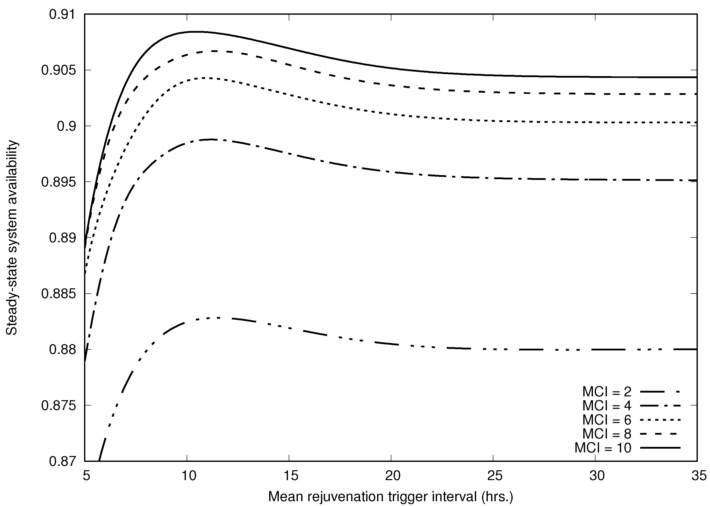
This subsection discusses optimal software-rejuvenation timing maximizing steady-state system availability. Figure 5 illustrates the sensitivity of steady-state system availability with respect to the mean rejuvenation-trigger interval in the cases of $\mathrm{MCI}=2,4,6,8$ and 10. The figure plots unimodal curves of the steady-state system availabilities, which reveals the existence of optimal rejuvenation-trigger timing maximizing steady-state system availability in each case. Specifically, the overhead incurred by frequent rejuvenation (i.e., short MRTI) largely affects system availability. Conversely, downtime due to system failures caused by a less frequent execution of rejuvenation smoothly decreases system availability.

Optimal rejuvenation-trigger timings and their corresponding maximal steady-state system availabilities in all cases are presented in

Table 8. Optimal rejuvenation-trigger timings.

MCI (h)	with Human-Error-Related Failures		without Human-Error-Related Failures
	MRTI (h)	${\mathit{A}}_{\mathit{ss}}$	MRTI (h)	${\mathit{A}}_{\mathit{ss}}$
1	12.3	0.85230	11.6	0.86841
2	11.5	0.88283	11.3	0.89059
3	11.3	0.89339	11.2	0.89819
4	11.2	0.89878	11.2	0.90206
5	11.0	0.90196	11.1	0.90435
6	10.9	0.90428	11.0	0.90603
7	11.3	0.90572	11.3	0.90708
8	11.4	0.90668	11.4	0.90777
9	11.0	0.90753	11.1	0.90838
10	10.5	0.90842	10.7	0.90902

. We present all optimal rejuvenation timings for the system regardless of considering human-error-related system failures. Optimal MRTIs for all cases of MCI were very similar, which means that the optimal rejuvenation-trigger timing is not very sensitive to checkpoint interval. Optimal MRTIs in the case where human-error-related system failures were not considered were slightly smaller than those in the case with human-error-related failure when the value of MCI was small, and vice versa when the MCI had a large value, for example, $\mathrm{MCI}=9,10$.

5. Conclusions

In this paper, we presented a composite stochastic Petri reward net and its resulting non-Markovian availability model for operational software systems where both checkpointing and software rejuvenation are adopted to protect data and to enhance the system availability, and the system may fail due to both the aging problem and human errors during checkpointing. More specifically, the non-Markovian availability model was derived on the basis of a reachability graph that was generated from the original SRNs. In particular, the PH expansion approach was applied to solve the stationary solution of the non-Markovian availability model since the model was not one of the trivial stochastic models such as SMP and MRGP, so that common approaches such as LST and embedded Markov chain techniques do not work. Numerical results showed that human-error factors both decreased steady-state system availability and brought a significant effect on optimal rejuvenation-trigger timing, which means that human-error factors during system modeling should not be overlooked.

The model presented in this paper was based on a macroscopic view, providing a fundamental idea of how to model such a software system that undergoes both checkpointing and software rejuvenation, and in which the system behaves with multiple competitive events. The system’s actual behavior is very complex, and more possible events need to be considered, for example, software environment upgrades and time-scope limitations of used versions of libraries. Although this improvement may vastly increase difficulty in numerical analysis, it is significant to take a microscopic look at system behavior, which will be one of our future directions. This paper only considered both aperiodic checkpointing and software rejuvenation, but to the best of our knowledge, there exist various kinds of checkpointing [35] and rejuvenation techniques [8]. In the future, we aim to extend this work to solve more complicated software systems considering different rejuvenation and checkpointing schemes.

References

- Grottke, M.; Trivedi, K.S. Fighting bugs: Remove, retry, replicate, and rejuvenate. IEEE Comput. 2007, 40, 107–109. [Google Scholar] [CrossRef]
- Dohi, T.; Trivedi, K.S.; Avritzer, A. Handbook of Software Aging and Rejuvenation: Fundamentals, Methods, Applications, and Future Directions; World Scientific: Singapore, 2020. [Google Scholar]
- Huang, Y.; Kintala, C.; Kolettis, N.; Funton, N.D. Software rejuvenation: Analysis, module and applications. In Proceedings of the 25th IEEE International Symposium on Fault Tolerant Computing (FTC’95), Pasadena, CA, USA, 27–30 June 1995; pp. 381–390. [Google Scholar]
- Trivedi, K.S.; Vaidyanathan, K. Software aging and rejuvenation. In Wiley Encyclopedia of Computer Science and Engineering; John Wiley and Sons: Hoboken, NJ, USA, 2007; pp. 1–8. [Google Scholar]
- Alonso, J.; Matias, R.; Vicente, E.; Maria, A.; Trivedi, K.S. A comparative experimental study of software rejuvenation overhead. Perform. Eval. 2013, 70, 231–250. [Google Scholar] [CrossRef]
- Vaidyanathan, K.; Trivedi, K.S. A comprehensive model for software rejuvenation. IEEE Trans. Depend. Secur. Comput. 2005, 2, 124–137. [Google Scholar] [CrossRef]
- Ning, G.; Zhao, J.; Lou, Y.; Alonso, J.; Matias, R.; Trivedi, K.S.; Yin, B.B.; Cai, K.Y. Optimization of two-granularity software rejuvenation policy based on the Markov regenerative process. IEEE Trans. Reliab. 2016, 65, 1630–1646. [Google Scholar] [CrossRef] [Green Version]
- Zheng, J.; Okamura, H.; Li, L.; Dohi, T. A comprehensive evaluation of software rejuvenation policies for transaction systems with Markovian arrivals. IEEE Trans. Reliab. 2017, 66, 1157–1177. [Google Scholar] [CrossRef]
- Dohi, T.; Zheng, J.; Okamura, H.; Trivedi, K.S. Optimal periodic software rejuvenation policies based on interval reliability criteria. Reliab. Eng. Syst. Saf. 2018, 180, 463–475. [Google Scholar] [CrossRef]
- Wang, S.; Liu, J. HARRD: Real-time software rejuvenation decision based on hierarchical analysis under weibull distribution. In Proceedings of the 20th IEEE International Conference on Software Quality, Reliability and Security (QRS’20), Macau, China, 11–14 December 2020; pp. 83–90. [Google Scholar]
- Zhang, Y.; Chakrabarty, K. Fault recovery based on checkpointing for hard real-time embedded systems. In Proceedings of the 18th IEEE Symposium on Defect and Fault Tolerance in VLSI Systems (DFT’03), Boston, MA, USA, 5 November 2003; pp. 320–327. [Google Scholar]
- Fukumoto, S.; Kaio, N.; Osaki, S. Optimal checkpointing policies using the checkpointing density. J. Inf. Process. 1992, 15, 87–92. [Google Scholar]
- Dohi, T.; Osajima, S.; Kaio, N.; Osaki, S. On the effects of checkpoint institution methods for a macroscopic database model. Electron. Commun. Jpn. Part III Fundam. Electron. Sci. 2000, 83, 23–33. [Google Scholar] [CrossRef]
- Ranganathan, A.; Upadhyaya, S.J. Performance evaluation of rollback-recovery techniques in computer programs. IEEE Trans. Reliab. 1993, 42, 220–226. [Google Scholar] [CrossRef]
- Bajunaid, N.; Menascé, D.A. Efficient modeling and optimizing of checkpointing in concurrent component-based software systems. J. Syst. Softw. 2018, 139, 1–13. [Google Scholar] [CrossRef]
- Sigdel, P.; Tzeng, N.F. Coalescing and deduplicating incremental checkpoint files for restore-express multi-level checkpointing. IEEE Trans. Parallel Distrib. Syst. 2018, 29, 2713–2727. [Google Scholar] [CrossRef]
- Okamura, H.; Dohi, T. Comprehensive evaluation of aperiodic checkpointing and rejuvenation schemes in operational software system. J. Syst. Softw. 2010, 83, 1591–1604. [Google Scholar] [CrossRef] [Green Version]
- Levitin, G.; Xing, L.; Luo, L. Joint optimal checkpointing and rejuvenation policy for real-time computing tasks. Reliab. Eng. Syst. Saf. 2019, 182, 63–72. [Google Scholar] [CrossRef]
- Zheng, J.; Okamura, H.; Dohi, T. A phase expansion for non-Markovian availability models with time-based aperiodic rejuvenation and checkpointing. Commun. Stat-Theory Methods 2020, 49, 3712–3729. [Google Scholar] [CrossRef]
- Zheng, J.; Okamura, H.; Dohi, T. Optimal rejuvenation policies for non-Markovian availability models with aperiodic checkpointing. IEICE Trans. Inf. Syst. 2020, E103-D, 2133–2142. [Google Scholar] [CrossRef]
- Bolch, G.; Greiner, S.; De Meer, H.; Trivedi, K.S. Queueing Networks and Markov Chains: Modeling and Performance Evaluation with Computer Science Applications, 2nd ed.; John Wiley and Sons: New York, NY, USA, 2006. [Google Scholar]
- Okamura, H.; Dohi, T. Fitting phase-type distributions and Markovian arrival processes: Algorithms and tools. In Principles of Performance and Reliability Modeling and Evaluation; Lance, F., Antonio, P., Eds.; Springer: Berlin/Heidelberg, Germany, 2016; pp. 49–75. [Google Scholar]
- Trivedi, K.S.; Bobbio, A. Reliability and Availability Engineering: Modeling, Analysis, and Applications; Cambridge University Press: Cambridge, UK, 2017. [Google Scholar]
- Brown, A. An Overview of Human Error. CS294-4 ROC Semin. 1990, 54. Available online: http://roc.cs.berkeley.edu/294fall01/slides/human-error.pdf (accessed on 10 December 2020).
- Yanagihara, M.; Odagiri, M.; Osaki, S.; Kaio, N. Optimal checkpointing procedures taking into account system failure caused by checkpointing. Electron. Commun. Jpn. Part III Fundam. Electron. Sci. 1995, 78, 69–79. [Google Scholar] [CrossRef]
- Zheng, J.; Okamura, H.; Dohi, T. A transient interval reliability analysis for software rejuvenation models with phase expansion. Softw. Qual. J. 2020, 28, 173–194. [Google Scholar] [CrossRef]
- Yang, X.; Alfa, A.S. A class of multi-server queueing system with server failures. Comput. Ind. Eng. 2009, 56, 33–43. [Google Scholar] [CrossRef]
- Ruiz-Castro, J.E.; Acal, C.; Aguilera, A.M.; Roldán, J.B. A complex model via phase-type distributions to study random telegraph noise in resistive memories. Mathematics 2021, 9, 390. [Google Scholar] [CrossRef]
- Kemper, P.; Müller, D.; Thümmler, A. Combining response surface methodology with numerical methods for optimization of Markovian models. IEEE Trans. Depend. Secur. Comput. 2006, 3, 259–269. [Google Scholar] [CrossRef]
- Cumani, A. On the canonical representation of homogeneous Markov processes modelling failure-time distributions. Microelectron. Reliab. 1982, 22, 583–602. [Google Scholar] [CrossRef]
- Okamura, H.; Dohi, T.; Trivedi, K.S. Improvement of EM algorithm for phase-type distributions with grouped and truncated data. Appl. Stoch. Model. Bus. Ind. 2013, 29, 141–156. [Google Scholar] [CrossRef]
- Dayar, T. Analyzing Markov Chains Using Kronecker Products: Theory and Applications; Springer Science and Business Media: New York, NY, USA, 2012. [Google Scholar]
- Trivedi, K.S. Probability and Statistics with Reliability, Queuing, and Computer Science Applications, 2nd ed.; John Wiley and Sons: Hoboken, NJ, USA, 2001. [Google Scholar]
- Leung, C.H.C.; Currie, E. The effect of failures on the performance of long-duration database transactions. Comput. J. 1995, 38, 471–478. [Google Scholar] [CrossRef] [Green Version]
- Tantawi, A.N.; Ruschitzka, M. Performance analysis of checkpointing strategies. ACM Trans. Comput. Syst. 1984, 2, 123–144. [Google Scholar] [CrossRef]
Figure 1.
Clock models for (a) system aging and (b) software rejuvenation.
Figure 2.
Stochastic (Petri) reward net (SRN) model for system behavior.