Short-Scale Stochastic Solar Energy Models: A Datacenter Use Case


1
Inria, Université Côte d’Azur, 06902 Sophia Antipolis, France
2
Inria, LIRMM, University Montpellier, CNRS, 34095 Montpellier, France
*
Authors to whom correspondence should be addressed.
†
The authors contributed equally to this work.
Mathematics 2020, 8(12), 2127; https://doi.org/10.3390/math8122127
Submission received: 30 October 2020
/
Revised: 23 November 2020
/
Accepted: 24 November 2020
/
Published: 27 November 2020
(This article belongs to the Special Issue Queue and Stochastic Models for Operations Research)
Abstract
:Modeling the amount of solar energy received by a photovoltaic panel is an essential part of green IT research. The specific motivation of this work is the management of the energy consumption of large datacenters. We propose a new stochastic model for the solar irradiance that features minute-scale variations and is therefore suitable for short-term control of performances. Departing from previous models, we use a weather-oriented classification of days obtained from past observations to parameterize the solar source. We demonstrate through extensive simulations, using real workloads, that our model outperforms the existing ones in predicting performance metrics related to energy storage.
1. Introduction
It is now a well-known fact that the energy footprint of information technologies now accounts for a sizeable proportion of global energy consumption, and that the operations of datacenters are responsible for a large fraction of it. As argued in [1], major companies operating huge datacenters are interested in taking advantage of “green” renewable energy resources, both for the sake of saving money and for participating in the emission reductions. Powering datacenters with (at least some) locally produced solar energy is an attractive possibility. On the other hand, it is also well-known that renewable energy resources, such as wind and sunlight, feature large variability, which adds up in the variability of the workload. In these conditions, the management of datacenters involves much flexibility in, e.g., scheduling of jobs and equipment, and pricing of services [2,3,4]. The models allowing one to compute these policies require accurate models of the stochastic solar energy input.
1.1. The Need for Accurate Models of Solar Irradiance
In this paper, we propose a new model for stochastic sources of solar light, and advocate its use when studying the performance, static and dynamic optimization or dimensioning of datacenters.
First, as we shall demonstrate in our experiments, the existing models fail to accurately predict the basic performance metrics for energy storage: battery shortage and energy spillover. We depart from the usual approach by not considering long-duration, multi-day models. Our point of view is that stationarity scarcely occurs, even within one day, and that discussing the transitions from one day to the next is unnecessary.
We base that point of view on the following use case scenario. The datacenter manager (DM) plans the resources (computing units in service, purchase of energy on the market, etc.) one or several days ahead. He/she will use simulations to investigate several scenarios and optimize some criteria. A model is needed for the solar energy input that next day (also for the workload of the datacenter but that is outside the scope of this paper). Like anybody in the world, the DM has access to weather info about the next day. Given the financial stakes, it can be assumed that the DM has the means to buy a precise weather outlook. Datacenter managers also have the means to obtain astronomical and geographical data such as the time of sunrise and sunset every day, and the value of the clear-sky irradiance (see Section 2). In summary, what is needed here is a one-day stochastic model, parametrized by some prediction about the kind of weather available some time ahead.
Second, we believe that a correct way to assess the quality of a solar source model is through a “queuing evaluation”. We mean by this that instead of focusing on the arrival process of energy with methods of the signal processing literature (as we have ourselves done in [5]), it is necessary to evaluate the quality of a source through its performance in a finite queue. We believe this is relevant for several reasons. On the one hand, as already argued, there is no clear stationarity in the processes, so that spectral analysis may not be relevant, or is difficult to interpret. On the other hand, queuing systems (especially with finite capacity) are not linear systems, so that the dependence of their response on the spectrum of a signal is not immediate to see. Finally, many queuing models of datacenter consumption and optimization are being developed in the literature ([1,2,3,6,7,8] to quote just a few): they need a realistic energy source model, and a realistic consumption model. We devote this work to the first element, the second having been taken from real (therefore realistic) traces.
1.2. Related Work
Models of solar irradiance and of the transformation of irradiance into electric current are not new in the literature. As we will argue for shortly, we are not interested in the detailed modeling of transformation and we concentrate on irradiance itself. Models in the literature differ in purpose and the data they use. Some models aim at capturing the accumulated sunlight on the scale of days or weeks, which is relevant for predicting the responses of vegetation. Others consider smaller time scales: days, hours or minutes depending on the application envisioned.
To set the context for this review, we introduce first the relevant vocabulary. The global solar irradiance refers to the amount of solar energy reaching a specific area and is expressed in W/m. It varies over the course of the day and from one day to another; we will therefore denote it as where d stands for “day” and m stands for “minute”. The ideal value of this irradiance occurs when no clouds or obstacle are present: this clear sky irradiance is denoted with . The global solar irradiance is seen as the result of applying a multiplicative “noise” to the clear sky irradiance . This corresponds to the decomposition:
where we have used the notation to refer to the clear sky index which is how the multiplicative noise is known in the literature.
The literature features many models for the (deterministic) clear sky irradiance function , as surveyed by Dave, Halpern and Myers in [9] and by Bird and Hulstrom in [10]. These authors propose themselves a model in [11], which we later refer to as “Bird’s model”, which involves many physical parameters and consequently requires the knowledge or measurements of many quantities. Other models, such as [12], are simpler to use.
The stochastic models which aim at representing the variations of with respect to its ideal value use two different approaches. One direct statistical approach is to consider the function as a time series and characterize its distribution. This is the approach of [13], in which the non-stationary process is classically decomposed as
where is a slowly varying trend, the seasonal (here, daily) component and some ARMA process. We do not believe the stochastic component is likely to have the same characteristics throughout a year, so that some month-dependence is likely to be better. It is also dubious that such a model would spontaneously generate zero values at night, as it should. In addition, the fitting of one ARMA model on real data involves, according to [13], some exploration of the combinations of parameters, and some data-dependent tuning of learning parameters. We have chosen not to try this model in a first approach. The direct generation of is also the topic of Miozzo et al. in [14], who based their model on semi-Markov processes. We shall present this model in Section 2 and compare it with our proposal.
An alternative approach is to use the decomposition (1) and find a model for the random process . There is a body of literature devoted to the characterization of the distribution of at a given time. Examples are Suehrcke and McCormick [15] and Jurado et al. in [16], who argue that this distribution can be seen as a mixture of two normal distributions. As reported by Ghiassi et al. in [17], the time-dependent process is then modeled as a Levy process, but this modeling is dismissed there, as trajectories generated are very different in shape from actual ones. We shall not consider this model further in our study. Statistics on the temporal behavior of the process were obtained by Gu et al. in [18]: they demonstrate that there are several temporal scales in the correlations of this process at the minute level. Despite this global understanding of the phenomenon, no model seems to emerge for generating synthetic traces of it, at the minute level. In [5], we proposed such a model as a semi-Markov process with a finite number of states, to which some random noise is added. Although promising, this approach lacked the dependency on seasons and weather, and also produced trajectories with excessive variations.
Finally, note that the question to decide whether a solar irradiance model is “good” or not is not entirely solved, as discussed in [19]. We consider that the use-case is what decides: a given model may prove accurate in some situations and not in others. We favor validation through the response of a storage system.
As conclusion of this review, we argue that there are still needs for (a) models in the scale of minutes, and (b) convincing validation of the accuracy of these models in scenarios involving datacenters.
Contributions
The main contributions of this paper are:
- A forecast-based solar energy model that captures the small-scale fluctuations that the global irradiance exhibits. As will be shown in the paper, our model can be used to generate trajectories that closely mimic measured data, a feature unseen in state-of-the-art models.
- A practical use case scenario: We simulated a datacenter fed by solar energy through photovoltaic panels, in which the captured solar energy is stored in batteries. Through simulations we show that our energy model achieves the same performance as benchmarks: the distribution of the battery level is reasonably similar. None of the state-of-the-art models that we tested achieved matching results like our model did.
1.3. Organization of the Paper
The rest of the paper is structured as follows. Section 2 presents the problem of modeling the solar energy and its challenges, and reviews some of the models found in the literature. Section 3 introduces our model of a datacenter fed by a dual energy supply, solar energy and grid, and discusses our main assumptions. Section 4 details our methodology to construct an energy source and presents the energy consumers that we will use in the experiments. Section 5 presents the setup of our experiments and the results that we obtained. Section 6 concludes the paper and presents some perspectives.
2. Solar Energy Models
In this section, we present the models we will use for comparisons in the experimental evaluation. We begin with a discussion on the challenges of modeling the clear sky index .
2.1. Challenges
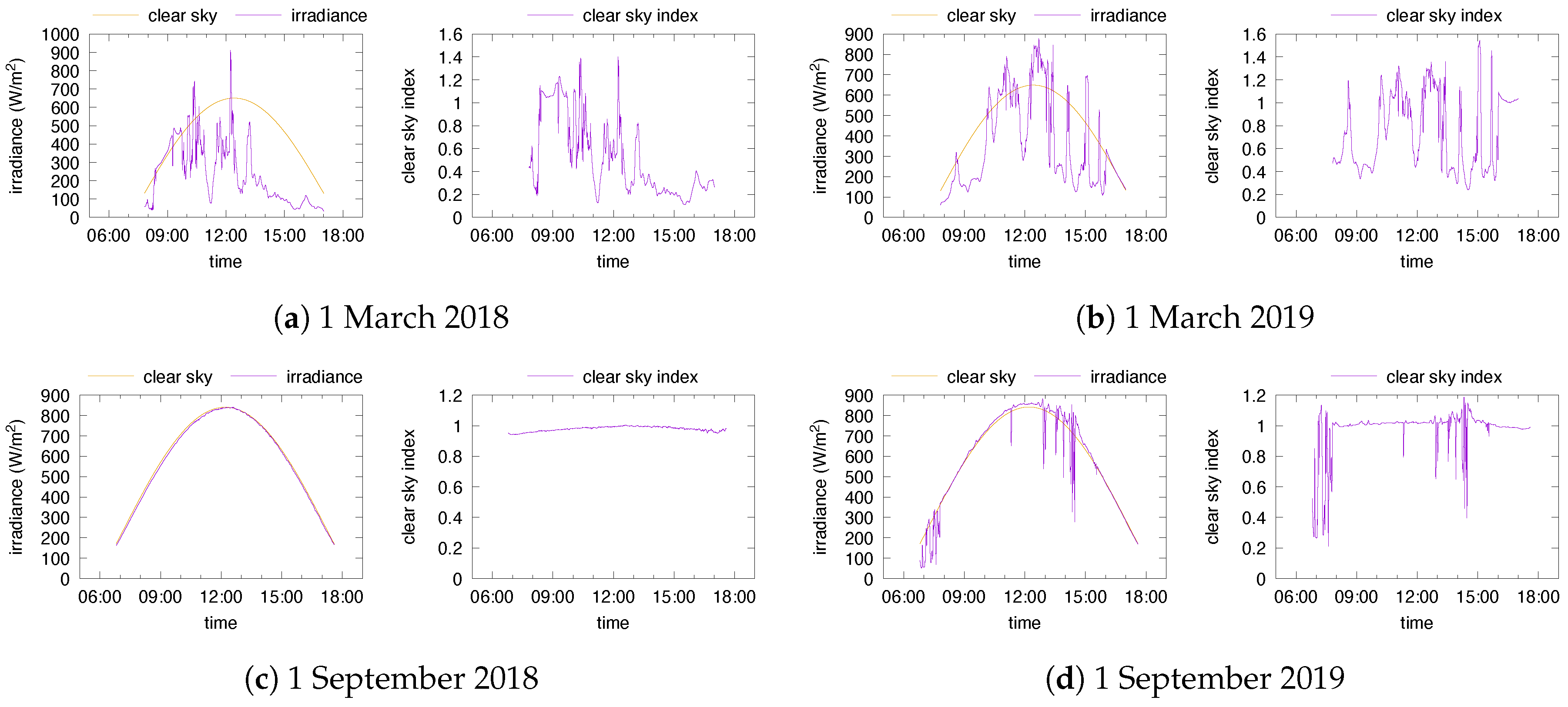
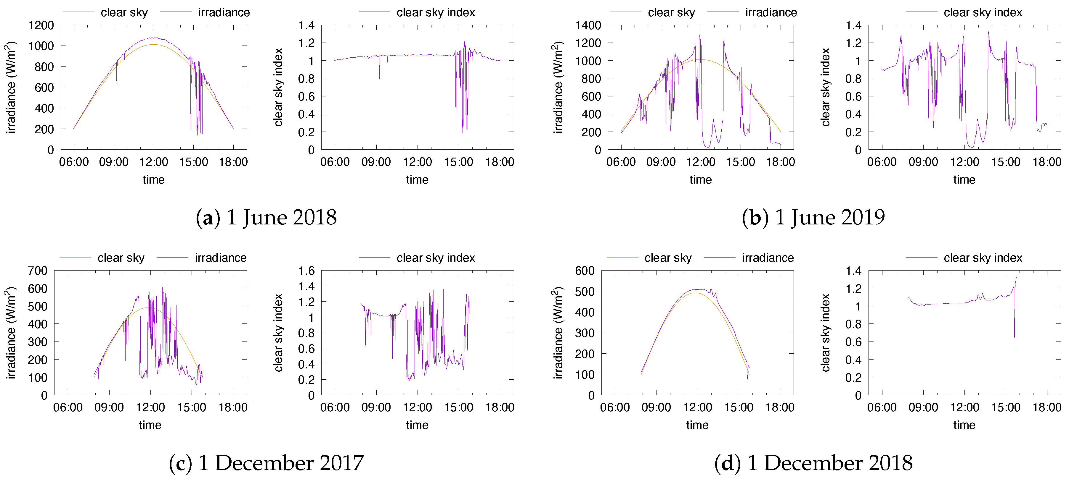
To illustrate the challenges faced in the process of modeling the solar energy, we depict in Figure 1 and Figure 2 the global irradiance on selected days as measured by [20,21] in the cities of Portland (Oregon, US) and Golden (Colorado, US) respectively. Each row of Figure 1 and Figure 2 displays the data relative to a specific day, but one year apart. Each subfigure shows the global and clear sky irradiance on the left and the clear sky index on the right. We can make several observations: First, each day has its own clear sky irradiance curve that depends on astronomical data such as sunset and sunrise, but also on total ozone, surface pressure and ground albedo, to name a few of the impactful factors. Second, very large daily fluctuations can be observed in the global irradiance, even for short intervals, as seen, for instance, in Figure 1d and Figure 2a. Third, none of the data displayed appear to be stationary, not even the clear sky index.
2.2. Models for the Clear Sky Irradiance
As mentioned in Section 1.2, the literature features many models of , with varying degrees of complexity. Whatever the model, it can be assumed that datacenter managers have the financial and technical means to obtain this function at the location of their facility.
It is more difficult for us to do so, so we will rely on the data publicly available that feature the computation of Bird’s model in addition to measurements. In addition, for some of our simulations, we use a simplified sinusoidal model: we assume that the curve of every day d is a pure sine function characterized by two values: the length of the day and the maximal irradiance . Assuming in addition that the maximum is reached at noon, these values are sufficient to define a unique function with equation:
where T is the full day length. The values of and for a given location can be retrieved from, e.g., [22]. If required, the model can be easily modified to account for a sunrise time , a sunset time and a maximum halfway between them.
2.3. Models for the Direct Irradiance
Miozzo et al. in [14] proposed two models for the function . Both models assume that the process is a semi-Markov process.
The simpler model, which we denote as the “daily” (or “day/night”) model in what follows, consists of separating day and night, and modeling the irradiance during the day as a random variate drawn from a month-dependent distribution. In our notation,
where denotes the month to which day d belongs, are twelve independent families of i.i.d. random variables and is an on/off renewal process with values in .
In the second model, which we denote as the “hourly” model in what follows, the irradiance depends on the hour in addition to the month. In our notation,
where , are 12 × 24 independent sequences of i.i.d. random variables. In this model, the semi-Markov process has 24 states; the sojourn time in every state is deterministic and equal to one hour; and transitions are deterministic as well.
In the experiments, we have replaced the (semi-Markov) on/off process of the daily model, with a deterministic day/night alternation based on the astronomical sunrise and sunset times. Since that is readily available information (e.g., [22]), it seems unnecessary to try to guess it statistically.
2.4. Models for the Clear Sky Index
In [12], the function is constructed using an astronomical model, and the function is assumed to be constant throughout the day, with a value that depends on a cloudiness value N through the equation:
The value of N is measured in oktas and lies between 0 (no clouds) and 8 (eight-eighths of the sky covered). The average cloudiness for a given location is commonly measured by weather stations and averaged over one month. In our notation, we then write to reflect this dependence on the current month. References [23,24] provide some (partial) data for Portland, Oregon and Denver, Colorado, for 2001. Since this dataset is incomplete, we have interpolated it for the missing months. The data are displayed in Table 1.
3. Datacenter Model
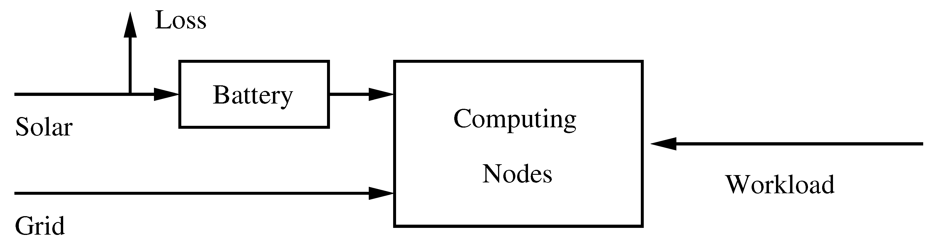
We model the datacenter (DC) with a simple flow and storage model illustrated in Figure 3. The energy supplied to the DC comes from two sources: the solar energy, via photovoltaic panels, and the grid. The solar energy feeds a battery. When the battery is full, the energy is lost. The battery has priority over the grid: if it is not empty, if is used by the energy consumer. If it is empty, the energy is taken from the grid.
The energy consumed by the DC is due to the functioning of computing units, called “nodes” in the remainder. This consumption depends in turn on the number of nodes that are actually busy executing jobs. The number of jobs running in the DC at a given time, which we call the workload, is assumed to be exogenous. In other words, we do not model the complex process of job submitting, queuing, scheduling, abandoning, etc., as observed in [25]. In our experiments, we will use traces of real datacenters from which we extract this number of running jobs at every instant. Those will be described in Section 4.2.
Since our focus is on modeling the solar irradiance process, we did not develop complex models of: (a) transformation of the irradiance into electric current; (b) fine points of datacenter energy consumption: cooling, starting/stopping machines, etc.
For (a) we use a simple linear model, assuming that the electric power coming in the DC is directly proportional to solar irradiance. It is well-known that photovoltaic (PV) panels only capture a proportion of the irradiance and that this proportion depends, in particular, on temperature. Additionally, the current that comes out of the PV suffers losses before it can be used by the DC. Since in our assumption, the proportion is fixed, we will not mention its value explicitly and present all panel surface values in efficient square meters: the surface necessary to produce an electric power equal to the unit irradiance, measured in W/m.
For (b) we use a simple affine model, assuming that nodes have a consumption when idle, and when busy. Accordingly, given that the DC has computing nodes, a workload of is converted into power with the following equation:
Obviously, a precise modeling of these elements is mandatory for building a useful model of a complete datacenter. However, we are not interested in accurate modeling of the datacenter, but only of the irradiance. We make the working assumption that, albeit imprecise, the energy transformation and consumption models we use are sufficiently representative of reality to validate the irradiance model.
4. Methodology
In this section, we discuss the processing of real data that we have performed. In Section 4.1, we present our new solar source model and the way its parameters are learned. In Section 4.2, we describe the workload data and how we used it.
4.1. Forecast-Based Sources
Our driving idea for constructing a solar source is that the curve essentially depends on the type of the day, referring to the sort of weather this day enjoys. Mathematically, we refine the model in (1) into:
The notation refers to the type of the day which defines the weather conditions observed/predicted for that day. We assume where is the set of day types, finite and hopefully not too large. In the experiments of Section 5 we consider models where the number of day types ranges from 2 to 16.
For any , we assume that there is a sequence of distributions , for such that the clear sky index is a random variable following the distribution .
For a given day d of type , it is then possible to characterize the global irradiance using a model for and i.i.d. sequences , drawn from distributions , with:
In order to classify the days in the type set , we start from per-minute irradiance data for two locations, Portland (Oregon, US; see [20]) and Golden (Colorado, US; see [21]) for a 3-year period of time. In addition to the global irradiance, the data [20,21] report predictions of the clear sky irradiance using Bird’s model [11]. We rely on these predictions of to compute the clear sky index according to (5). The subsequent step is to identify which features of days will be used for the classification.
The type of the day can be seen as a description of the weather forecast for that day. In its simplest expression, a day can be seen as “sunny” or “cloudy”, but much more detailed descriptions can be envisaged: hourly conditions may be available/predicted and a finer categorization of the sky condition may be done. When identifying the day type, one can rely on the average value of the clear sky index over the entire day, or on the average values obtained over a number of intervals partitioning the day’s duration. Partitioning the whole duration of the day in fixed intervals throughout the year is not adequate, since the quantity is measured only during daylight time. We will therefore consider that daylight time is split in a number I of equally sized intervals, seen as “phases” of the day, during which the distribution of is assumed to be constant. This refines the model in (6) into:
where m is a minute during daylight time, is the interval number of minutes m in day d and are independent sequences of i.i.d. random variables. We limit the value of I to 12 in our experiments. Consequently, the shortest days in the year in Portland with ∼433 min would have eleven 36-min long intervals and one 37-min long interval. In Golden, with ∼461 min, the shortest days in the year would have seven 38-min long intervals and five 39-min long ones. (Slight variations exist over the years; these figures are those seen in the training and testing data).
To estimate day types, we use the Scikit-learn Python module [26] and more specifically KMeans, its implementation of the K-means clustering. We split the collected data into two sets: the first one (the training dataset) spans a period of two years, from October 2017 until September 2019, and the second one (the testing dataset) spans a period of a full year from October 2019 until September 2020. We cluster the training data (data in the first set) using a number of features I ranging from 1 until 12 (each feature is the average clear sky index over a time interval), and we consider a number of clusters ranging from 2 until 16. We therefore obtain 180 distinct clustering results, one for each configuration. For each clustering result, we predict the types of the days present in the second set, the testing dataset, based on the clusters identified in the training set. To do so, we simply select the cluster whose centroid is closest to the vector of features attached to the day to be classified. To test the models presented in Section 2 (and in particular (5)), we generate synthetic sources of energy that mimic the days present in the testing dataset. The interval where the current minute lies is determined using sunrise/sunset data and the splitting of daylight time into equal intervals. Using the day type and the interval number, we generate samples from the distributions , one sample per minute, and obtain the global irradiance with (7).
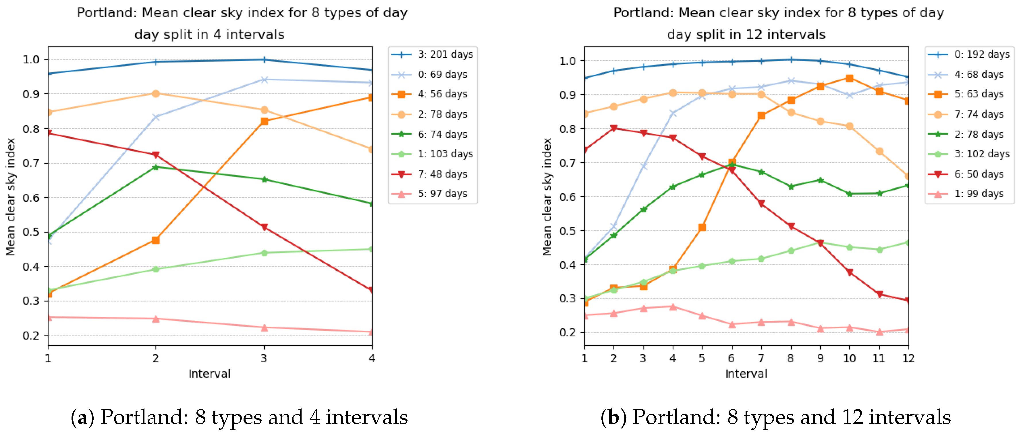
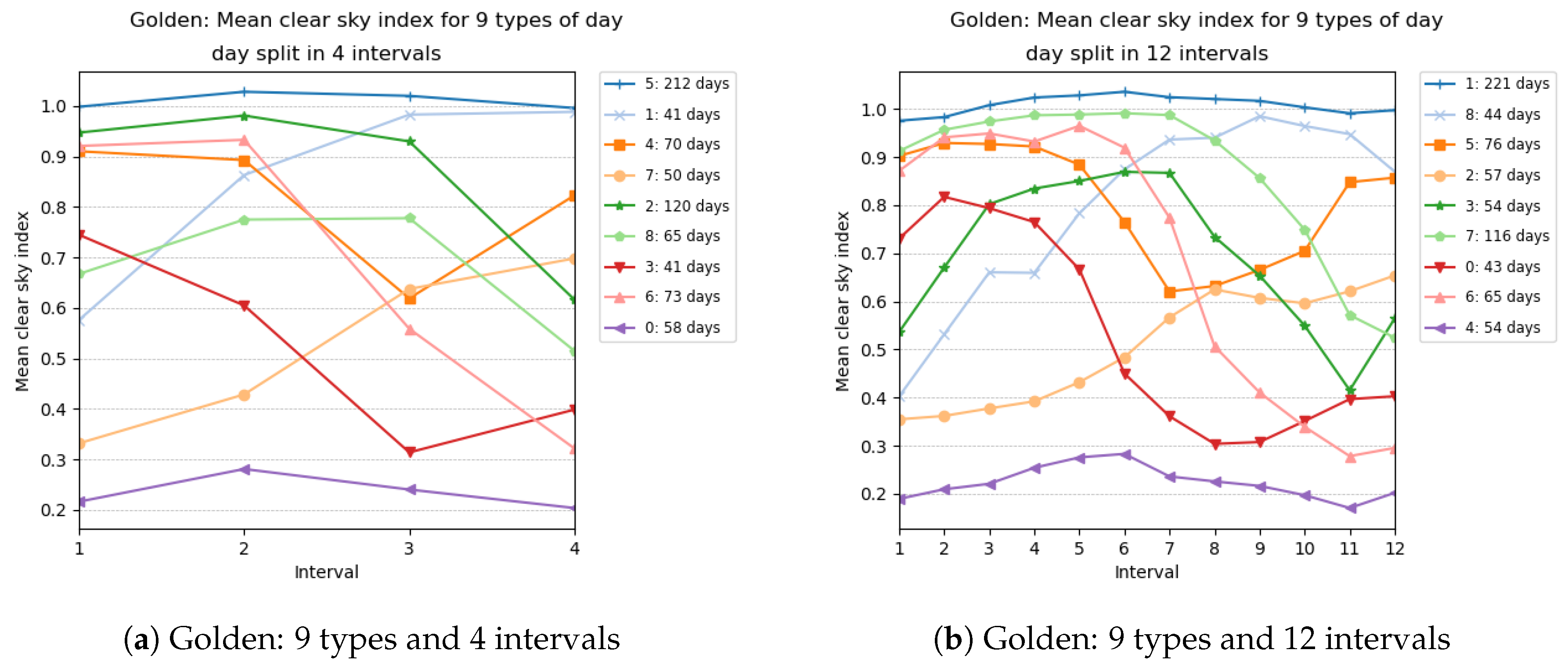
We illustrate in Figure 4 and Figure 5 the types obtained for selected numbers of clusters (in other words, selected sizes of ) and selected number of intervals. Each graphic in these figures reports the centroids of the clusters obtained. The numbering of the clusters changes at each run, but by looking at the centroids obtained, it is often possible to map the clusters obtained with different number of intervals. For instance, the cluster (type) numbered 3 in Figure 4a has a centroid with coordinates close to 1, which represents days where the clear sky index is close to 1 all day long. Such clear sky days are grouped in cluster 0 in Figure 4b, whose centroid has coordinates close to 1. Similarly, type 0 in Figure 5a can be mapped to type 4 in Figure 5b and represents days with heavy clouds.
As for the distributions , , , we use the empirical distributions of the clear sky index of the days in cluster in the training set and view them as the ground truth for the day type . For illustration purposes, we display in Figure 6 the distributions when there are types of days and the day is partitioned into intervals (this implies that there are actually three distinct distributions for each day type).
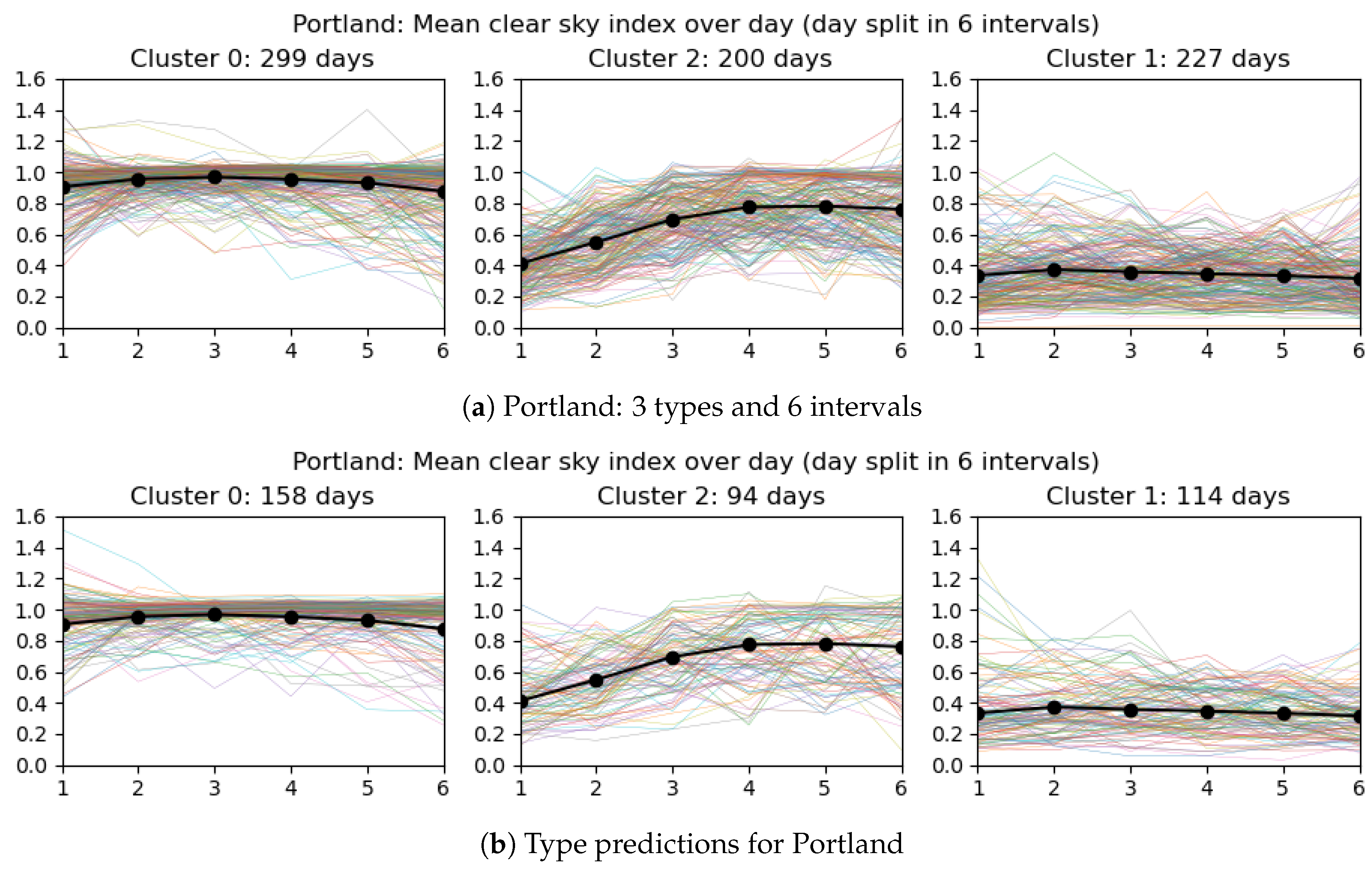
Once clusters have been identified, we predict the types of the days present in the testing set (which will be used in the experiments). We illustrate in Figure 7 the predictions obtained for Portland when there are three day types (clusters) and the day is split into six intervals. In the practical use of the model, the data of next day are obviously not known exactly. A proxy for it is given by weather predictions. Assuming that some hourly prediction of cloudiness is available from the weather service, the representative values for each interval can be determined, to serve as the basis for the day type prediction. If hourly predictions are not available, coarser information can be used in conjunction with a model with fewer intervals.
4.2. Energy Consumers
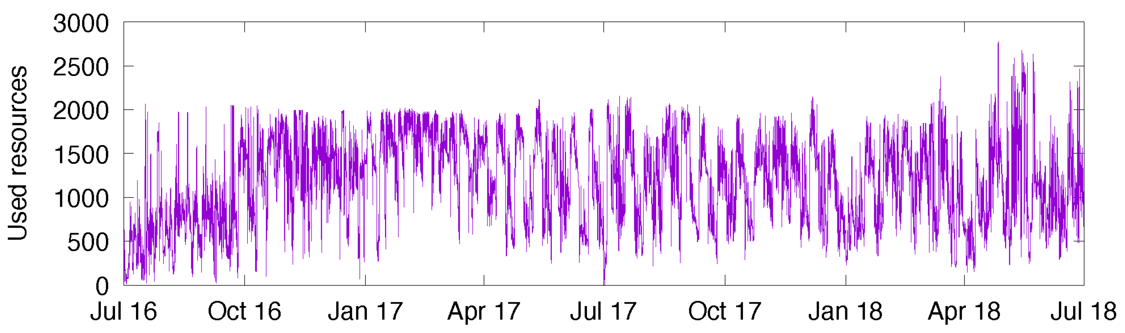
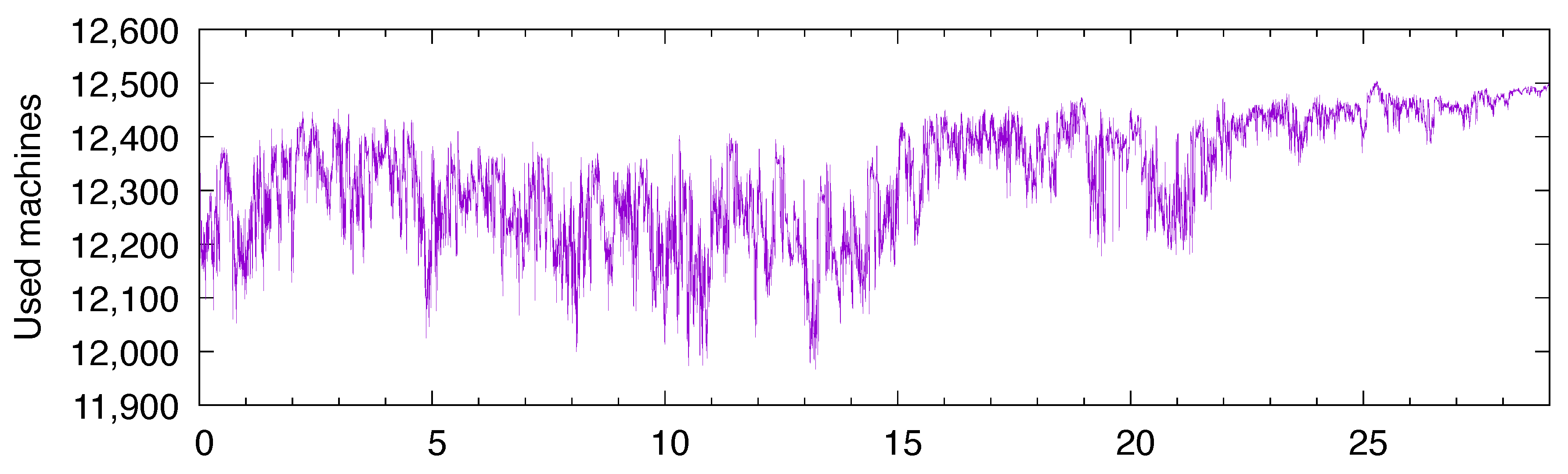
The solar energy collected by photovoltaic sources and stored in batteries is used to power a computing cluster. To simulate the energy consumption of a computing cluster, we rely on traces of two real clusters. The first cluster, called NEF [27], is used internally at Inria for research purposes. The workload trace that we have covers the workload experienced over a period of two years (from July 2016 until June 2018—this trace was captured by Inria’s IT staff in July 2018 and we got exclusive rights to use it after screening by Inria’s General Data Protection Regulation officer). The second cluster is part of a larger Google computing cluster, used mostly internally by Google employees, but it also runs jobs for clients. The detailed workload description can be found in [25]. This trace covers a period of 29 days in May 2011. For each of the clusters, we first computed the number of resources/machines used over time, and then integrated that number every minute (since our solar model has the minute as its unit of time). The energy consumption per minute is a function of this integrated workload; see (4). Figure 8 depicts the workload of NEF, and Figure 9 depicts that of the Google cluster.
To suit our experiments, we had to pre-process these traces in order to give them the same order of magnitude. To begin with, the Google trace clearly fluctuated between around 11,900 and around 12,500 resources. With this fluctuation being small relative to the total, the datacenter might be seen as having an almost constant consumption. In order to give more variability to the trace, we have subtracted the baseline value 11,900. As a result, the workload fluctuates between 0 and 600 approximately. In comparison, the NEF trace fluctuates between 0 and 2000 most of the time.
The global characteristics of these traces are summarized in Table 2. Observe that the unit used is relevant for the minute-based model.
5. Experiments
We now present the experimental setup and the results of these experiments.
5.1. Synthetic Solar Traces
In our experiments, we have used the models of solar sources described in Section 2.
The sources we call “sinusoidal” are defined by the clear sky irradiance model in Section 2.2 with the clear sky irradiance given by (2). We have used astronomical data and recorded weather data to define their parameters. These sources generate a deterministic trajectory.
The models described in Section 2.3 are denoted “daily” and “hourly”. To find their parameters, we have used the training data to form the empirical distributions of monthly daylight irradiance, or monthly hourly irradiance. The generation of one trajectory consists of drawing one sample from these distributions every day (for the daily sources) or every hour (for the hourly sources).
For our new forecast-based source defined in Section 4.1, which we call “synthetic”, we have used the day type predictions of the testing data and the distributions for and , for generating trajectories for given days of the year.
5.1.1. Trajectories
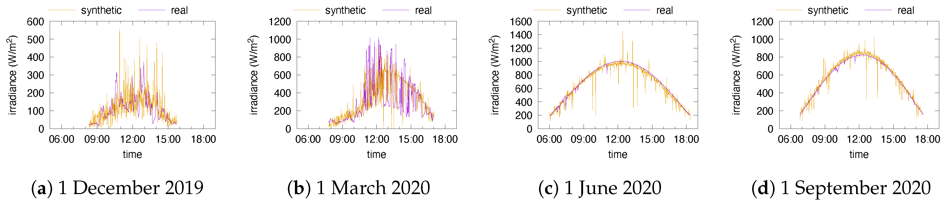
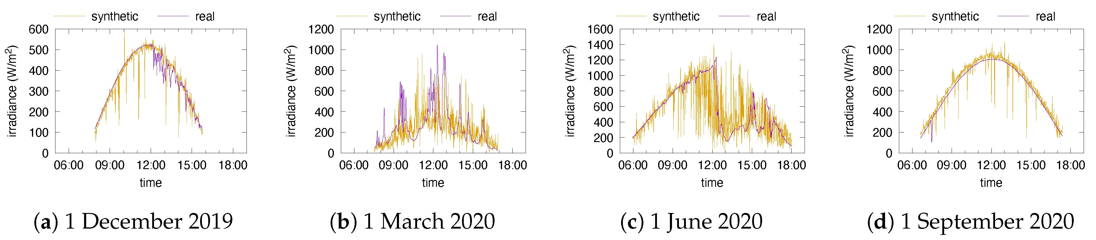
One first step when validating a model is to generate synthetic traces and compare them with reality. Figure 10 and Figure 11 depict the daily global irradiance of several days together with synthetic data for these days. We have not represented trajectories of daily and hourly sources, since their piecewise-constant shape makes them look very different from real traces. Likewise, the sinusoidal curves may look similar to the real ones on clear days, but the maximal irradiance usually differs because of the averaging of the cloudiness over one month.
From Figure 10 and Figure 11 we conclude that the clustering apparently identifies correctly some trends in the weather: perfect days on 1 June 2020 and 1 September 2020 in Portland and 1 September 2020 in Golden; perfect mornings and then a degradation on 1 December 2019 and 1 June 2020 in Golden. On the other hand, we also see the effect of the irradiance distributions attached to clusters, coupled with the re-sampling of irradiances at each minute: even on perfect days, the synthetic irradiance is irregular. These irregularities may be smoothed out by the buffering in the battery though.
5.1.2. Global Characteristics
In a second step, we examine the global, longer-term characteristics of the sources. Consistent with our premises that stationarity is difficult to exhibit in the irradiance phenomenon, we do not favor the spectral analysis of the signal obtained, since this is a feature of wide-sense stationary signals. Instead, we settle for averages of the power over given periods. The average yearly power generated by the sources we use are given in Table 3. For the benchmark situation, this average is computed over the testing year. The synthetic source selected is the one with clusters and intervals. The value displayed is the empirical average of 36 samples, together with the half-width of the 95% confidence interval. The source called “pure sinusoidal” is the one given by (2). The one called “damped sinusoidal” considers the clear-sky index of (3) in addition.
Table 4 and Table 5 display the average power generated by different sources computed over each month. For sinusoidal sources, the cloudiness values have been taken from Table 1 (line “Denver, completed”). Discrepancies between averaged yearly powers may be explained by small variations in the number of days in the year (leap days) or days missing in the records due to malfunctioning of the recording equipment.
The purpose of these tables is to illustrate several features of the data. First, the monthly variation is obvious, but it is worth stressing the observation that the ratio of the most sunny month over the least sunny one may be larger than four. Second, the variations in one year (testing) in relation to the average of the two previous ones (training) are sometimes large on a monthly basis, although they usually smooth out for the whole year. The four first lines contain the real data, split over training/testing and with the presentation of statistics restricted to daylight hours (tagged with “day”). This allows one to assess that the irradiance does vary over the months, not just as a consequence of varying durations of daylight time over the year.
5.2. Workload
In simulations, we used two real traces that have been described in Section 4.2.
5.3. Datacenter
The characteristics of the datacenter are as follows. There are computing nodes, which is a number larger than the maximum number of resources used in the real traces we used (see Figure 8 and Figure 9). The power consumption values of these computing nodes (see Equation (4)) are taken as W and W. A rationale for this choice is that values W and W have been measured on Grid5K platform nodes in 2015 [28]. The values we chose account for an improvement in hardware consumption equivalent to roughly running twice as many nodes with the same energy.
Battery capacity in experiments will range from 1 to 10 GJ, that is, less than what is necessary to store 1 day of energy input or consumption. Indeed, for a solar source of mean power 150 W/m over a day and a PV panel surface of 1200 (efficient) m, the daily energy input is GJ. The panel surface will range from 1200 to 12,000 m.
These values are chosen so that the proportions of time the battery is empty or full are not trivially close to 0 or 1: in those situations, the complexity of the solar input model is irrelevant to predict the correct value.
5.4. Results
5.4.1. First experiments
For each city and for each energy source, we performed a first series of simulations considering either of the two consumers and various battery capacities and surface areas of photovoltaic panels. The six settings presented in Table 6 were used.
For each simulation we recorded the empirical distribution of the battery level. We only report in the following on the values of two performance metrics, namely, the percentage of time that the battery was full and the percentage of time that the battery was empty. We do not name these metrics “probabilities” because they do not result from some stationary phenomenon. When the source is random in nature, the percentage is obtained by averaging 36 independent replications. Occasionally, we display the corresponding 95% confidence interval.
Figure 12 and Figure 13 display the performance metrics obtained for the cities of Portland and Golden, respectively, when the energy sources described in Section 2.3, Section 2.4 and Section 4.1 are used, and for a single pair of values for battery capacity and panel surface.
Each point in the figure represents the performance of a single energy source in terms of the full/empty battery proportion. The naming of the source is that of Section 5.1. Our forecast-based model described in Section 4.1 has 180 configurations according to the considered numbers of day types and day intervals. All configurations with the same number of day type (i.e., number of clusters) use the same point shape/color and are denoted by their number of clusters; thus, there are 12 similar points with the same label, one for each possible number of day intervals.
For a given energy source model, the closer its point to that of the benchmark, the better it is, as this suggests the energy model captures the essential features needed for the use case. It is clear from the graphs displayed in Figure 12 and Figure 13 that the “daily”, “hourly” and “sinusoidal” models fail to predict the performance in terms of the percentage of time when the battery is full/empty. Therefore, they should not be used for the purpose of managing a datacenter fed by photovoltaic panels. Instead, our energy model with any of its 180 configurations yields a performance very similar to that achieved by the benchmark, making it a good candidate for this use case scenario.
The performance metrics are further discussed in Appendix A (for the percentage of time when the battery is empty) and Appendix B (for the percentage of time when the battery is full). A close look at the individual values reported in each of the graphs displayed in Figure A1, Figure A2, Figure A3, Figure A4 does not allow one to identify the configuration for which our forecast-based energy source model achieves the closest performance to the benchmark’s regardless of the experimental setting. In the next section we will present our approach to select the best configuration.
5.4.2. Selection of Most Promising Configurations
To assess which out of all 180 configurations considered in our energy model best approaches the benchmark, we consider four selection criteria, as explained next. Each configuration has been tested in six experimental settings yielding two performance metrics. In total, we have 12 pairs of values (benchmark, model) for each configuration. We compute
- The maximum relative distance among the pairs of values (benchmark, model).
- The average relative distance over all pairs.
- The root mean square distance over all pairs.
- A weighted sum of the previous three criteria.
This last criterion deserves some words of explanation. Whereas the maximum relative distance and the average relative distance are of the same order of magnitude as the relative distance between the benchmark and model, the root mean square distance has the same order of magnitude as the standard deviation of the benchmark values. The weighted sum is such that all three terms have the same order of magnitude.
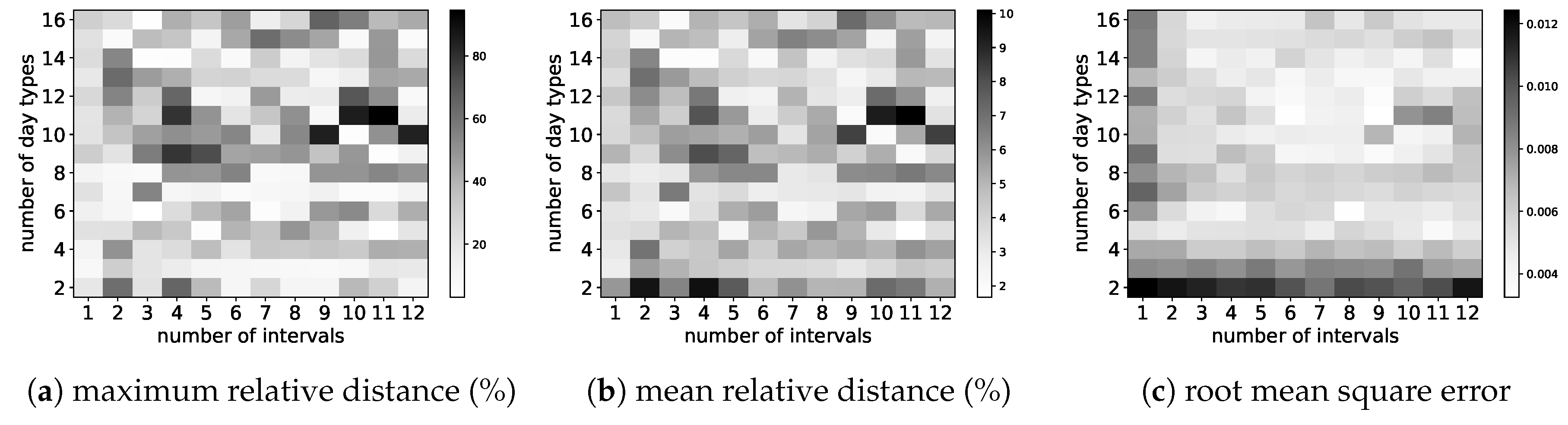
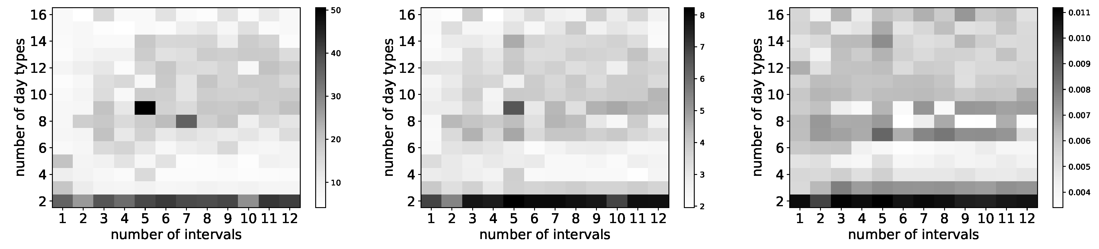
The selection criterion is to choose the configuration having the smallest value. In Figure 14, we report graphically the values of the first three criteria obtained for all 180 configurations for Portland. The same for Golden are displayed in Figure 15.
As we want the configuration in terms of the number of day intervals and the number of day types that achieves the smallest distances, we need to look for those configurations with the brightest colors in each graphic. Our observations are as follows. First, it came as a surprise to us to see huge differences between neighboring configurations. For instance, from Figure 14a we observe that for Portland the maximum relative distance drastically changes when the number of day intervals changes from 9 to 10 for a number of day types equal to 10 (or 11, same observation). The value goes from 84.79 to 4.85 (and from 9.13 to 85.40 when there are 11 day types). Second, we observe an interesting trend in Figure 15a where configurations in the center of the graphics achieve worse maximal relative distances than configurations at the periphery. This is observed also in Figure 15b, although to a lesser extent. There are no clear trends in any of the graphics of Figure 14. Third, many configurations are candidates for being the best achiever, as they have bright spots in all three graphics for each city. To identify these with certainty, we resorted to a ranking analysis.
We first discuss the case of the city of Portland. Table 7 lists the top 10 configurations according to the sum of all three criteria. Configuration is ranked first according to both the maximum/mean relative distance and the sum of three criteria, and ranked eightth according to the root mean square distance. The fact that this configuration yields small errors according to the three criteria is confirmed visually in Figure 14, although the neighboring configurations are not as good. This configuration with 5 day types and 11 day intervals was selected as the most promising one (for Portland) and was used for further experiments.
We then followed the same approach for the city of Golden. Table 8 displays the top 10 configurations with respect to the sum of all criteria, together with the individual ranking for each of them. When adding criteria about a small maximum and small mean relative distance, only three remain: configurations , and . None of these configurations are in the top 10 according to the lowest root mean square error achieved in the experiments. Among the three finalists, we selected the configuration with 16 day types and 2 day intervals as the most promising one (for Golden), since it is ranked first according to the maximum relative distance criterion (and the sum criterion) and third according to the mean relative distance criterion. This configuration is ranked 23rd according to the smallest root mean square error criterion; note that the first-ranked configuration has value 0.00339, compared to our choice’s value 0.00426. We used this configuration for further experiments.
By selecting for each city the configuration that achieved the smallest maximum relative distance in the first series of experiments, we are confident of the robustness of our energy model with this configuration.
For completeness, we report in Appendix C the relative distance between the benchmark and model for each performance metric (empty/full battery proportion) achieved by each city’s selected configuration over the first series of experiments.
5.4.3. Further Experiments
To show how the energy models perform on a wider range of parameters, we performed a second series of simulations. For each city and for each of the energy sources, we first varied the battery capacity and fixed the surface area of the photovoltaic panels, and then did the opposite (we fixed the battery capacity and varied the surface area of the photovoltaic panels). For each single simulation we recorded the empirical distribution of the battery level.
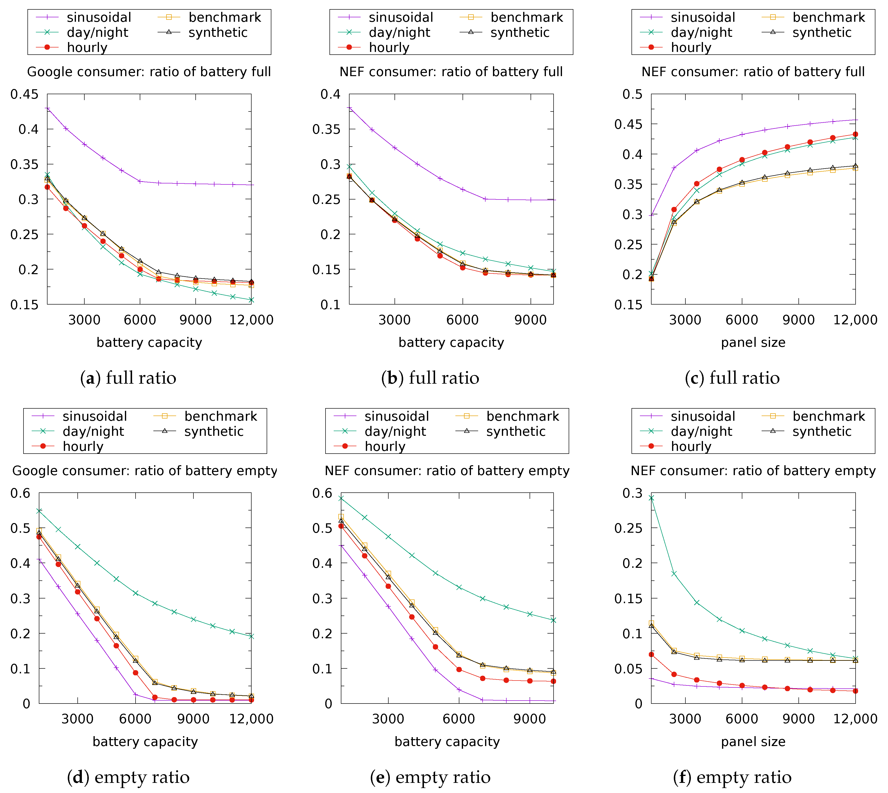
We depict in Figure 16 and Figure 17 the battery full/empty percentages as a function of the battery capacity or alternatively as a function of the panel surface. There are five curves in each figure: one for each of the energy sources considered, namely, sinusoidal, daily and hourly (described in Section 2.3 and Section 2.4); benchmark (which corresponds to the global irradiance measured during a one-year period [20,21]); and synthetic (which corresponds to our forecast-based energy model described in Section 4.1 with 5 day types and 11 day intervals in the case of Portland, and with 16 day types and 2 day intervals in the case of Golden). It is obvious that the performance achieved when using our forecast-based sources matches perfectly the benchmark performance. This strengthens the previous observations that we made with experiments and confirms the supremacy of our energy models over the other models in the use case at hand.
6. Conclusions
We have considered in this paper the problem of modeling the solar energy on a scale fine enough to be useful for the analysis of solar-powered computer systems. We have proposed a novel way of generating samples of solar irradiance for future days, based on the knowledge of the weather outlook. This method involves clustering a recorded trace of irradiance with easily computed features. These features are based on the clear sky index instead of the clear sky irradiance. We demonstrate, through simulations, that our new solar source performs better in predicting battery shortage and overflows than previously proposed models, when feeding a datacenter submitted to a workload obtained from real traces.
The next steps in the analysis will aim at confirming the robustness of our approach by confronting the forecast-based source with more energy consumption models (i.e., datacenter workload models), and fitting the model to more solar data. With more experimental results, we will investigate further the question of selecting the proper configuration of clusters and intervals for our model. We also plan to develop a queuing-theoretic analysis and a control-theoretic analysis of datacenters, based on our new solar source model. For this purpose, a (semi)Markovian representation of the clear sky index process may prove handy.
The data and the programs used in this study will, after review, be made available through gitlab.
Author Contributions
Conceptualization, S.A. and A.J.-M.; data curation, S.A. and A.J.-M.; formal analysis, S.A. and A.J.-M.; investigation, S.A. and A.J.-M.; methodology, S.A. and A.J.-M.; software, S.A. and A.J.-M.; validation, S.A. and A.J.-M.; visualization, S.A. and A.J.-M.; writing—original draft, S.A. and A.J.-M.; writing—review and editing, S.A. and A.J.-M. All authors have read and agreed to the published version of the manuscript.
Funding
This research received no external funding.
Conflicts of Interest
The authors declare no conflict of interest.
Abbreviations
The following abbreviations are used in this manuscript:
| DC | Datacenter |
| DM | Datacenter manager |
| PV | Photovoltaic |
Appendix A. Empty Ratio: Detailed Performance
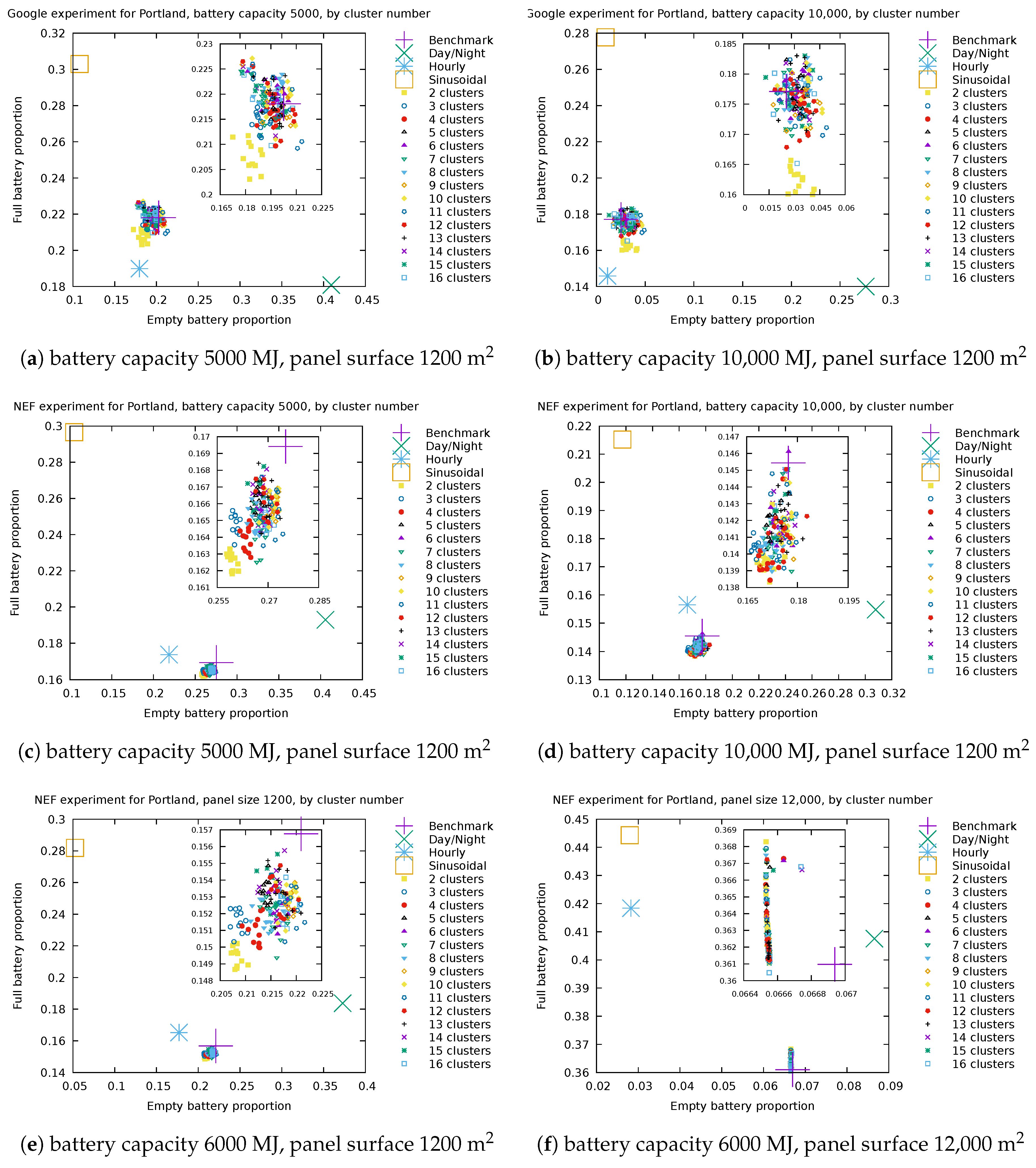
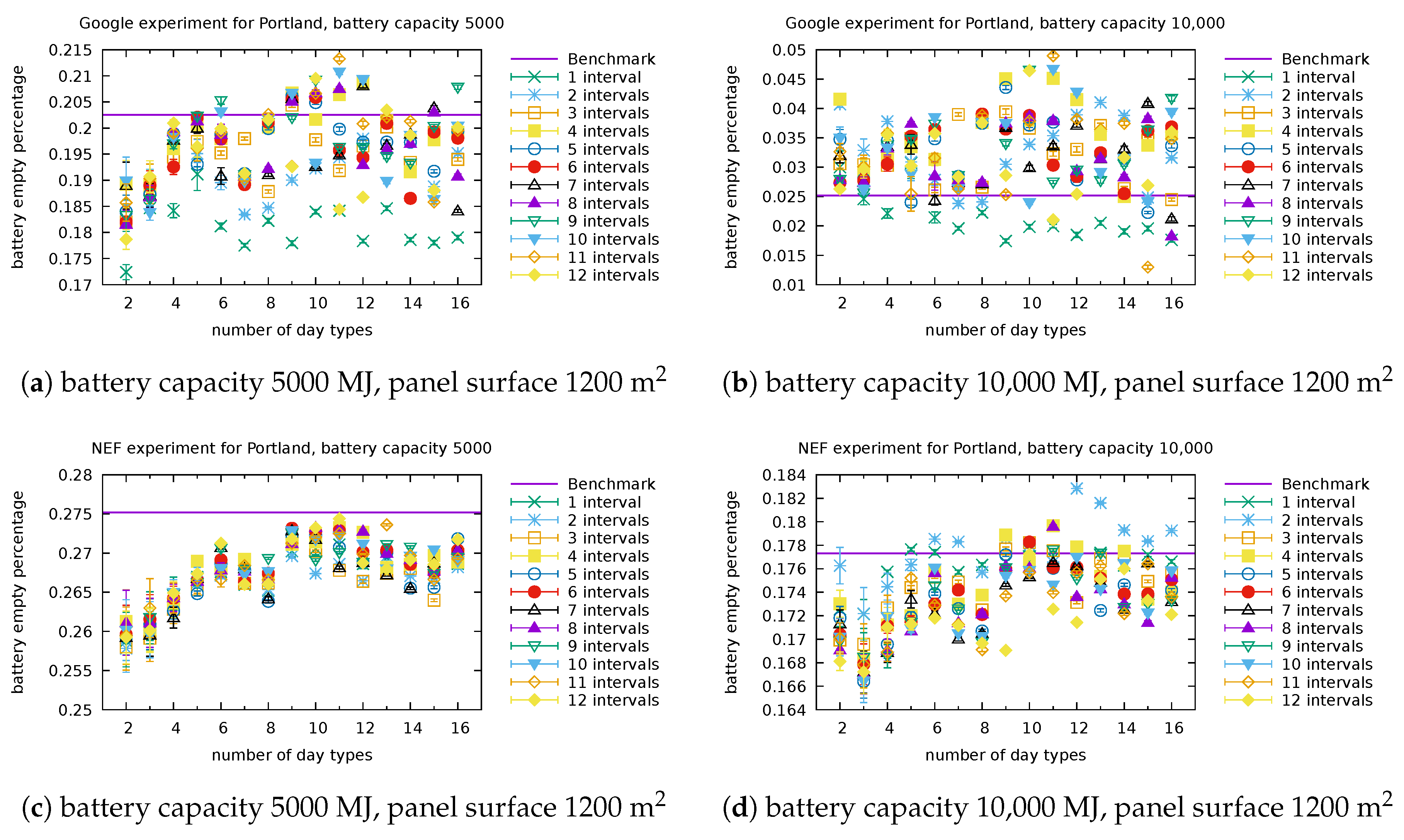
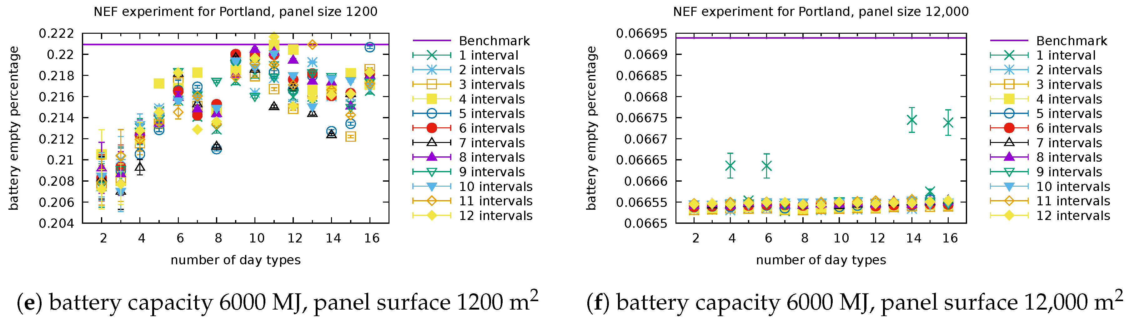
The percentage of time when the battery is empty is depicted with its 95% confidence intervals in Figure A1 (for Portland) and Figure A2 (for Golden) with NEF/Google consumers and for several settings of the battery capacity and panel surface. We observe that some configurations of our energy models perform better than others in a single setting, but this changes from one setting to another. When the configuration has a small number of types, equal to 2 or 3 (or even 4), the confidence intervals are larger and the performance metrics farther from the benchmark than the other configurations in most cases. We conclude from these figures that no configuration in terms of number of day types and number of day intervals is always the best and other selection criteria should be determined to select the most promising configurations. Nevertheless, we believe that one has the possibility to use any of the configurations (except for 2–4 day types) and still be confident in the accuracy of the results.
Figure A1.
Empty ratio, Portland: Detailed performance of our model for several settings of the battery capacity and panel surface with Google consumer (a,b) and NEF consumer (c–f).
Figure A1.
Empty ratio, Portland: Detailed performance of our model for several settings of the battery capacity and panel surface with Google consumer (a,b) and NEF consumer (c–f).


Figure A2.
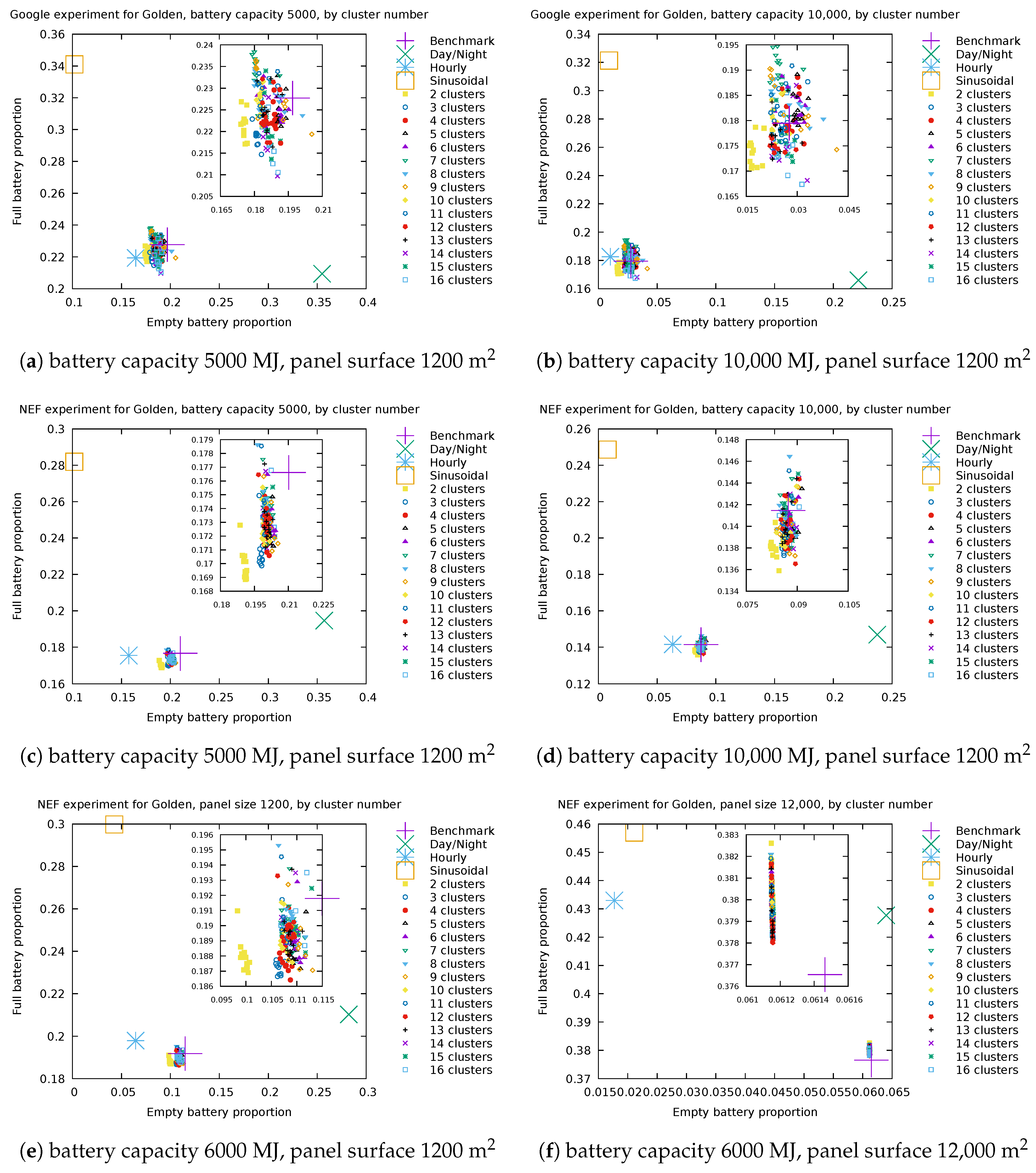
Empty ratio, Golden: Detailed performance of our model for several settings of the battery capacity and panel surface with Google consumer (a,b) and NEF consumer (c–f).
Figure A2.
Empty ratio, Golden: Detailed performance of our model for several settings of the battery capacity and panel surface with Google consumer (a,b) and NEF consumer (c–f).

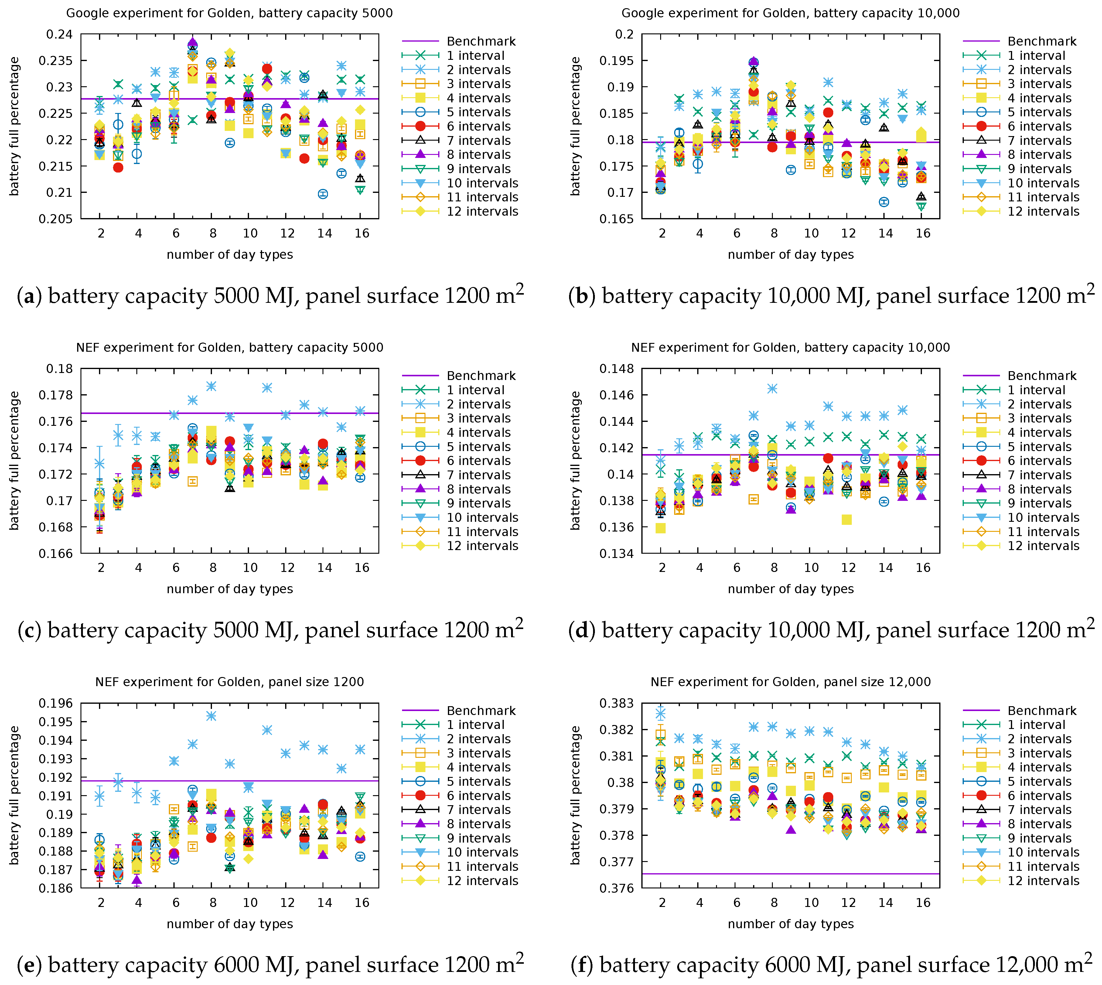
Appendix B. Full Ratio: Detailed Performance
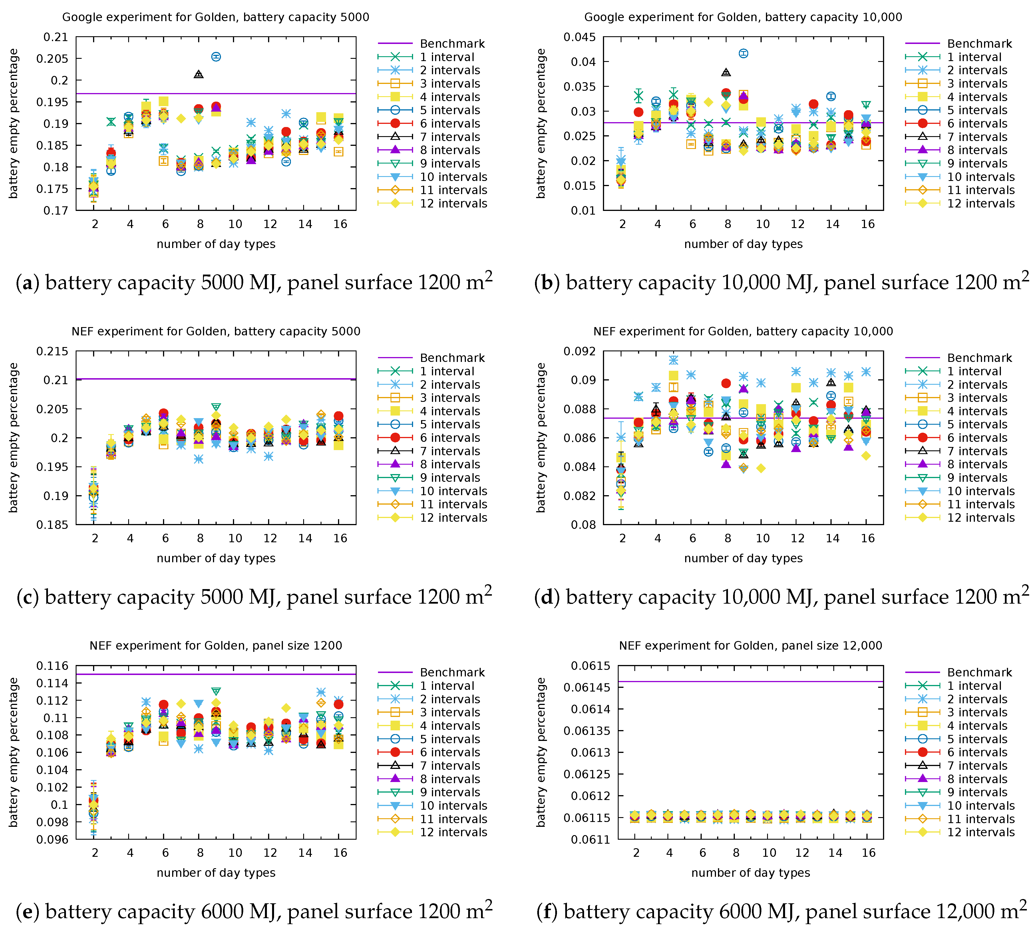
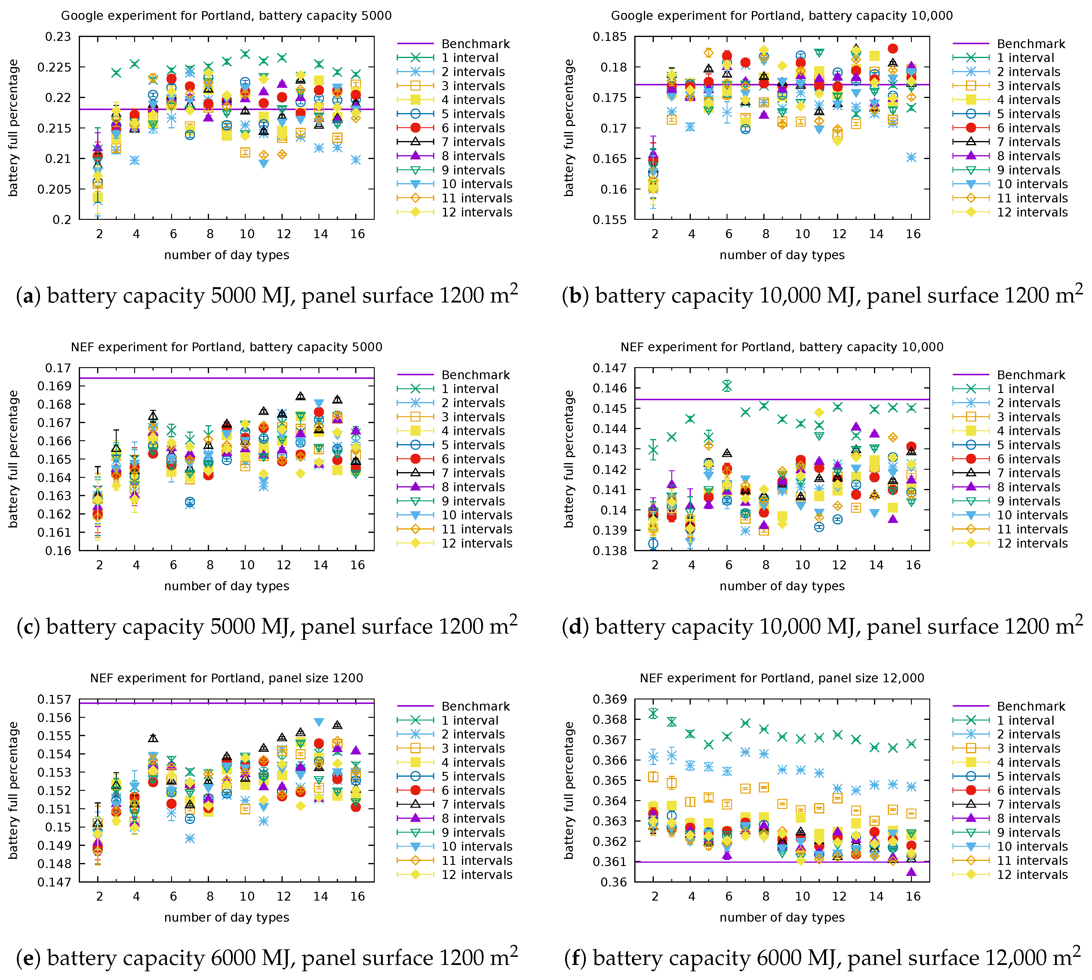
Similarly to what was done in Appendix A, the percentage of time when the battery is full is depicted with its 95% confidence intervals in Figure A3 (for Portland) and Figure A4 (for Golden) with NEF/Google consumers and for several settings of the battery capacity and panel surface. We are again unable to visually identify with certainty the best model configuration. The observations made in Appendix B are valid here.
Figure A3.
Full ratio, Portland: Detailed performance of our model for several settings of the battery capacity and panel surface with Google consumer (a,b) and NEF consumer (c–f).
Figure A3.
Full ratio, Portland: Detailed performance of our model for several settings of the battery capacity and panel surface with Google consumer (a,b) and NEF consumer (c–f).

Figure A4.
Full ratio, Golden: Detailed performance of our model for several settings of the battery capacity and panel surface with Google consumer (a,b) and NEF consumer (c–f).
Figure A4.
Full ratio, Golden: Detailed performance of our model for several settings of the battery capacity and panel surface with Google consumer (a,b) and NEF consumer (c–f).

Appendix C. Relative Distance Achieved by the Selected Configurations
We use the labels introduced in Table 6 to refer to the settings used in the first series of experiments. The relative distance between the benchmark and the model is reported in Table A1 for the selected configurations for each city. In addition, we report the mean obtained over all six values regarding the same performance metric.

Table A1.
Relative distance (in percentage) in the first series of experiments.
| City | Types | Intervals | Metric | G5000 | G10000 | N5000 | N10000 | N1200 | N12000 | Mean |
|---|---|---|---|---|---|---|---|---|---|---|
| Portland | 5 | 11 | empty | 3.17 | 1.07 | 2.11 | 1.33 | 1.97 | 0.59 | 1.70 |
| full | 2.36 | 2.95 | 1.30 | 1.51 | 1.45 | 0.23 | 1.63 | |||
| Golden | 16 | 2 | empty | 3.82 | 3.01 | 4.14 | 3.92 | 3.54 | 0.51 | 3.15 |
| full | 0.60 | 3.37 | 0.75 | 0.21 | 0.16 | 1.06 | 1.03 |
References
- Kong, F.; Liu, X. A Survey on Green-Energy-Aware Power Management for Datacenters. ACM Comput. Surv. 2014, 47. [Google Scholar] [CrossRef]
- Cioara, T.; Anghel, I.; Antal, M.; Crisan, S.; Salomie, I. Data center optimization methodology to maximize the usage of locally produced renewable energy. In Proceedings of the SustainIT: Sustainable Internet and ICT for Sustainability, Madrid, Spain, 14–15 April 2015; pp. 1–8. [Google Scholar] [CrossRef] [Green Version]
- Liu, Z.; Chen, Y.; Bash, C.; Wierman, A.; Gmach, D.; Wang, Z.; Marwah, M.; Hyser, C. Renewable and Cooling Aware Workload Management for Sustainable Data Centers. SIGMETRICS Perform. Eval. Rev. 2012, 40, 175–186. [Google Scholar] [CrossRef] [Green Version]
- Goiri, I.; Katsak, W.; Le, K.; Nguyen, T.D.; Bianchini, R. Designing and Managing Data centers Powered by Renewable Energy. IEEE Micro 2014, 34, 8–16. [Google Scholar] [CrossRef]
- Politaki, D.; Alouf, S. Stochastic Models for Solar Power. In Proceedings of EPEW: European Performance Evaluation Workshop; Springer: Berlin/Heidelberg, Germany, 2017; Volume 10497, pp. 282–297. [Google Scholar] [CrossRef] [Green Version]
- Dimitriou, I.; Alouf, S.; Jean-Marie, A. A Markovian Queueing System for Modeling a Smart Green Base Station. In Proceedings of EPEW: European Performance Evaluation Workshop; Springer: Berlin/Heidelberg, Germany, 2015; Volume 9272, pp. 3–18. [Google Scholar] [CrossRef] [Green Version]
- Neglia, G.; Sereno, M.; Bianchi, G. Geographical Load Balancing across Green Datacenters: A Mean Field Analysis. ACM SIGMETRICS Perform. Eval. Rev. 2016, 44, 64–69. [Google Scholar] [CrossRef]
- Fourneau, J. Modeling Green Data-Centers and Jobs Balancing with Energy Packet Networks and Interrupted Poisson Energy Arrivals. SN Comput. Sci. 2020, 1, 1–28. [Google Scholar] [CrossRef] [Green Version]
- Dave, J.V.; Halpern, P.; Myers, H.J. Computation of Incident Solar Energy. IBM J. Res. Dev. 1975, 19, 539–549. [Google Scholar] [CrossRef]
- Bird, R.E.; Hulstrom, R.L. Review, Evaluation, and Improvement of Direct Irradiance Models. J. Sol. Energy Eng. 1981, 103, 182–192. [Google Scholar] [CrossRef]
- Bird, R.E.; Hulstrom, R.L. A Simplified Clear Sky Model for Direct and Diffuse Insolation on Horizontal Surfaces; Technical Report SERI/TR-642-761; Solar Energy Research Institute: Golden, CO, USA, 1981.
- Piedallu, C.; Gégout, J.C. Multiscale computation of solar radiation for predictive vegetation modelling. Ann. For. Sci. 2007, 64, 899–909. [Google Scholar] [CrossRef] [Green Version]
- Sun, S.; Kazhamiaka, F.; Keshav, S.; Rosenberg, C. Using Synthetic Traces for Robust Energy System Sizing. In Proceedings of the e-Energy ’19: The Tenth ACM International Conference on Future Energy Systems, Phoenix, AZ, USA, 25–28 June 2019. [Google Scholar]
- Miozzo, M.; Zordan, D.; Dini, P.; Rossi, M. SolarStat: Modeling Photovoltaic Sources through Stochastic Markov Processes. In Proceedings of the 2014 IEEE International Energy Conference, Cavtat, Croatia, 13–16 May 2014; pp. 688–695. [Google Scholar] [CrossRef] [Green Version]
- Suehrcke, H.; McCormick, P. The frequency distribution of instantaneous insolation values. Sol. Energy 1988, 40, 413–422. [Google Scholar] [CrossRef]
- Jurado, M.; Caridad, J.; Ruiz, V. Statistical distribution of the clearness index with radiation data integrated over five minute intervals. Sol. Energy 1995, 55, 469–473. [Google Scholar] [CrossRef]
- Ghiassi-Farrokhfal, Y.; Keshav, S.; Rosenberg, C.; Ciucu, F. Solar Power Shaping: An Analytical Approach. IEEE Trans. Sustain. Energy 2015, 6, 162–170. [Google Scholar] [CrossRef]
- Gu, L.; Fuentes, J.D.; Garstang, M.; Tota da Silva, J.; Heitz, R.; Sigler, J.; Shugart, H.H. Cloud modulation of surface solar irradiance at a pasture site in southern Brazil. Agric. For. Meteorol. 2001, 106, 117–129. [Google Scholar] [CrossRef]
- Gueymard, C.A. A review of validation methodologies and statistical performance indicators for modeled solar radiation data: Towards a better bankability of solar projects. Renew. Sustain. Energy Rev. 2014, 39, 1024–1034. [Google Scholar] [CrossRef]
- Vignola, F.; Andreas, A. University of Oregon: GPS-Based Precipitable Water Vapor (Data); Report DA-5500-64452; NREL: Golden, CO, USA, 2013. [CrossRef]
- Andreas, A.; Stoffel, T. NREL Solar Radiation Research Laboratory (SRRL): Baseline Measurement System (BMS); Report DA-5500-56488; NREL: Golden, CO, USA, 1981. [CrossRef]
- ptaff.ca. Sunrise, Sunset Daylight in a Graph. Available online: https://ptaff.ca/soleil/ (accessed on 20 October 2020).
- weatherexplained.com. 2001 Portland, Oregon (PDX)—Average, Low, World, Daily, High, Snowfall, Days, Normals, Means, and Extremes. Available online: http://www.weatherexplained.com/Vol-5/2001-Portland-Oregon-PDX.html (accessed on 28 October 2020).
- weatherexplained.com. 2001 Denver, Colorado (DEN)—Average, Low, World, Daily, High, Snowfall, Days, Normals, Means, and Extremes. Available online: http://www.weatherexplained.com/Vol-2/2001-Denver-Colorado-DEN.html (accessed on 28 October 2020).
- Reiss, C.; Wilkes, J.; Hellerstein, J.L. Google Cluster-Usage Traces: Format + Schema; Technical Report; Revised 2014-11-17 for Version 2.1; Google Inc.: Mountain View, CA, USA, 2011; Available online: https://github.com/google/cluster-data/blob/master/ClusterData2011_2.md (accessed on 26 November 2020).
- Pedregosa, F.; Varoquaux, G.; Gramfort, A.; Michel, V.; Thirion, B.; Grisel, O.; Blondel, M.; Prettenhofer, P.; Weiss, R.; Dubourg, V.; et al. Scikit-learn: Machine Learning in Python. J. Mach. Learn. Res. 2011, 12, 2825–2830. [Google Scholar]
- Clusters Home. Available online: https://wiki.inria.fr/ClustersSophia/Clusters_Home (accessed on 17 November 2020).
- Khlif, W. How Sustainable Datacenters Can Be? Master Thesis, University Nice Sophia Antipolis, Nice, France, 2015. [Google Scholar]
Figure 1.
Global and clear sky irradiance (left) and clear sky index (right) in Portland for four selected days.
Figure 1.
Global and clear sky irradiance (left) and clear sky index (right) in Portland for four selected days.

Figure 2.
Global and clear sky irradiance (left) and clear sky index (right) in Golden for four selected days.
Figure 2.
Global and clear sky irradiance (left) and clear sky index (right) in Golden for four selected days.

Figure 3.
Principal features of the datacenter model.

Figure 4.
Types of days for Portland.

Figure 5.
Types of days for Golden.

Figure 6.
Distributions of the clear sky index for Golden with 4 day types and 3 day intervals.

Figure 7.
Days’ characteristics and their types for Portland: training data on top, testing data on bottom.
Figure 7.
Days’ characteristics and their types for Portland: training data on top, testing data on bottom.

Figure 8.
Workload (number of used resources) of NEF over time.

Figure 9.
Workload (number of used machines) of the Google cluster over days (May 2011).

Figure 10.
Global irradiance in Portland: measured and synthetic (16 types and 12 intervals).

Figure 11.
Global irradiance in Golden: measured and synthetic (16 types and 12 intervals).

Figure 12.
Portland experiments with Google consumer (a,b) and NEF consumer (c–f).

Figure 13.
Golden experiments with Google consumer (a,b) and NEF consumer (c–f).

Figure 14.
Performance of our forecast-based energy source model for Portland.

Figure 15.
Performance of our forecast-based energy source model for Golden.

Figure 16.
Experiments for Portland: full ratio (a–c) and empty ratio (d–f) as the battery capacity varies ((a,b,d,e) panel surface 1200 m2) and as the panel surface varies ((c,f) battery capacity 6000 MJ).
Figure 16.
Experiments for Portland: full ratio (a–c) and empty ratio (d–f) as the battery capacity varies ((a,b,d,e) panel surface 1200 m2) and as the panel surface varies ((c,f) battery capacity 6000 MJ).

Figure 17.
Experiments for Golden: full ratio (a–c) and empty ratio (d–f) as the battery capacity varies ((a,b,d,e) panel surface 1200 m2) and as the panel surface varies ((c,f) battery capacity 6000 MJ).
Figure 17.
Experiments for Golden: full ratio (a–c) and empty ratio (d–f) as the battery capacity varies ((a,b,d,e) panel surface 1200 m2) and as the panel surface varies ((c,f) battery capacity 6000 MJ).

Table 1.
Cloudiness measures for the two locations used in experiments.
| Location | Year | January | February | March | April | May | June | July | August | September | October | November | December |
|---|---|---|---|---|---|---|---|---|---|---|---|---|---|
| Portland | 5.7 | 6.7 | 6.6 | 6.4 | 6.2 | 5.8 | 5.4 | 3.8 | 4.0 | 4.3 | 5.6 | 6.4 | 6.8 |
| Denver | – | – | 5.0 | 5.3 | 7.2 | 5.6 | 2.5 | – | 2.5 | – | – | – | 2.5 |
| —completed | 3.8 | 5.0 | 5.0 | 5.3 | 7.2 | 5.6 | 2.5 | 2.5 | 2.5 | 2.5 | 2.5 | 2.5 | 2.5 |
Table 2.
Characteristics of the workloads used in the simulation.
| Workload | Duration | Average Number of Resource × Second in a Minute | Average Load |
|---|---|---|---|
| NEF | 730 days | 68,406 | 1,140 |
| 29 days | 25,765 | 429 |
Table 3.
Power of the different solar sources used in experiments (W/m).
| Source | Portland, Oregon | Golden, Colorado |
|---|---|---|
| benchmark | 162.87 | 191.39 |
| pure sinusoidal | 252.51 | 269.18 |
| damped sinusoidal | 157.27 | 215.43 |
| monthly night/day | 168.05 | 193.43 |
| monthly and hourly | 168.19 | 193.40 |
| synthetic | 161.104 ± 0.027 | 188.380 ± 0.052 |
Table 4.
Yearly and monthly average powers for Portland, Oregon (W/m).
| Source | Year | January | February | March | April | May | June | July | August | September | October | November | December |
|---|---|---|---|---|---|---|---|---|---|---|---|---|---|
| real, training (day) | 327 | 140 | 174 | 296 | 322 | 396 | 488 | 485 | 434 | 355 | 268 | 156 | 130 |
| real, testing (day) | 329 | 131 | 237 | 312 | 385 | 384 | 389 | 492 | 482 | 302 | 283 | 179 | 116 |
| real, training | 162 | 54 | 76 | 147 | 180 | 243 | 313 | 304 | 251 | 184 | 119 | 62 | 48 |
| real, testing | 163 | 51 | 103 | 155 | 216 | 236 | 249 | 308 | 279 | 156 | 129 | 72 | 43 |
| Daily, training | 168 | 69 | 76 | 148 | 181 | 244 | 314 | 305 | 253 | 185 | 123 | 63 | 49 |
| Daily, testing | 170 | 71 | 104 | 156 | 217 | 237 | 251 | 310 | 280 | 158 | 130 | 72 | 43 |
| Hourly, training | 168 | 74 | 76 | 148 | 181 | 243 | 314 | 305 | 252 | 185 | 123 | 63 | 49 |
| Hourly, testing | 169 | 76 | 104 | 156 | 216 | 236 | 250 | 308 | 279 | 157 | 130 | 72 | 43 |
| Sinusoidal w/weather | 157 | 67 | 100 | 155 | 219 | 285 | 326 | 368 | 316 | 240 | 144 | 81 | 55 |
Table 5.
Yearly and monthly average powers for Golden, Colorado (W/m).
| Source | Year | January | February | March | April | May | June | July | August | September | October | November | December |
|---|---|---|---|---|---|---|---|---|---|---|---|---|---|
| real, training (day) | 379 | 262 | 324 | 414 | 414 | 382 | 444 | 475 | 437 | 436 | 317 | 267 | 243 |
| real, testing (day) | 387 | 268 | 313 | 387 | 442 | 475 | 466 | 445 | 433 | 412 | 348 | 270 | 241 |
| real, training | 187 | 106 | 144 | 205 | 228 | 228 | 275 | 289 | 248 | 225 | 146 | 110 | 94 |
| real, testing | 191 | 108 | 139 | 192 | 244 | 284 | 288 | 270 | 245 | 212 | 161 | 112 | 94 |
| Daily, training | 193 | 111 | 145 | 207 | 230 | 230 | 277 | 290 | 249 | 226 | 147 | 111 | 95 |
| Daily, testing | 198 | 116 | 140 | 194 | 245 | 285 | 290 | 272 | 247 | 213 | 161 | 113 | 95 |
| Hourly, training | 193 | 117 | 145 | 206 | 229 | 228 | 276 | 289 | 249 | 225 | 147 | 111 | 95 |
| Hourly, testing | 198 | 121 | 139 | 193 | 245 | 284 | 289 | 270 | 246 | 212 | 161 | 112 | 95 |
| Sinusoidal w/weather | 215 | 118 | 159 | 213 | 160 | 300 | 401 | 389 | 346 | 279 | 205 | 147 | 122 |
Table 6.
Settings used in the first series of experiments.
| Label | G5000 | G10000 | N5000 | N10000 | N1200 | N12000 |
|---|---|---|---|---|---|---|
| Battery capacity | 5000 MJ | 10,000 MJ | 5000 MJ | 10,000 MJ | 6000 MJ | 6000 MJ |
| Panel surface | 1200 m | 1200 m | 1200 m | 1200 m | 1200 m | 12,000 m |
| Consumer | NEF | NEF | NEF | NEF |
Table 7.
Top model configurations for Portland: ranking by sum of three criteria.
| Day | Day | maxRelDistance (%) | meanRelDistance (%) | RMSE × 1000 | Sum | ||||
|---|---|---|---|---|---|---|---|---|---|
| Types | Intervals | Value | Rank | Value | Rank | Value | Rank | Value | Rank |
| 5 | 11 | 3.17 | 1 | 1.67 | 1 | 3.75 | 8 | 8.58 | 1 |
| 6 | 3 | 3.83 | 2 | 2.11 | 7 | 4.30 | 20 | 10.24 | 2 |
| 16 | 3 | 4.23 | 3 | 2.06 | 6 | 4.37 | 25 | 10.66 | 3 |
| 14 | 3 | 4.69 | 4 | 1.91 | 3 | 4.07 | 16 | 10.67 | 4 |
| 10 | 10 | 4.85 | 6 | 2.05 | 5 | 4.02 | 14 | 10.92 | 5 |
| 14 | 4 | 5.41 | 8 | 1.89 | 2 | 4.69 | 43 | 11.98 | 6 |
| 9 | 11 | 4.89 | 7 | 2.12 | 8 | 5.02 | 56 | 12.04 | 7 |
| 5 | 5 | 4.70 | 5 | 2.33 | 12 | 5.26 | 69 | 12.29 | 8 |
| 6 | 7 | 5.80 | 9 | 2.30 | 11 | 5.50 | 87 | 13.60 | 9 |
| 7 | 11 | 6.10 | 10 | 2.52 | 15 | 5.63 | 93 | 14.25 | 10 |
Table 8.
Top model configurations for Golden: ranking by sum of three criteria.
| Day | Day | maxRelDistance (%) | meanRelDistance (%) | RMSE × 1000 | Sum | ||||
|---|---|---|---|---|---|---|---|---|---|
| Types | Intervals | Value | Rank | Value | Rank | Value | Rank | Value | Rank |
| 16 | 2 | 4.14 | 1 | 2.09 | 3 | 4.26 | 23 | 10.49 | 1 |
| 5 | 10 | 4.92 | 4 | 2.22 | 8 | 4.23 | 20 | 11.37 | 2 |
| 5 | 7 | 5.34 | 6 | 2.30 | 18 | 4.13 | 19 | 11.77 | 3 |
| 15 | 4 | 4.36 | 2 | 2.46 | 26 | 4.96 | 41 | 11.77 | 4 |
| 15 | 3 | 4.89 | 3 | 2.46 | 27 | 4.62 | 32 | 11.97 | 5 |
| 4 | 10 | 5.43 | 7 | 2.25 | 9 | 4.66 | 33 | 12.34 | 6 |
| 5 | 8 | 5.61 | 9 | 2.34 | 20 | 4.48 | 27 | 12.43 | 7 |
| 4 | 11 | 5.82 | 15 | 2.03 | 2 | 4.62 | 31 | 12.47 | 8 |
| 6 | 6 | 7.04 | 37 | 2.17 | 4 | 3.57 | 4 | 12.78 | 9 |
| 4 | 6 | 5.75 | 11 | 2.28 | 14 | 4.77 | 35 | 12.80 | 10 |
Publisher’s Note: MDPI stays neutral with regard to jurisdictional claims in published maps and institutional affiliations. |
© 2020 by the authors. Licensee MDPI, Basel, Switzerland. This article is an open access article distributed under the terms and conditions of the Creative Commons Attribution (CC BY) license (http://creativecommons.org/licenses/by/4.0/).
Share and Cite
MDPI and ACS Style
Alouf, S.; Jean-Marie, A. Short-Scale Stochastic Solar Energy Models: A Datacenter Use Case. Mathematics 2020, 8, 2127. https://doi.org/10.3390/math8122127
AMA Style
Alouf S, Jean-Marie A. Short-Scale Stochastic Solar Energy Models: A Datacenter Use Case. Mathematics. 2020; 8(12):2127. https://doi.org/10.3390/math8122127
Chicago/Turabian StyleAlouf, Sara, and Alain Jean-Marie. 2020. "Short-Scale Stochastic Solar Energy Models: A Datacenter Use Case" Mathematics 8, no. 12: 2127. https://doi.org/10.3390/math8122127
Note that from the first issue of 2016, this journal uses article numbers instead of page numbers. See further details here.