Article

Study of the Vibrational Predissociation of the NeBr2 Complex by Computational Simulation Using the Trajectory Surface Hopping Method

by
Ernesto García-Alfonso
1,†,‡,
Maykel Márquez-Mijares
1,‡,
Jesús Rubayo-Soneira
1,*,‡,
Nadine Halberstadt
2,‡,
Kenneth C. Janda
3,‡ and
Craig C. Martens
4,‡
1
Instituto Superior de Tecnologías y Ciencias Aplicadas (InSTEC), Universidad de La Habana, Ave. Salvador Allende No. 1110, Entre Boyeros e Infanta, Plaza, La Habana 10400, Cuba
2
Université Toulouse 3 and CNRS, Laboratoire des Collisions, Agrégats et Réactivité, IRSAMC, 118 Route de Narbonne, CEDEX 09, F-31062 Toulouse, France
3
Department of Chemistry, University of California, Irvine, CA 92697, USA
4
University of California, Irvine, CA 92697-2025, USA
*
Author to whom correspondence should be addressed.
Current address: Molecular and Atomic Physics Department, Instituto Superior de Tecnologías y Ciencias Aplicadas, University of Havana, P.C. 6163, Habana 10400, Cuba.
These authors contributed equally to this work.
Mathematics 2020, 8(11), 2029; https://doi.org/10.3390/math8112029
Submission received: 29 October 2020 / Revised: 11 November 2020 / Accepted: 11 November 2020 / Published: 14 November 2020

Abstract

:
The vibrational predissociation of NeBr 2 has been studied using a variety of theoretical and experimental methods, producing a large number of results. It is therefore a useful system for comparing different theoretical methods. Here, we apply the trajectory surface hopping (TSH) method that consists of propagating the dynamics of the system on a potential energy surface (PES) corresponding to quantum molecular vibrational states with possibility of hopping towards other surfaces until the van der Waals bond dissociates. This allows quantum vibrational effects to be added to a classical dynamics approach. We have also incorporated the kinetic mechanism for a better compression of the evolution of the complex. The novelty of this work is that it allows us to incorporate all the surfaces for ( v = 16 , 17 , , 29 ) into the dynamics of the system. The calculated lifetimes are similar to those previously reported experimentally and theoretically. The rotational distribution, the rotational energy and j m a x are in agreement with other works, providing new information for this complex.

1. Introduction

The field of the chemical physics is very broad. Among the main goals of the field is to study the properties and dynamics of molecular systems, including intra-and inter-molecular energy transfer processes leading to dissociation of excited molecules. This goal has been achieved via a large number of theoretical and experimental studies. Time resolved spectroscopic and pump-probe methods, in both the frequency and the time domains, have been especially useful for providing data to test theoretical methods [1,2]. These methods have been applied to the vibrational predissociation of an extensive variety of van der Waals (vdW) complexes composed of three or more atoms with a range of bond energies, atomic masses, and vibrational frequencies. Due to the weakness of the vdW interactions in these systems, the constituents retain their chemical integrity upon complex formation so the energy transfer mechanism can be easily identified and studied at the state-to-state level [3,4,5,6,7,8,9,10,11,12,13,14,15,16]. The NeBr 2 van der Waals molecule has been particularly useful for these studies since the dynamics is on the boarder line for which classical and quantum methods are comparably useful. This allows us to investigate in particular the applicability of the trajectory surface hopping (TSH) method [8,14,15,16]. The TSH method has been widely used [17,18,19,20,21,22,23], demonstrating its validity and efficiency for a variety of molecular dynamics problems. For this study of the vibrational predissociation of NeBr 2 , the diabatic potential energy surfaces are formed by the interaction of the Ne atoms with the v = 16 , 17 , , 29 Br 2 vibrational levels. The couplings between surfaces are provided by the van der Waals potential. The TSH results obtained for NeBr 2 vibrational predissociation are compared to previous work using other methods [8,9,10]. We also implement the “kinetic mechanism” [15] to interpret the results of the TSH simulation. This method considers two mechanism for transferring energy from the vibration of the diatom to the van der Waals modes. The first mechanism corresponds to a direct vibrational predissociation (VP) transfer of the dissociative coordinate. The second mechanism involves preliminary energy transfer to the non-dissociative van der Waals modes, followed by intramolecular vibrational redistribution (IVR). After IVR has taken place, the cluster is cooled by expelling the rare gas atoms, a process called IVR-evaporative cooling (EC). The values of the kinetic rate constants which characterize these elementary steps are determined by fitting the results of the TSH simulation to the analytical expressions for the time evolution of the NeBr 2 concentration. The simplicity of our treatment and its relatively low computational cost will allow it to be extended to systems with more degrees of freedom (e.g., more rare gas atom), thus offering an attractive and different alternative to purely classical treatments.
The paper is organized as follows: in Section 2, we discuss the procedure of the TSH method as well as the computational details. We also describe our implementation of the kinetic mechanism. In Section 3, results are presented and discussed through figures and tables. Section 4 summarizes the conclusions that can be drawn from this work. In the Appendix A, we describe our procedure to compute the transition probabilities in considerable detail.

2. Theory and Methods

We use Jacobi coordinates ( r , R , θ ) to describe the NeBr 2 triatomic complex, with r being the bond length of Br 2 , R the intermolecular distance from the Ne atom to the center of mass of the dihalogen and the angle between r and R vectors. These definitions are shown in Figure 1. Calculations are performed considering total angular momentum null ( J = j + l = 0 ), with j being the angular momentum of Br 2 and l the orbital angular momentum, a well justified constraint while studying photodissociation events.
The classical Hamilton function corresponding to this three degree of freedom model of the complex is written as
H J = 0 = H Br 2 + 1 2 μ Ne Br 2 ( p R 2 + p θ 2 R 2 ) + V i n t ( r , R , θ ) ,
where
H Br 2 = 1 2 μ Br 2 ( p r 2 + p θ 2 r 2 ) + V Br 2 ( r ) ,
V Ne , Br 2 ( r , R , θ ) is the van der Waals interaction between the Ne atom and the Br 2 molecule,
V B r 2 ( r ) = D 1 ( e [ 2 α 1 ( r r ¯ ) ] 2 e [ α 1 ( r r ¯ ) ] ) ,
V Ne B r 2 ( r , R , θ ) = V R ( R 1 ) + V R ( R 2 ) ,
V R ( R ) = D 2 ( e [ 2 α 2 ( R R ¯ ) ] 2 e [ α 2 ( R R ¯ ) ] ) R 1 , 2 2 = R 2 + r 2 / 4 ± r R c o s ( θ ) ,
and V B r 2 is the Morse’s potential between Br-Br atoms. The quantities μ Br 2 = m Br 2 1 + m Br 2 1 and μ Ne Br 2 = m Ne 1 + ( m Br 2 + m Br 2 ) 1 stand for inverse of reduced masses for the Br 2 and NeBr 2 , respectively. The values D 1 , D 2 , α 1 , α 2 , r ¯ and R ¯ are from [24].
For the quantum treatment, we have used as quantum coordinate the Br 2 vibration ( r ) and the other variables are treated as classical coordinates; for our case these are R and θ . A potential energy surface (PES) is defined by a single state of the quantum degree of freedom (r). It is on this surface that the trajectories for the classical degrees of freedom evolve. Quantum transitions are modeled by hops of the trajectories from one surface to another. These are governed by the evolution of the multicomponent time-dependent vibrational wave function | ψ ( t ) .
As we have commented before, our surfaces are diabatic (see Figure 2) and the couplings are provided by the van der Waals potential. This is different from the usual trajectory surface hopping TSH treatment where the transitions occur between electronic adiabatic surfaces, in well defined regions of avoided crossings.

2.1. TSH Method in the Diabatic Representation

For our triatomic system, we can write the Hamiltonian as follow:
H ( r , R , θ ) = H q ( r ) + H e l ( R ) + H i n t ( r , R , θ )
where H q ( r ) is the quantum part depending on the vibrational coordinate r of Br 2 , H c l ( R ) is the Hamiltonian describing the classical degrees of freedom and H i n t ( r , R , θ ) is the interaction operator which couples the quantum and classical degrees of freedom.
In our case, H q ( r ) describes the vibrational motion of Br 2 in the B state,
H q ( r ) = 2 2 μ B r 2 2 r 2 + V B r 2 ( r )
and
H c l ( R ) = p R 2 2 μ N e B r 2 + p θ 2 2 μ N e B r 2 R 2
Finally, H i n t ( r , R , θ ) has the form
H i n t ( r , R , θ ) = p θ 2 2 μ B r 2 r 2 + V N e B r 2 ( r , R , θ )
If we do a variable change | v = | ψ v ( r ) to simplify notation, the averaged Hamiltonian can be written as:
v | H J = 0 | v = ( E v + p R 2 2 μ N e B r 2 ) δ v v + v | V N e B r 2 ( r , R , θ ) | v + p θ 2 2 μ B r 2 v | 1 r 2 | v + + p θ 2 2 μ N e B r 2 R 2 δ v v ,
where δ v v = 1 if v = v and 0 if v v is the Kronecker’s delta and E v is the vibrational energy for Br 2 obtained by solving
H ^ B C ψ v ( r ) = E v ψ v ( r ) ,
where H ^ B C operator corresponds to the function H B r 2 ( r ) defined in Equation (6).
We have used Bode’s method [25] for the integration of these equations. This subroutine is very important because we have the Morse potential depending of r , R and θ , and we want to know the averaged effect of r for a vibrational level. It is the source of the PES and the coupling among them is due to non diagonal elements v | H J = 0 | v .
The equations motionscover on the v t h surface are defined as follows (taking into account that | v = | v , v | H J = 0 | v ):
d R d t = v | H J = 0 | v p R = p R μ Ne Br 2
d θ d t = v | H J = 0 | v p θ = p θ v | 1 r 2 | v μ B r 2 + 1 μ N e B r 2 R 2
d p R d t = v | H J = 0 | v R = p θ 2 μ N e B r 2 R 3 v | V N e B r 2 ( r , R , θ ) R | v
d p θ d t = v | H J = 0 | v θ = v | V N e B r 2 ( r , R , θ ) θ | v .
The state vector | ψ ( t ) describing the vibration of Br 2 is obtained by solving the time-dependent Schrödinger equation
i | ψ ( t ) t = [ H q ( r ) + H i n t ( r , R , θ ) ] | ψ ( t ) .
| ψ ( t ) is written as
| ψ ( t ) = v c v ( t ) e i E v t / | v
where the sum is over all v states of H q ( r ) with energy E v , c v ( t ) . The complex variable indicates the amplitude of each vibrational level over the total wave function. This is known as the semiclassical expansion of the electronic wave function. Replacing (Equation (15)) in (Equation (14)), we obtain:
i t v c v ( t ) e i E v t / | v = v c v ( t ) e i E v t / [ H q ( r ) + H i n t ( r , R , θ ) ] | v .
Replacing H q ( r ) | v = E v | v , multiplying v | on the left, and taking into account v v | v = δ v v then yields, respectively:
i e i E v t / c ˙ v ( t ) i E v c v ( t ) = c v ( t ) E v e i E v t / + v c v ( t ) e i E v t / v | H i n t ( r , R , θ ) | v ,
i e i E v t / c ˙ v ( t ) + c v ( t ) E v e i E v t / = c v ( t ) E v e i E v t / + v c v ( t ) e i E v t / v | H i n t ( r , R , θ ) | v ,
and
i c ˙ v ( t ) = v c v ( t ) e i ( E v E v ) t / v | H i n t ( r , R , θ ) | v .
The c v ( t ) coefficients satisfy
c v ˙ ( t ) = i v v | H i n t ( r , R , θ ) | v e [ i ( E v E v ) t / ] c v ( t )
and for each vibrational level we determine the population as follows:
ρ v v ( t ) = c v ( t ) c v * ( t ) ,
where ρ v v ( t ) is the density matrix.
The transition probabilities from the current state v to all other states v v during the time interval Δ t are computed using the surface hopping probability (see Appendix A for more detail):
g v v = 2 Δ t I m c v * ( t ) c v ( t ) e [ i ( E v E v ) t / ] | c v ( t ) | 2 v | H i n t ( r , R , θ ) | v .
The initial conditions for the classical trajectories are selected randomly for a total energy corresponding to the zero-point of the complex NeBr 2 , for a particular vibrational state of the Br 2 molecule. The component of the momentum that is parallel to the quantum state coupling vector is only taken into account to adjust, in order to conserve, the total energy [26,27]. In our case, quantum transitions occur between diabatic surfaces, defined for each vibrational level Br 2 ( B ) . These surfaces are coupled by the NeBr 2 potential. Momenta are adjusted during a surface hop using
P v = P v γ v v R v | H i n t ( r , R , θ ) | v
where P v and P v are the classical momenta which correspond to the classical coordinate R after and before the transition, respectively. The value of γ v v is obtained by imposing the total energy conservation after the transition. In this way, the angular momentum is also conserved. Energy conservation imposed using:
P v 2 2 μ N e B r 2 + v | H i n t ( r , R , θ ) | v + E v = P v 2 2 μ N e B r 2 + v | H i n t ( r , R , θ ) | v + E v
Taking into account | P v ( R ) | = P v , | P v ( R ) | = P v , replacing
E 0 = v | H i n t ( r , R , θ ) | v + E v
E f = v | H i n t ( r , R , θ ) | v + E v
and taking a v v = ( R v | H i n t ( r , R , θ ) | v ) 2 2 μ N e B r 2 and b v v = P v R v | H i n t ( r , R , θ ) | v μ Ne Br 2 , we obtain:
P v 2 2 μ N e B r 2 P v 2 2 μ N e B r 2 = a v v γ v v 2 b v v γ v v
with the energy conservation satisfying:
a v v γ v v 2 b v v γ v v ( E 0 E f ) = 0
  • If b v v 2 + 4 a v v ( E 0 E f ) < 0 , then there is not a real solution for this equation and the hop cannot occur. In this case, it is called a frustrated hop.
  • If b v v 2 + 4 a v v ( E 0 E f ) 0 , the hop can occur, and the rescaling factor ( γ v v ) is computed as:
γ v v = b v v + b v v 2 + 4 a v v ( E 0 E f ) 2 a v v i f b v v < 0
γ v v = b v v b v v 2 + 4 a v v ( E 0 E f ) 2 a v v i f b v v 0
when a hop occurs, we reset the wave function employing the “instantaneous decoherence” (ID) approach [26]
  • c v = 0 v v
  • c v = 1

2.2. Treatment of Frustrated Hop

When a frustrated hop occurs, we activate “ V ” prescription [28]. Specifically, when a frustrated hop is encountered, the following quantities are computed:
  • p h = p · h
  • F h = V v · h
where p is the nuclear momentum of the trajectory and “ V v ” is the gradient of the target vibrational state v, p h and F h are the projection of the nuclear momentum and the force of the target vibrational state along the hopping vector h, respectively. If p h and F h have the same sign, the target vibrational state accelerates the trajectory along h. Otherwise, if the two quantities have opposite signs, the target vibrational state causes a delay in the trajectory of the Ne. For that, we use the follow criterion for frustrated hop.
  • p h F h 0 the momentum keeps its sign;
  • p h F h < 0 the momentum changes its sign.

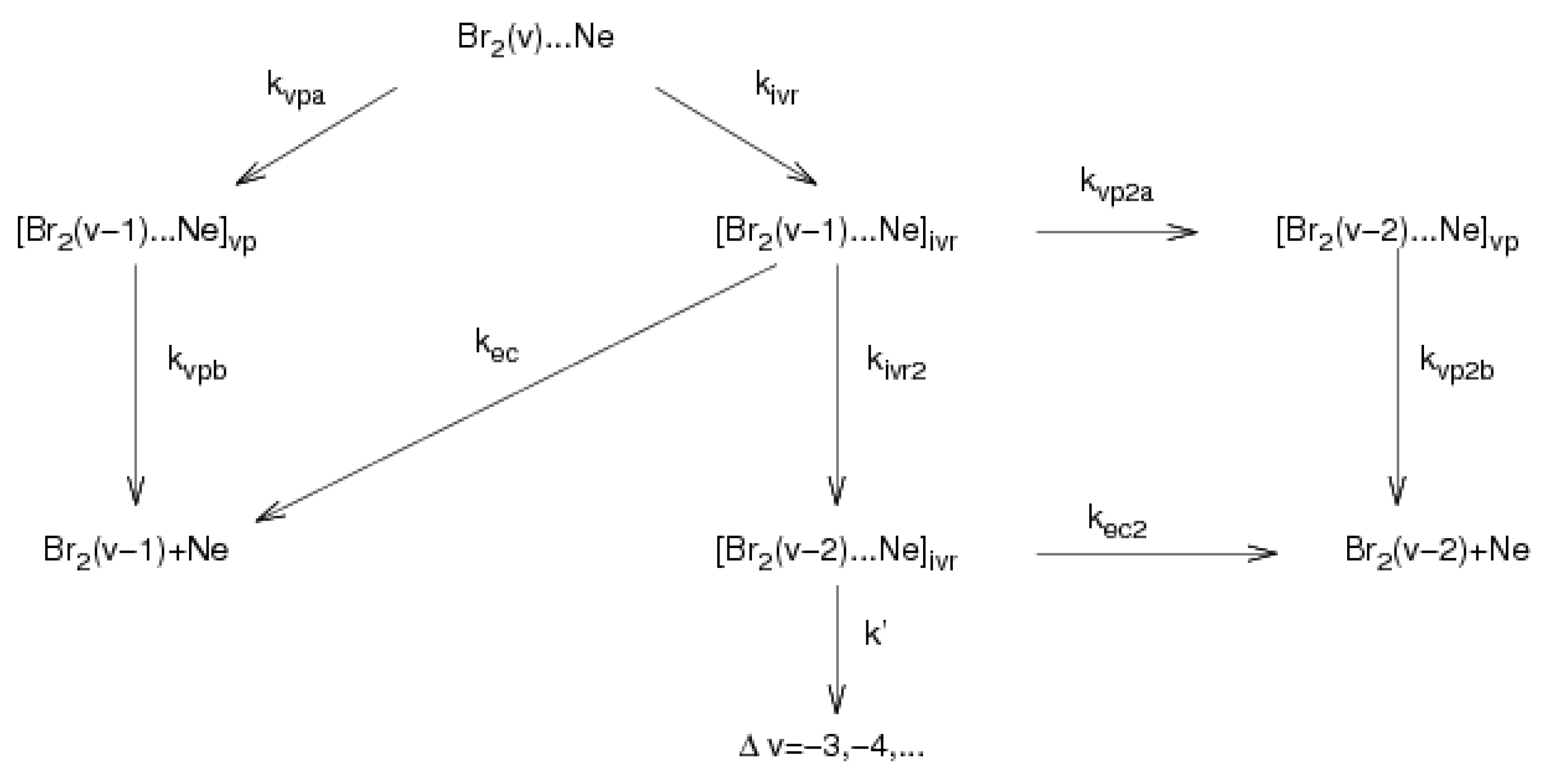
2.3. Kinetic Mechanism

The kinetic mechanism allows us to understand the path followed by our system as it relaxes and dissociates (see Figure 3). We consider Br 2 ( v i ) N e (intermediate state detected in the TSH simulation) as a sum of two contributions: a short-lived contribution coming from the VP process, which we denote by Br 2 ( v i ) Ne V P , and a longer-lived contribution coming from the IVR process denoted as Br 2 ( v i ) Ne I V R . Therefore, only the sum is taken into account to fit the kinetic rate constants. We include the Br 2 ( v i ) Ne V P intermediates in the direct VP process, dividing each direct VP step into two processes characterized by the rate constants k V P a and k V P b for the loss of the first vibrational quantum, and k V P 2 a and k V P 2 b for the loss of the second one.
We fit the data obtained in the simulation by using the next procedure:
[ Br 2 ( v ) Ne ] = [ { Br 2 ( v ) Ne } i v r + { Br 2 ( v ) Ne } v p ]
[ { Br 2 ( v ) Ne } i v r ] = k i v r k v e k v t
[ { Br 2 ( v ) Ne } v p ] = k v p a k v e k v t
[ Br 2 ( v 1 ) Ne ] = [ { Br 2 ( v 1 ) Ne } i v r + { Br 2 ( v 1 ) Ne } v p ]
[ { Br 2 ( v 1 ) Ne } i v r ] = k i v r k 1 k v ( e k v t e k 1 t )
[ { Br 2 ( v 1 ) Ne } v p ] = k v p a k v k v p b ( e k v p b t e k v t )
[ Br 2 ( v 1 ) ] = [ { Br 2 ( v 1 ) } i v r + { Br 2 ( v 1 ) } v p ]
[ { B r 2 ( v 1 ) } i v r ] = k i v r k e c ( k 1 k v ) k 1 k v k 1 ( 1 e k v t ) k v ( 1 e k 1 t )
[ { B r 2 ( v 1 ) } v p ] = k v p a ( k v k v p b ) k v k v ( 1 e k v p b t ) k v p b ( 1 e k v t )
[ Br 2 ( v 2 ) Ne ] = [ { Br 2 ( v 2 ) Ne } i v r + { Br 2 ( v 2 ) Ne } v p ]
[ { B r 2 ( v 2 ) N e } i v r ] = k i v r k i v r 2 ( k 1 k v ) ( k 2 k 1 ) ( k 2 k v ) { ( k 2 k 1 ) e k 1 t + + ( k v k 2 ) e k 1 t + ( k 1 k v ) e k 2 t }
[ { B r 2 ( v 2 ) N e } v p ] = k i v r k v p 2 a ( k 1 k v ) ( k 1 k v p 2 b ) ( k v p 2 b k v ) { ( k 1 k v p 2 b ) e k v t + + ( k v p 2 b k v ) e k 1 t + ( k v k 1 ) e k v p 2 b t }
[ Br 2 ( v 2 ) ] = [ { Br 2 ( v 2 ) } i v r + { Br 2 ( v 2 ) } v p ]
[ { B r 2 ( v 2 ) } i v r ] = k i v r k i v r 2 k e c 2 ( k 1 k v ) ( k 2 k 1 ) ( k 2 k v ) ( k 1 k v k 2 ) { k 2 k 1 ( k 2 k 1 ) ( 1 e k v t ) + k v k 2 ( k v k 2 ) ( 1 e k 1 t ) + k 1 k v ( k 1 k v ) ( 1 e k 2 t ) }
[ { B r 2 ( v 2 ) } v p ] = k i v r k v p 2 a ( k 1 k v ) ( k 1 k v p 2 b ) ( k v p 2 b k v ) ( k 1 k v ) { k 1 k v p 2 b ( k 1 k v p 2 b ) ( 1 e k v t ) + k v p 2 b k v ( k v p 2 b k v ) ( 1 e k 1 t ) + k v k 1 ( k v k 1 ) ( 1 e k v p 2 b t ) }
where:
  • k v = k v p a + k i v r
  • k 1 = k v p 2 a + k i v r 2 + k e c
  • k 2 = k e c 2 + k

2.4. Computational Details

In the methodology involved, two important stages contribute:
  • First stage
This step consists of propagating the dynamics of the system by evolving classically the nuclear motion on the potential energy surface. For this, employ the Adams Bashfort method [25], initiating with the method of Runge Kutta 4th order. We obtain, from the system of Equations (10)–(13), the momentum and coordinate of the Ne, the θ angle and the angular momentum of the system in Jacobi coordinates (see Figure 1). These coordinates are defined as follows: r is the distance between the diatomic constituents, R is the distance of the noble gas to the mass of the chemical bound and θ is the angle between r and R. In the method, some physical considerations of importance are imposed for obtaining a consistent result, such as the conservation of total energy. We consider that our system is dissociated beyond a certain maximum distance. For this, we take R m a x = 10 Å and a maximum time which the system will remain bounded, t m a x = 600 ps. Taking into account the above, we use an integration step equal to 0.1 ps, which leads to 6 × 10 6 integration cycles and ensuring a total energy conservation error of less than 10 8 cm 1 .
Simultaneously, in the other simulation thread, the Equation (20) is integrated, obtaining the c v coefficients. The c v c v * coefficients are the weight of each vibrational level (if v = v ) during the dynamics of the system and c v c v * (if v v ) indicate the coherence between states.
In order to apply the population conservation, the sum of the populations has to be equal the unity. We also incorporate a method for the hop decision (it is known as the Fewest Switches algorithm, see Appendix A). Another important aspect is the rescaling of the momentum to preserve the total energy of the system when the hop occurs.
To obtain the average interaction potentials of van der Waals, the Bode method is implemented. It is very important to define the average potentials and crossings between curves (see Figure 2).
  • Second stage
This stage consists of performing a fitting to initial, intermediate and final populations during the simulation. The complexity of doing this is that the parameters are shared and therefore obtaining these depends on the statistical behavior for each initial vibrational level. We followed the steps from the reference [29], which is a generalization of the Marquardt method for multiple equations and shared parameters.

3. Results and Discussion

The first two columns of Table 1 report the rate constants obtained by fitting the kinetic model to the TSH results for lifetimes and intermediate state dynamics (see Equation (31a)) using
τ = 1 k i v r + k v p a
Table 1 shows the rate constants obtained from the fitting of the TSH results to the kinetic mechanism. From this table we get much information about the path followed and the time spent in each initial, intermediate and final state. If ( k v p a > k v p b ) or ( k v p 2 a > k v p 2 b ), the system remains more time in the intermediate state before the dissociation occurs. However, if ( k v p b > k v p a ) or ( k v p 2 b > k v p 2 a ) occurs, the complex breaks its bond faster than otherwise. Moreover, for the lower vibrational levels, we obtained larger values for k v p b . This means that just after hopping, the molecule is dissociated. On the other hand, for the higher vibrational level there is a great probability of following an IVR process ( k i v r > k v p a ), and the others follow a VP process ( k v p a > k i v r ) . In addition, there is a competition between k e c and k i v r 2 . When k e c > k i v r 2 , the system is dissociated, losing a vibrational quantum number. In another case, the system is submitted to an IVR process again. In Figure 4, we show the lifetimes obtained.
In Figure 5, we show the process which the system followed until its dissociation.
In Figure 5, we can see that from vibrational level v = 21 the loss of two quanta through the VP v 0 2 process is significant. This causes the system to take longer to dissociate. Particularly for vibrational levels v = 28 , 29 , the predominant process is IVR-EC v 0 2 .
Through the simulation, we can know at what vibrational level the system is, and we do not need algorithms to obtain it. This is very good because the TSH method itself gives us that information. In the following figure, we present the exit channel (statistically) for each initial vibrational level.
As we can see in Figure 6 that the TSH results are in agreement with previous theoretical and experimental results. Other very important observables are E r o t and j m a x . The first one is the averaged rotational energy. The second one is the Br-Br angular momentum. Both quantities are calculated when the molecule is dissociated.
As we can appreciate in Figure 7, we report our results in comparison with experimental ones and previous results.
In Figure 8, we represent the rotational distributions of Br 2 after dissociation. We can see that there is a peak in the range of j = 20–24 (Figure 8c). This is an effect that we can see from v 0 = 21 to v 0 = 26, with the loss of two vibrational quantum numbers. This means that, for these vibrational levels having greater rotational excitation, the system takes a longer time to dissociate. Therefore, it does not have enough energy to break the vdW bond. They are non-reactive van der Waals modes and, as a direct consequence, the lifetimes are longer.
To analyze the conservation relation, we compute the correlation matrix for all vibrational levels under study. As we discussed before for the lowest vibrational levels ( v = 16–20), the fragmentation process occurs when the system loses one quantum energy. For those vibrational levels, more correlation is found for the k v p a and k i v r parameters. As we have shown in Figure 9, the parameter k e c shows a strong correlation with those parameters where the process involves two losses of quantum energy. Then, k e c plays an important role because it links the number of quantum energy losses in the fragmentation of the system ( Δ v = 1 , 2 , 3 . . . ).

4. Conclusions

We have investigated the vibrational predissociation process for the NeBr 2 system by using TSH method. In our simulation, we studied a range of vibrational levels (from v = 16 to v = 29 ). We found that the larger values for k v p b correspond to the lower vibrational levels. This is in correspondence with the dissociated of the molecule occurs just after hopping surface. As we comment in Section 3, there is a competition between VP and IVR processes. The TSH method is a robust methodology for the study of molecular fragmentation for this kind of system. This affirmation could be justified through Figure 6, Figure 7 and Figure 8. In these figures, we showed our results in comparison with the previous theoretical results and the experimental ones. As we can appreciate, the agreements are very good.

Perspectives

This method is a powerful tool for dealing with this type of system and can be extended to more complex structures (e.g., more vdW interactions). We continue with this work and we are checking that the strongest coupling belongs to v ± 1 . In that case, we must consider fewer surfaces for dynamics than before.

Author Contributions

These authors contributed equally to this work. Conceptualization, E.G.-A., M.M.-M., J.R.-S., N.H., K.C.J. and C.C.M.; Formal analysis, E.G.-A., M.M.-M., J.R.-S., N.H., K.C.J. and C.C.M.; Investigation, E.G.-A., M.M.-M., J.R.-S., N.H., K.C.J. and C.C.M.; Writing—review & editing, E.G.-A., M.M.-M., J.R.-S., N.H., K.C.J. and C.C.M. All authors have read and agreed to the published version of the manuscript.

Funding

This research received no external funding.

Acknowledgments

C.C.M. acknowledges support by the US National Science Foundation under CHE-1764209. This work is supported by the Programa Nacional de Ciencias Básicas de Cuba under Grant No. P223LH001-108 (E.G.-A., M.M.-M. and J.R.-S.).

Conflicts of Interest

The authors declare no conflict of interest.

Appendix A

We suppose that we have a quasiclassical system where the vibrational population for each state in the time t are determines for diagonal elements of ρ v v . For an ensemble of N trajectories that propagate simultaneously, the number of trajectories in the state v will be:
N v ( t ) = ρ v v ( t ) N
In t + Δ t the ocupation state will change to:
N v ( t + Δ t ) = ρ v v ( t + Δ t ) N
Assuming that N v ( t ) > N v ( t + Δ t ) , the minimum number of transitions neccessary for this change of occupation will be: N v ( t ) N v ( t + Δ t ) , hops from state | v to another ones, and 0 hops from any state to | v
The hopping probability out from state | v is:
P v ( t , Δ t ) = N v ( t ) N v ( t + Δ t ) N v ( t ) = ρ v v ( t ) ρ v v ( t + Δ t ) ρ v v ( t ) = Δ t ρ ˙ v v ( t ) ρ v v ( t ) Δ t ρ ˙ v v ( t ) ρ v v ( t )
where ( v v ) y ρ v v is the state where is has growing the population,
ρ ˙ v v ( t ) = c v ( t ) c v * ( t ) ˙ = c ˙ v * ( t ) c v ( t ) + c v * ( t ) c ˙ v ( t ) = ( c v * ( t ) c ˙ v ( t ) ) * + c v * ( t ) c ˙ v ( t ) = 2 R e ( c v * ( t ) c ˙ v ( t ) )
Replacing the last expression for (A3), we get:
P v = 2 R e ( c v * ( t ) c ˙ v ( t ) ) c v ( t ) c v * ( t ) .
Taking into account (20) and R e ( i c v ( t ) c v * ( t ) ) = I m ( c v ( t ) c v * ( t ) )
P v ( t ) = 2 Δ t v I m c v * ( t ) c v ( t ) e [ i ( E v E v ) t / ] v | H i n t ( r , R , θ ) | v c v ( t ) c v * ( t ) = v v P v v
Changing the notation then gives
g v ( t ) = v v g v v ( t )
g v v ( t ) = m a x 0 , 2 Δ t I m c v * ( t ) c v ( t ) e [ i ( E v E v ) t / ] | c v ( t ) | 2 v | H i n t ( r , R , θ ) | v
  • if g v v < 0 , then g v v = 0 .
To determine whether a hop from the | v surface is realized, we chose a random number 0 < η < 1 . We use a uniform distribution.
  • if 0 < η < g v v , the system hops to surface | v . We considered ordered states ( v , v , v " , ) .
  • if g v v < η < g v v + g v v " , the system hops to surface | v " > .
  • if v v g v v < η < 1 , then system remains in state v.

References

  1. Wilberg, D.M.; Gutmann, M.; Breen, J.J.; Zewail, A.H. Real-time dynamics of clusters. I. I2 Xn (n = 1). J. Chem. Phys. 1992, 96, 198. [Google Scholar] [CrossRef] [Green Version]
  2. Gutmann, M.; Wilberg, D.M.; Zewail, A.H. Real-time dynamics of clusters. II. I2Xn, (n = 1; X = He, Ne, and H2), picosecond fragmentation. J. Chem. Phys. 1992, 97, 8037. [Google Scholar] [CrossRef] [Green Version]
  3. Borrell-Grueiro, O.; Márquez-Mijares, M.; Pajón-Suárez, P.; Hernández-Lamoneda, R.; Rubayo-Soneira, J. Fragmentation dynamics of NO–NO dimer: A quasiclassical dynamics study. Chem. Phys. Lett. 2013, 563, 20. [Google Scholar] [CrossRef]
  4. Rubayo-Soneira, J.; Garcıía-Vela, A.; Delgado-Barrio, G.; Villarreal, P. Vibrational predissociation of I2-Ne. A quasiclassical dynamical study. Chem. Phys. Lett. 1995, 243, 236. [Google Scholar]
  5. García-Vela, A.; Rubayo-Soneira, J.; Delgado-Barrio, G.; Villarreal, P. Quasiclassical dynamics of the I2–Ne2 vibrational predissociation: A comparison with experiment. J. Chem. Phys. 1996, 104, 8405. [Google Scholar] [CrossRef] [Green Version]
  6. Roncero, O.; Campos-Martıínez, J.; Hernández, M.I.; Delgado-Barrio, G.; Villarreal, P.; Rubayo-Soneira, J. Photodissociation of NeBr2(B) below and above the dissociation limit of Br2(B). J. Chem. Phys. 2001, 115, 2566. [Google Scholar] [CrossRef] [Green Version]
  7. Cabrera, J.A.; Bieler, C.R.; Olbricht, B.C.; Veer, W.E.v.; Janda, K.C. Time-dependent pump-probe spectra of NeBr2. J. Chem. Phys. 2005, 123, 054311. [Google Scholar] [CrossRef]
  8. González-Martínez, M.L.; Rubayo-Soneira, J.; Janda, K. Quasi-classical trajectories study of Ne79Br2(B) vibrational predissociation. Phys. Chem. Chem. Phys. 2006, 8, 4550. [Google Scholar] [CrossRef]
  9. García-Vela, A.; Janda, K.C. Quantum dynamics of Ne-Br2 vibrational predissociation: The role of continuum resonances and doorway states. J. Chem. Phys. 2006, 124, 034305. [Google Scholar] [CrossRef]
  10. Cline, J.I.; Evard, D.D.; Reid, B.P.; Sivakumar, N.; Thommen, F.; Janda, K.C. Structure and Dynamics of Weakly Bound Molecular Complexes; Weber, A., Ed.; Reidel: Dordrecht, The Netherlands, 1987; pp. 533–551. [Google Scholar]
  11. González-Martínez, M.L.; Arbelo-González, W.; Rubayo-Soneira, J.; Bonnet, L.; Rayez, J.-C. Vibrational predissociation of van der Waals complexes: Quasi-classical results with Gaussian-weighted trajectories. Chem. Phys. Lett. 2008, 463, 65. [Google Scholar] [CrossRef]
  12. Reed, S.K.; González-Martínez, M.L.; Rubayo-Soneira, J.; Shalashilin, D.V. Cartesian coupled coherence states simulations: NenBr2 dissociation as a test case. J. Chem. Phys. 2011, 134, 054110. [Google Scholar] [CrossRef]
  13. Borrell-Grueiro, O.; Baños-Rodrıíguez, U.; Márquez-Mijares, M.; Rubayo-Soneira, J. Vibrational predissociation dynamics of the nitric oxide dimer. Eur. Phys. J. D 2018, 72, 121. [Google Scholar] [CrossRef]
  14. Prosmiti, R.; Cunha, C.; Buchachenko, A.A.; Delgado-Barrio, G.; Villarreal, P. Vibrational predissociation of NeBr2(X, v=1) using an ab initio potential energy surface. J. Chem. Phys. 2002, 117, 22. [Google Scholar] [CrossRef] [Green Version]
  15. Miguel, B.; Bastida, A.; Zúñiga, J.; Requena, A.; Halberstadt, N. Time evolution of reactants, intermediates, and products in the vibrational predissociation of Br2⋯Ne: A theoretical study. J. Chem. Phys. 2000, 113, 22. [Google Scholar] [CrossRef]
  16. Stephenson, T.A.; Halberstadt, N. Quantum calculations on the vibrational predissociation of NeBr2: Evidence for continuum resonances. J. Chem. Phys. 2000, 112, 5. [Google Scholar] [CrossRef] [Green Version]
  17. Tully, J.C. Molecular dynamics with electronic transitions. J. Chem. Phys. 1990, 93, 1061. [Google Scholar] [CrossRef]
  18. Rodríguez–Fernández, A.; Márquez-Mijares, M.; Rubayo-Soneira, J.; Zanchet, A.; García-Vela, A.; Bañares, L. Trajectory surface hopping study of the photodissociation dynamics of methyl radical from the 3s and 3pz Rydberg states. Chem. Phys. Lett. 2018, 712, 171–176. [Google Scholar] [CrossRef]
  19. Rodríguez–Fernández, A.; Márquez–Mijares, M.; Rubayo–Soneira, J.; Zanchet, A.; Bañares, L. Quasi-classical study of the photodissociation dynamics of the methyl radical. Rev. Cuba. Fis. 2017, 34, 41. [Google Scholar]
  20. Martens, C.C. Communication: Fully coherent quantum state hopping. J. Chem. Phys. 2015, 143, 141101. [Google Scholar] [CrossRef] [Green Version]
  21. Bastida, A.; Zúñiga, J.; Requena, A.; Halberstadt, N.; Beswick, J.A. Competition between electronic and vibrational predissociation in Ar–I2 (B): A molecular dynamics with quantum transitions study. Chem. Phys. 1999, 240, 229–239. [Google Scholar] [CrossRef]
  22. Nangia, S.; Jasper, A.W.; Miller, T.F., III; Truhlar, D.G. Army ants algorithm for rare event sampling of delocalized nonadiabatic transitions by trajectory surface hopping and the estimation of sampling errors by the bootstrap method. J. Chem. Phys. 2004, 120, 3586. [Google Scholar] [CrossRef] [Green Version]
  23. Subotnik, J.E.; Ouyang, W.; Landry, B.R. Can we derive Tully’s surface-hopping algorithm from the semiclassical quantum Liouville equation? Almost, but only with decoherence. J. Chem. Phys. 2013, 139, 214107. [Google Scholar] [CrossRef] [Green Version]
  24. Buchachenko, A.A.; Baisogolov, A.Y.; Stepanov, N.F. Interaction Potentials and Fragmentation Dynamics of the Ne-Br2 Complex in the Ground and Electronically Excited States. J. Chem. Soc. Faraday Trans. 1994, 90, 3229–3236. [Google Scholar] [CrossRef]
  25. Burden, R.L.; Faires, J.D. Numerical Analysis, 9th ed.; Julet, M., Ed.; Brooks/Cole Cengage Learning: Boston, MA, USA, 2010; pp. 173–259. [Google Scholar]
  26. Crespo-Otero, R.; Barbatti, M. Recent advances and perspectives on nonadiabatic mixed quantum-classical dynamics. Chem. Rev. Am. Chem. Soc. 2018, 118, 15. [Google Scholar] [CrossRef] [Green Version]
  27. Requena, A.; Halberstadt, N.; Beswick, J.A.; Sola, I.; Bastida, A.; Zúñiga, J. Application of trajectory surface hopping to vibrational predissociation. Chem. Phys. Lett. 1997, 280, 185–187. [Google Scholar]
  28. Jasper, A.W.; Truhlar, D.G. Improved treatment of momentum at classically forbidden electronic transitions in trajectory surface hopping calculations. Chem. Phys. Lett. 2003, 369, 60–67. [Google Scholar] [CrossRef]
  29. Spitzer, P.; Zierhofer, C.; Hochmair, E. Algorithm for multicurve-fitting with shared parameters and a possible application in evoked compound action potential measurements. Biomed. Eng. Online 2006, 5, 13. [Google Scholar] [CrossRef] [Green Version]
  30. Nejad-Sattari, M.; Stephenson, T.A. Fragment rotational distributions from the dissociation of NeBr2: Experimental and classical trajectory studies. J. Chem. Phys. 1997, 1016, 5454. [Google Scholar] [CrossRef] [Green Version]
Figure 1. Jacobi coordinates for NeBr 2 molecule.
Mathematics 08 02029 g001
Figure 2. Schematic figure of the van der Waals interaction. The curves are calculated for the “T” shaped configuration ( θ = 90 ).
Mathematics 08 02029 g002
Figure 3. Scheme of kinetic mechanism.
Mathematics 08 02029 g003
Figure 4. Lifetime for different initial vibrational level of Br 2 .
Mathematics 08 02029 g004
Figure 5. Path followed (statistically) for each vibrational level.
Mathematics 08 02029 g005
Figure 6. Exit channel.
Mathematics 08 02029 g006
Figure 7. Average rotational energy [ E r o t cm 1 ] and the maximum orbital angular momentum ( j m a x ) (see reference [8] to compute j m a x ).
Mathematics 08 02029 g007
Figure 8. Rotational distribution for the transitions (a) v = 21–20, (b) v = 22–21, (c) v = 24–22, (d) v = 29–27. Experimental results correspond to [30].
Mathematics 08 02029 g008
Figure 9. Correlation matrix for vibrational level v = 23 .
Mathematics 08 02029 g009
Table 1. Rate constants (in n s 1 ) obtained by fitting the trajectory surface hopping (TSH) simulation results.
v 0 k ivr k vpa k v k 1 k vpb k ec k ivr 2 k 2 k vp 2 b k ec 2 k vp 2 a
160.0244.4564.60081,0198,050,0001,704,73051,9482,523,430604.148361.25824,245
170.1105.7165.88760,896882.070733.63415,961846.233150.9621948153,785
180.0555.4105.62020,1242935.5771328,970818.53512.646333523,207
191.48412.80513.99163,190223.312190715,356217.080499.413496.26311,185
202.74214.91416.97055,278185734.1477684171.37918.734769.6981929
2111.99935.60841.822475162.68414.016211.989123.330169.610197.089791.290
223.93414.95618.8215723228.02026.9789367.42539.847932.066145.8673575
234.68516.54020.9965263168.90429.0351023118.771268.294102.7443339
243.96613.34517.937138.804237.4821.030157.18019114412551.14186.110
2510.39719.05529.327149.336142.79412.052132.47218211507261.61986.482
2611.93716.68629.887100.351126.8200.157118.667350265011001.19048.893
27115.1500.153105.52076.8820.11025.24950.9491826692,71834.39132.183
2869.2952.47871.94085.52512502.920160412,15216,751444.0405.350
29133.7503.642127.64081.4607.2872.087153612,27611,827431.9415.684
Publisher’s Note: MDPI stays neutral with regard to jurisdictional claims in published maps and institutional affiliations.

