Trends in Super-High-Definition Imaging Techniques Based on Deep Neural Networks

Abstract

Images captured by cameras in closed-circuit televisions and black boxes in cities have low or poor quality owing to lens distortion and optical blur. Moreover, actual images acquired through imaging sensors of cameras such as charge-coupled devices and complementary metal-oxide-semiconductors generally include noise with spatial-variant characteristics that follow Poisson distributions. If compression is directly applied to an image with such spatial-variant sensor noises at the transmitting end, complex and difficult noises called compressed Poisson noises occur at the receiving end. The super-high-definition imaging technology based on deep neural networks improves the image resolution as well as effectively removes the undesired compressed Poisson noises that may occur during real image acquisition and compression as well as in transmission and reception systems. This solution of using deep neural networks at the receiving end to solve the image degradation problem can be used in the intelligent image analysis platform that performs accurate image processing and analysis using high-definition images obtained from various camera sources such as closed-circuit televisions and black boxes. In this review article, we investigate the current state-of-the-art super-high-definition imaging techniques in terms of image denoising for removing the compressed Poisson noises as well as super-resolution based on the deep neural networks.

1. Introduction

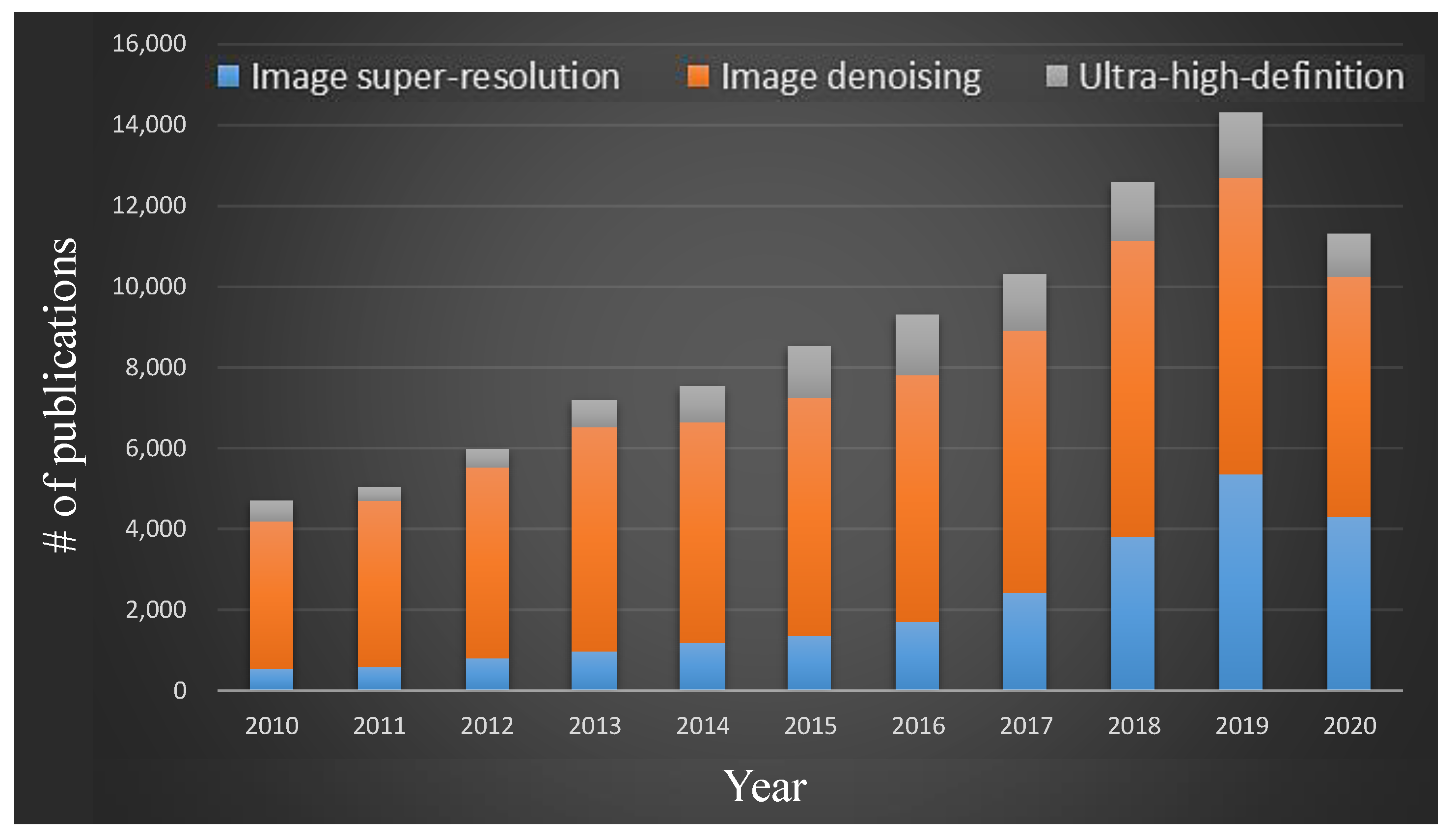
This review article is based on super-high-definition image generation methods and introduces deep neural networks (DNN) that convert noisy low-resolution images into clean high-resolution images. Figure 1 shows the number of published papers on image super-resolution, image denoising, and ultra-high-definition. The values in the figure were obtained through the keyword search on the Google Scholar website. The number of publications in 2020 is expected to continue to increase by the end of this year. In Figure 1, on average, about 12,730 papers dealing with three keywords have been published annually over the last three years, and this trend of the chart shows the popularity of the research topic covered in this review article.

Usually, unwanted noises are present in the images captured by any camera. Particularly, images captured in dark environments show deterioration owing to noise. Several filters for removing the noise from the images have been developed. For example, a certain noise removal method calculates the weighted average of neighboring pixel values using a Gaussian filter [1]. However, this method flattens the edge regions while generating clear high-quality images by removing noises. To compensate for this limitation, several filters have been devised to improve the image quality for both the flat and edge regions with low computational complexity—the bilateral filter is the representative filter [2]. However, the bilateral filter that is mainly proposed to remove the well-known ringing or blocking artifacts has a limitation in removing compressed Poisson noises generated during the compression of noisy images. Consequently, a method to more accurately reconstruct a high-resolution image by removing the compressed Poisson noises in the image is required. In this section, we introduce DNN-based denoising techniques [3,4] to remove the compressed Poisson noises and DNN-based super-resolution techniques to convert low-resolution images into high-resolution images.

A typical imaging system comprises image acquisition, transmission, and reception, as shown in Figure 2.

In the figure, let z be a decoded block in the receiver as

$$z(x)=T^{-1}\left\{round\left\{\frac{T\left\{aP(x)\right\}}{Q}\right\}\times Q\right\}$$

(1)

where x denotes a spatial coordinate, and T and T⁻¹ are block discrete cosine transform (BDCT) and inverse BDCT (IBDCT) operators, respectively. In addition, P denotes a Poisson variable scaled by a with a mean value μ, and Q denotes a quantization table. Here, the probability distribution of the acquired value P(x) is derived in [4,5] as

$$p(P(x)|\mu )=\frac{{\mu }^{P(x)}{e}^{-\mu }}{P(x)!}$$

(2)

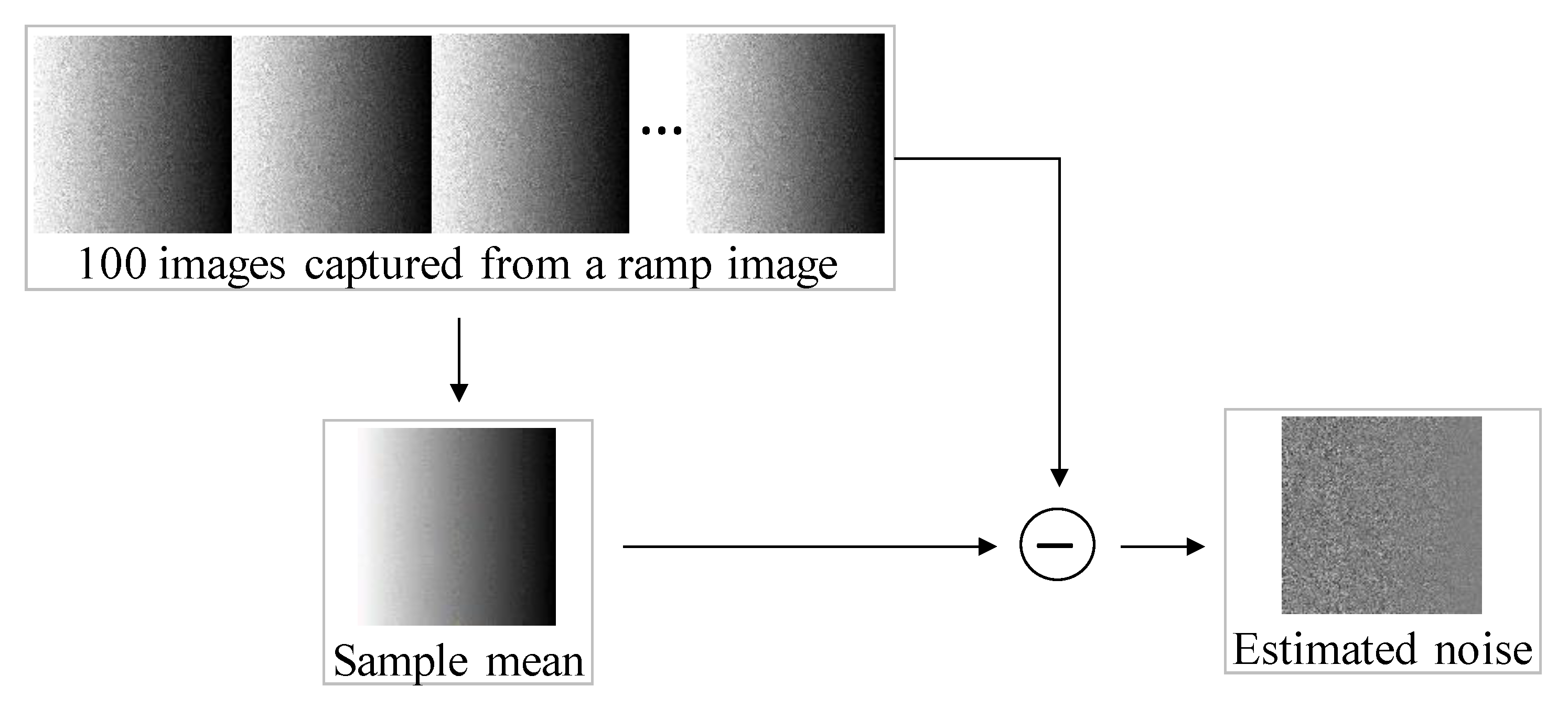
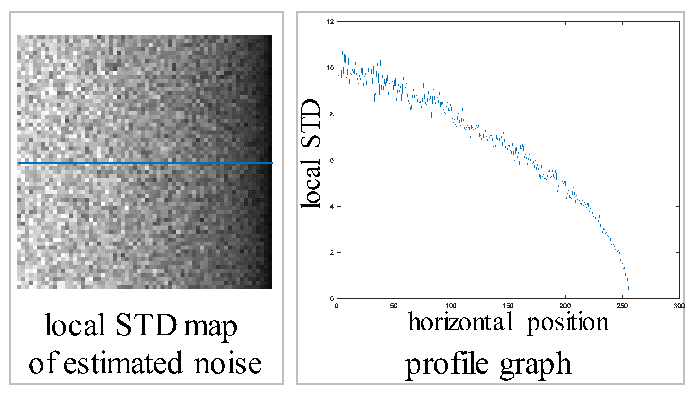
In the image acquisition stage, images are acquired through charge-coupled devices (CCDs) or complementary metal-oxide-semiconductor (CMOS) camera sensors. At this point, noise inevitably occurs in the image owing to the limitations of the camera sensor. In [3], to observe this sensor noise, a ramp image whose brightness gradually changes in the horizontal direction in a dark lighting environment was placed. Then, the image was captured 100 times using a fixed camera. To this end, the camera settings involved a short exposure time and high ISO value to facilitate noise observation. As illustrated in Figure 3, to check the noise characteristics, a clean sample mean image was obtained using the average of 100 images, and only the noise was extracted through the difference between 100 individual noisy images and the sample mean image. By calculating the local standard deviation of the extracted noise and checking the local standard deviation variation in the horizontal direction, it was confirmed that the standard deviation or variance of the noise has a spatial-variant characteristic that changes according to the position in the image, as shown in Figure 4. Given an image having Poisson noise with a spatial-variant characteristic, the following operations are performed: (i) encoding during the image transmission stage using discrete cosine transformation (DCT) domain quantization and (ii) inverse quantization during the reception stage. As shown in Figure 2, in addition to well-known noises such as blocking and ringing artifacts, compressed Poisson noise in the form of random dots is also generated. In the same figure, the residual image obtained through the difference between the original ground truth (GT) image and the decoded image shows complex-pattern noise even in the flat region that had no signal. According to [4], the complex pattern deformed by compression is called compressed Poisson noise. It is considered that an accurate image degradation model and a robust image reconstruction technique for spatial-variant noise characteristics are additionally required for removing the compressed Poisson noise.

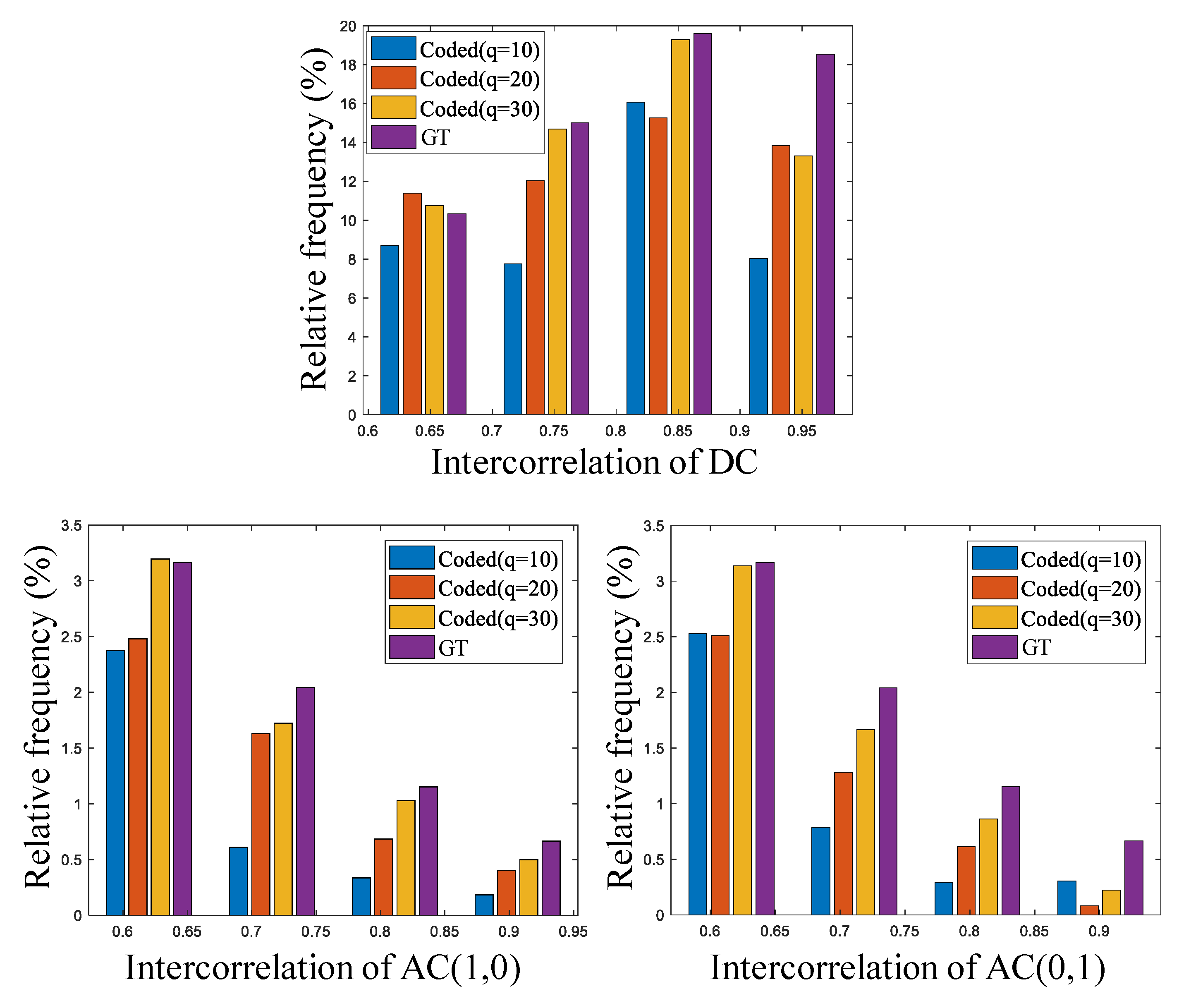
Additionally, in [4], to observe the inter-block correlation distortion of an image owing to block-based compression, the original GT image is analyzed with various JPEG quality factors (q = 10, 20, and 30) corresponding to low transmission rates. While performing image compression at the compression level, the distribution of correlation values between the blocks was obtained, as shown in Figure 5. Here, it was observed that the smaller the value of q, the higher the compression level achieved. From the results, it was confirmed that the inter-block correlation value for low-frequency DCT coefficients decreases as the compression level increases. In this figure, three coefficients are used as examples. On the contrary, this tendency did not hold true for the correlation distribution for other high-frequency DCT coefficients. Consequently, it can be determined that a correlation enhancement method for low-frequency DCT coefficients is necessary to effectively reconstruct a low-rate block-based compressed image.

Based on the experiments presented in Figure 2, Figure 3, Figure 4 and Figure 5, the compressed Poisson noise reduction technique in the secondary domain was proposed [4]. Here, the secondary block domain was proposed to enhance inter-block correlation, and the variance-stabilized neural network was proposed to cope with the spatial-variant noise characteristics.

Furthermore, information about patch direction proves to be very useful for accurate image restoration such as super-resolution imaging because it can be an important clue in recovering high-frequency components that are lost owing to image downscaling and compression. Typically, DNN-based super-resolution techniques tend to maintain the robustness of the super-resolution performance in any direction of the input low-resolution patch by utilizing a public training dataset comprising image patches with various directions [6,7,8,9]. Contrary to this trend, it is noted that the method can improve the clarity of the input low-resolution patch for a specific direction while training a neural network model based on a patch dataset with a specific direction. Moreover, by retraining the model parameters of the existing super-resolution technique based on the convolutional neural network (CNN) for each direction (0 to 180°), it is possible to achieve super-resolution performance comparable to that expected in [10]. However, storing a large number of models in all patch directions not only requires a huge amount of memory but also involves considerable computational complexity in the training process. To alleviate this problem, a patch-orientation-specified network (POSNet) is developed in [10] by constructing a dataset with a specific direction and an angle transformation in the same direction as the constructed dataset is applied to the input patch. Additionally, a new patch orientation-specified neural network system is proposed by combining this angle conversion technique with a DNN specially designed for super-resolution. Furthermore, a non-specified neural network for maintaining super-resolution performance is proposed for patches with multiple directions, and the proposed two neural networks are adaptively applied according to the information about the input patch direction.

In this paper, we describe both image denoising and super-resolution imaging techniques based on DNN. Unlike in the existing review paper [11], note that this paper reviews compressed image denoising technologies as well as the latest state-of-the-art super-resolution ones. To this end, Section 2 describes the secondary-domain variance-stabilized neural network for image denoising. Section 3 describes several DNNs for super-resolution imaging. The quantitative performance comparison is presented in Section 4, and finally, Section 5 states the conclusion.

2. DNN Model for Compressed Poisson Noise Reduction

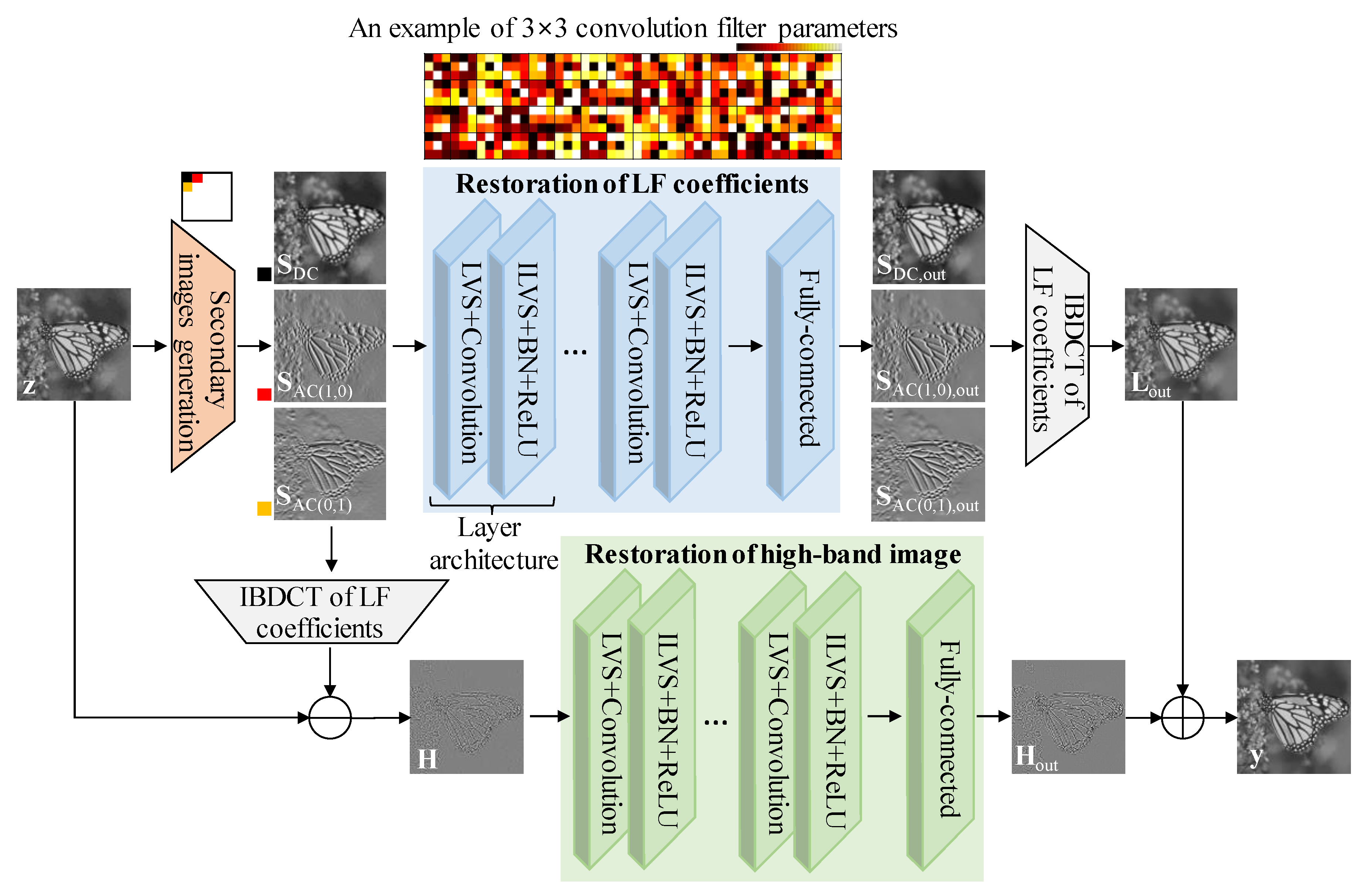
Among several image denoising areas such as reductions of Gaussian noises [12,13,14,15], Poisson noises [3,5,16,17], Poisso-Gaussian noises [18,19,20,21], impulse noises [22,23,24,25], compressed noises [26,27,28,29,30,31], and compressed Poisson noises, this section introduces compressed Poisson noise reduction that the researchers may not find familiar, but it is very important for achieving super-high-definition imaging. The concept of the compressed Poisson noise was first introduced in 2019 in [4], and the architecture of the compressed Poisson noise reduction technique [4] is illustrated in Figure 6. It comprises secondary image generation, restoration of low-frequency coefficients, IBDCT of low-frequency coefficients, and restoration of a high-band image.

The secondary image generation module calculates the low-frequency BDCT coefficient value by shifting a fixed-size block by one pixel for an input image. Subsequently, the coefficient values obtained from all blocks are aggregated into one image for each coefficient to obtain the secondary image. Accordingly, each secondary image has the same size as that of the input image, and the pixel value comprises low-frequency DCT coefficient values. The restoration of low-frequency coefficients removes noise and restores the image similar to the uncompressed original secondary image by enhancing the inter-block correlation within the compressed image. Specifically, the neural network for restoring low-frequency coefficients comprises the repetition of a layer architecture, and the layer architecture comprises variance stabilization transform (VST), convolution, inverse VST (IVST), batch normalization (BN), and rectified linear unit (ReLU). The secondary image received as the input of the neural network is adjusted such that the local variance value of the compressed Poisson noise is the same at all positions in the image through the VST as

$$f(s)=\{\begin{array}{l}2\sqrt{s+3/8} ,\hspace{1em}s\ge -3/8\\ \hspace{1em} \hspace{1em}0\hspace{1em} ,\hspace{1em} \mathrm{otherwise} \end{array}$$

(3)

where s denotes the secondary image pixel value.

To perform subsequent convolution, the convolution filter parameters were pre-trained to minimize the mean squared error (MSE) between the original secondary images and the corresponding neural network outputs. Here, the number of filters is set to 64, and the filter size is set to 3 × 3 in every layer architecture. The top of Figure 6 shows an example of convolution filter parameters that are obtained via the network training. The convolution is performed using these pre-trained parameters. Subsequently, it is returned to the original local variance value through the IVST, and the convergence speed in the learning process is increased by using the BN and ReLU. The layer architecture comprising these five detailed modules is repeated several times, and the output shape is returned to the input image size by passing one fully connected layer through the last output feature map result. The IBDCT of the low-frequency coefficients in the upper right corner of Figure 6 performs the IBDCT while outputting a low-band image when moving the block size so that blocks do not overlap by using the result of the low-frequency coefficient recovery unit. The IBDCT of the low-frequency coefficients located at the top right of Figure 6 receives the result of the low-frequency coefficient restoration as an input and generates an output low-band image by applying the IBDCT while moving the block without any overlap. In the high-band image restoration of Figure 6, the input high-band image is obtained through the difference between the input noisy image and its low-band image obtained previously. Next, the output high-band image is obtained by passing a neural network comprising repeated-layer architectures and the fully connected layer defined by the low-frequency coefficient restoration. To this end, the convolution filter parameters were pre-trained so that the MSE between the neural network’s output of the high-band image obtained from the compressed Poisson noisy image and the corresponding original high-band image is minimized. According to [4], the learning rate was set to drop exponentially from 0.001 to 0.00001, and the network was trained on one NVIDIA GTX 1080 GPU under MATLAB R2017b with the MatConvNet package for about 16 h. In addition, the whole inference time was about 120 ms for a 512 × 512 image.

3. DNN Model for Image Super-Resolution

3.1. Conventional Image Super-Resolution Models

In the image acquisition model, a high-resolution image x is warped at the camera lens with relative motion between the scene and camera, B_motion. The warped image is blurred by an imperfect camera lens with B_cam and then discretized to the CCD resolution with down-sampling operator D. By defining point spread function as B = B_camB_motion, we can represent the image acquisition model as follows:

y = DBx + n,

(4)

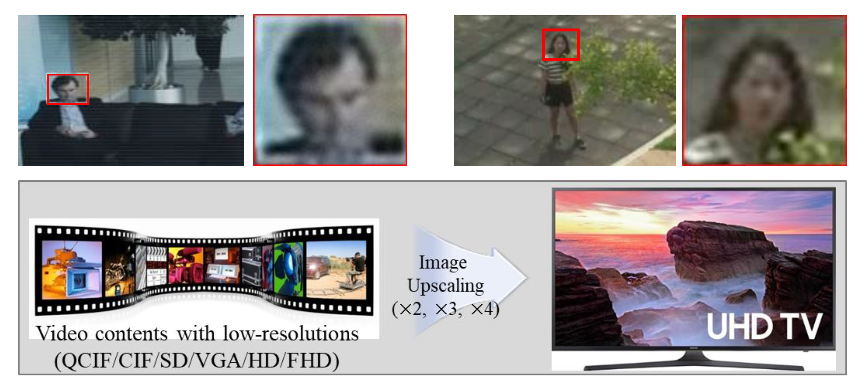
where y and n denote the acquired low-resolution image and the system noise, respectively. Single image super-resolution restores a high-resolution image x from a low-resolution one y. This restoration process is considered an ill-posed problem that cannot estimate the GT from the low-resolution image via regular inverse filtering. As shown in the first row of Figure 7, images captured by CCTVs and black box cameras tend to have low image quality owing to several reasons such as lens distortion, optical blur, resolution limitation, and low bit-rate compression. Therefore, image resolution enhancement or super-resolution is required to increase the accuracy in object recognition areas. Moreover, recent displays such as ultra-high-definition television (UHDTV) and light-emitting diode (LED) signage have improved display resolution. However, most of the existing video content has a low-resolution; therefore, highly accurate image upscaling techniques are required, as shown in the second row of Figure 7.

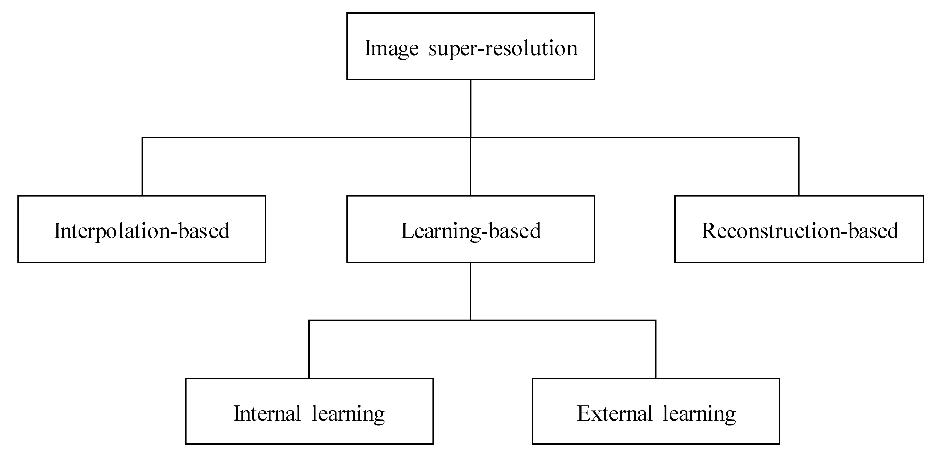
The approach for image super-resolution can be divided into three classes, as illustrated in Figure 8. The first comprises interpolation-based methods such as bilinear, bicubic, and Lanczos interpolations. Although interpolation-based methods are considerably fast, their resolution improvement effect is relatively low. The second comprises the reconstruction-based method using inverse optimization. This method requires a complex iterative optimization process instead of the training process. The third comprises learning-based methods such as patch matching, machine learning, CNN, and generative adversarial network. Among the aforementioned three super-resolution approaches, the learning-based method tends to provide the best visual performance. This method is divided into two classes: internal and external learning. However, in this learning-based method, a pre-training process is required, and the super-resolution performance is highly dependent on the training database.

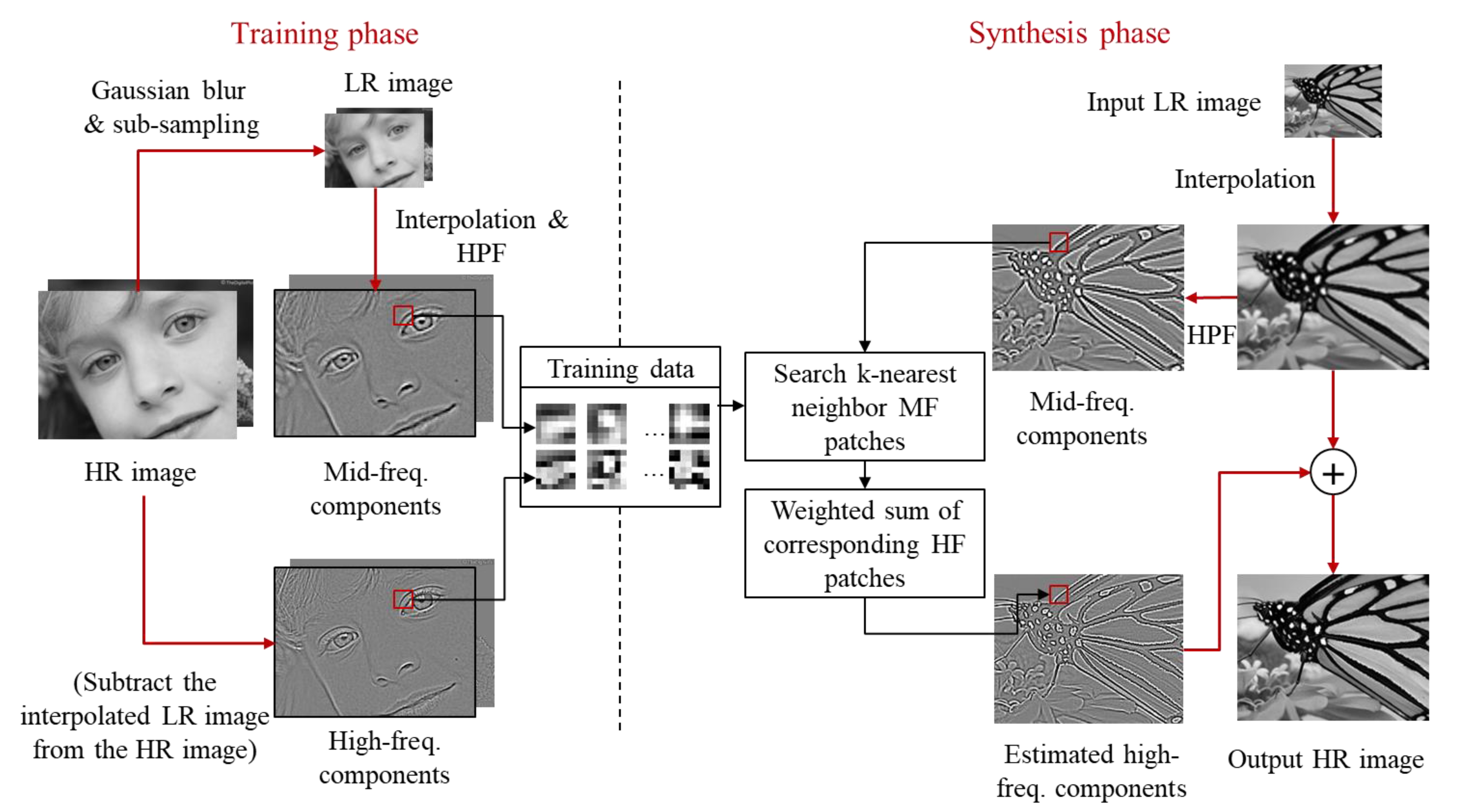
In this section, the learning-based super-resolution approach is mainly discussed, since it usually provides the best performance among three approaches. An example-based method using an external dictionary was first proposed in [6]. Herein, the paired data comprising high-resolution images and the corresponding low-resolution images were prepared for the training procedure, as shown in Figure 9. From the prepared data, the feature is first extracted from the training images and then saved to each dictionary. In the testing procedure, the same feature extraction is applied to each low-resolution patch, and feature matching is performed. Using the matched high-resolution feature, the output high-resolution image can be synthesized.

Another method [7] proposed the example-based super-resolution using external learning and structure analysis of patches, as shown in Figure 10. This method utilizes the sharpness of high-resolution patch candidates for the reliable determination of high-frequency patches. For each input patch, a sufficient number of high-frequency patches are preselected from a training database. Based on the reconstruction constraint in the low-resolution domain, the outlier high-frequency patches are removed. Finally, the method reselects several high-frequency patches according to patch characteristics to reproduce the final high-resolution image. After the high-frequency patch selection, a pixel-level optimization process based on robust statistics is performed.

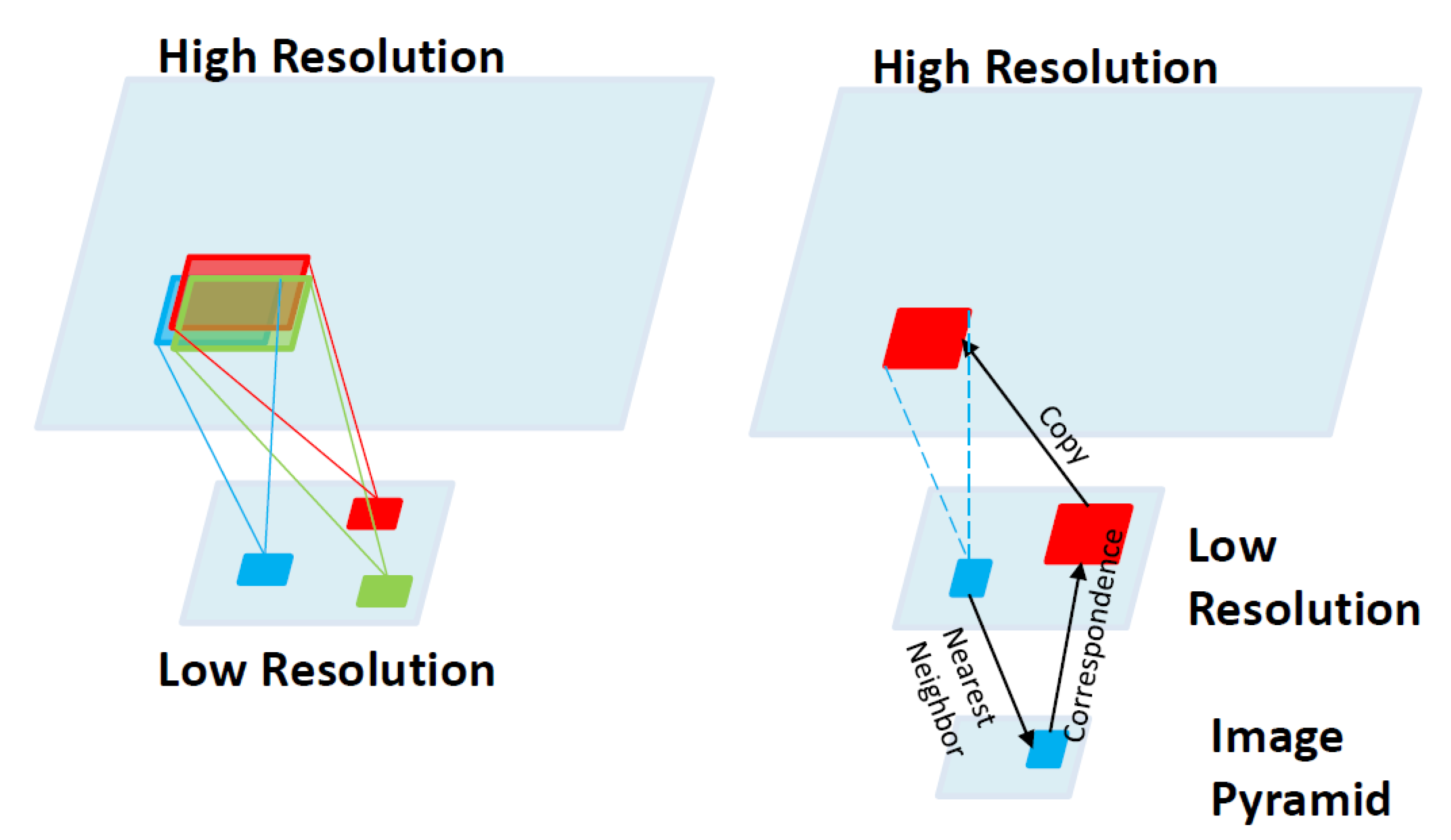
In another approach to learning-based super-resolution, a self-example-based method without an external database or prior examples was proposed [8]. This approach is based on the observation regarding patch redundancy both within the same scale and across different scales, as shown in Figure 11. In this figure, the left and right images show the in-scale and cross-scale patch redundancies, respectively. By combining example-based patch matching constraints with classical reconstruction constraints, a single unified super-resolution framework was developed.

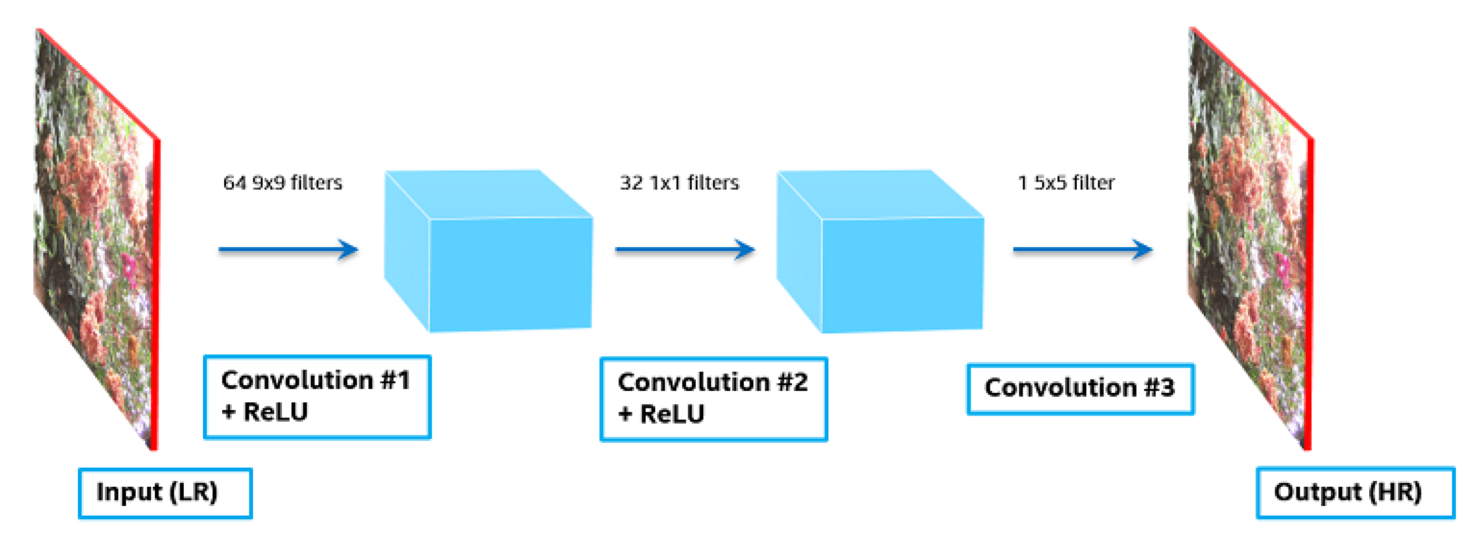
In [9], a deep learning method based on CNN was proposed for single-image super-resolution, as shown in Figure 12. Herein, the end-to-end mapping between the low and high-resolution images is represented as a deep CNN with a lightweight structure. For this, the first convolutional layer extracts a set of feature maps, and the second transforms these feature maps nonlinearly into high-resolution representations. The last layer combines the representations to produce the output high-resolution image. Generally, in the deep learning-based super-resolution approach, the convolutional layer located at the front side serves in extracting low-level features, and the convolutional layer located at the rear side serves to extract high-level features. The non-linear activation function such as ReLU enables the effective training of deep CNNs by reducing the gradient vanishing problem and the computation time. Consequently, the trained CNN architecture with multiple convolutional layers and non-linear activation functions plays a key role in solving the ill-posed super-resolution problem in (4) by exploiting both low-level features and high-level features.

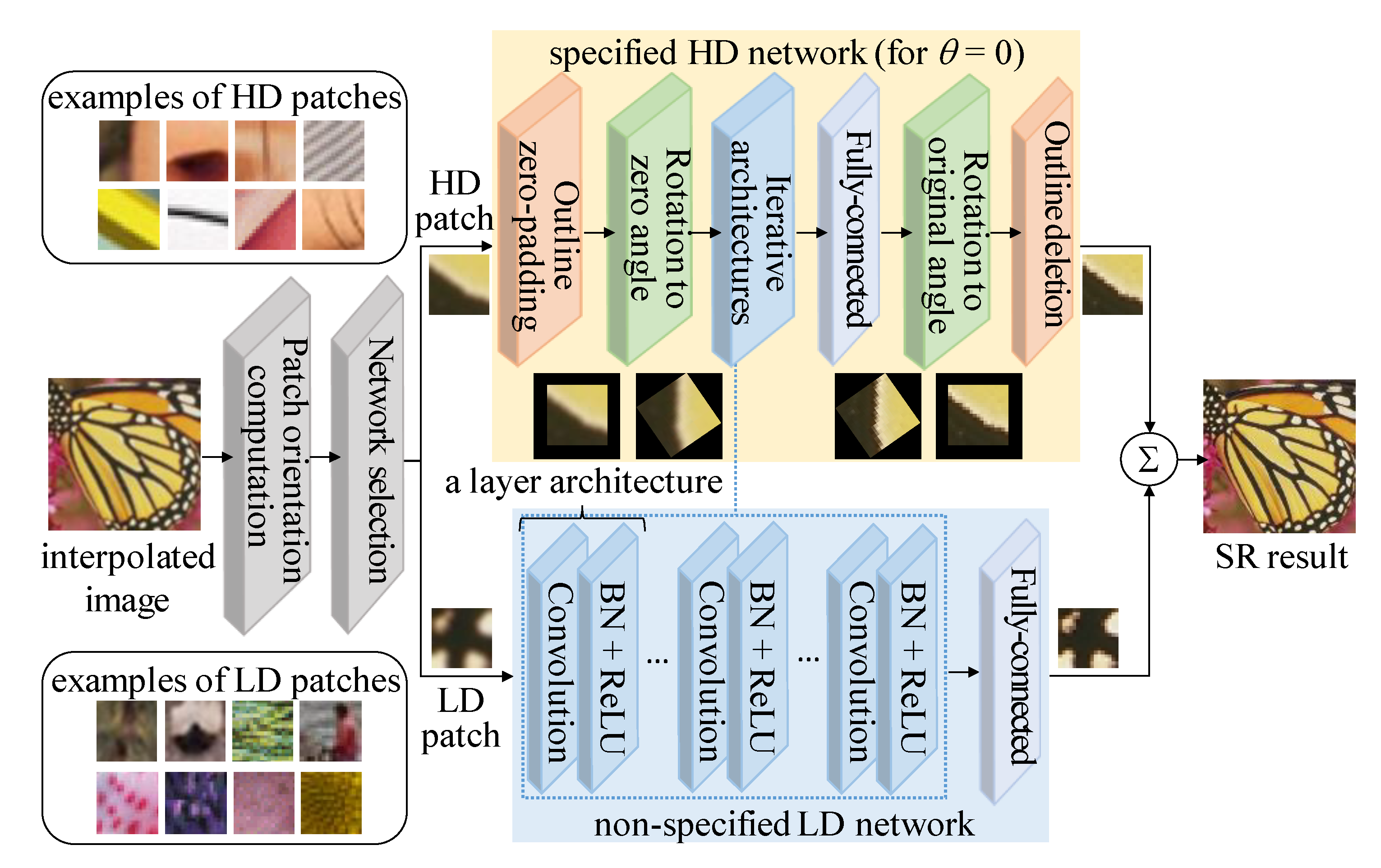
Moreover, to facilitate both unidirectional and multidirectional input patches in the technique for super-resolution imaging, parallel designing of the patch orientation-specified and unspecified DNNs was proposed, as shown in Figure 13 [10]. The super-resolution technique comprises two parallel networks: (i) a specified neural network for super-resolution of a unidirectional input patch with high directivity (HD) and (ii) a non-specified neural network for the super-resolution of a multi-directional input patch with low directivity (LD). Unlike the existing super-resolution neural networks, the proposed parallel neural networks [10] are adaptively applied according to the input patch orientation.

A patch-orientation computation and a network selection scheme are both included in the pre-processing process for adaptive neural network application in a patch of an input image. The specified HD network includes outline zero-padding, rotation to zero angle, iterative architectures, fully connected layers, rotation to the original angle, and outline deletion. The non-specified LD network comprises an iterative layer architecture and a fully connected layer. The layer architecture comprises convolution, BN, and ReLU. When the low-resolution image is upscaled to a predetermined output size and is used as the input through bicubic interpolation, the patch-orientation computation shown in Figure 12 calculates the gradient magnitude g and orientation θ at all pixel locations for the M × M-sized patch in this upscaled image as follows:

$$\begin{array}{l}g(m,n)=\sqrt{g_x^2(m,n)+g_y^2(m,n)},\hspace{1em} 1\le m,n\le M\\ \theta (m,n)=\arctan (g_y(m,n)/g_x(m,n)), 0\le \theta (m,n)\le \pi \end{array}$$

(5)

The network selection module obtains a histogram h by calculating the frequency of the gradient orientation using only the gradient magnitude that is larger than a predefined threshold G as follows:

$$h\left(R\left(\frac{\theta (m,n)}{{\delta }_{\theta }}\right)\right)=h\left(round\left(\frac{\theta (m,n)}{{\delta }_{\theta }}\right)\right)+1, if g(m,n)>G$$

(6)

where δ_θ denotes the bin size of the histogram. If the ratio between the maximum and the second maximum values in the histogram is greater than the specific threshold, it is classified as an HD patch and passed through the specified neural network to obtain a high-resolution patch. The remaining, which is not an HD patch, is classified as an LD patch, and a high-resolution patch is obtained by applying the non-specified neural network. According to [9], in the network selection module, M, δ_θ, and G are set to 17, π/12, and 5, respectively. Examples of classified HD and LD patches are presented in Figure 13. The outline zero-padding is applied to the M × M-sized HD patch so that the size of (sqrt(2) × M) × (sqrt(2) × M) after padding considers the radius expansion due to rotation. So, that zero is filled in the area outside the patch. The angle transform rotates the patch so that the gradient orientation of the zero-padded patch with an arbitrary direction can have a previously determined specific angle (using 0° as an example in Figure 13). Furthermore, the iterative architecture comprises iterations of the layer architecture, and the layer architecture comprises convolution, BN, and ReLU. For a patch rotated in a specific direction, convolution is performed using parameters trained with HD patches having a specific direction in advance. Here, the number of convolution filters is set to 64, and the filter size is set to 3 × 3. To increase the speed and stability of convergence in the learning process, BN and ReLU modules are passed after the convolution. The final feature map is obtained by repeating the layer architecture comprising three detailed modules several times. The fully connected layer returns the size and shape of the feature map output from the previous stage such that it is the same as the upscaled input image. The angle inverse transform re-rotates to achieve the original orientation with respect to the patch rotated in a specific direction. The outline deletion obtains a high-resolution result for the HD patch by removing the additionally inserted region to return to the original patch size, M × M. The non-specified neural network is a module that generates a high-resolution result for a multi-directional LD patch and comprises repeated-layer architectures and a fully connected layer having the same structure as the specified neural network. Herein, neural network parameters that were trained separately with only LD patches were used for the convolution of the iterative architectures. Finally, the results of the specified and non-specified neural networks in Figure 13 are adaptively selected and combined according to the patch position in the image to obtain the final high-resolution result image.

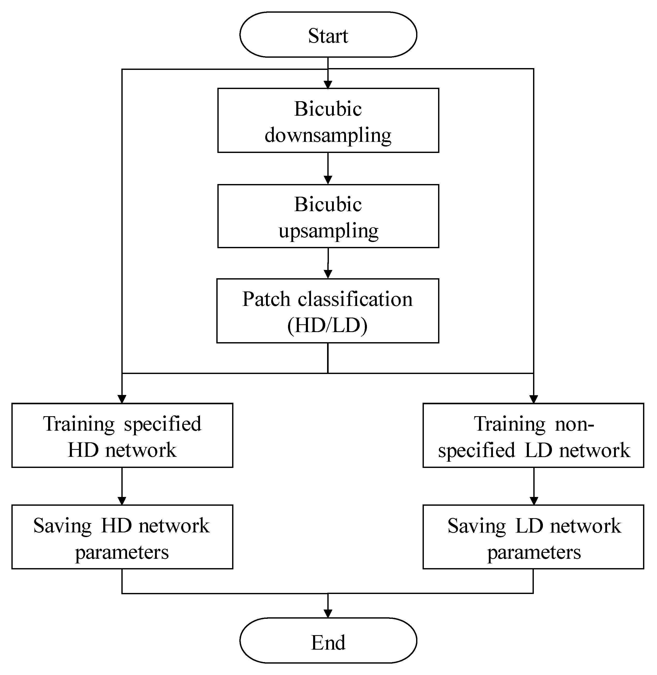
Figure 14 presents a flow chart for the simultaneous learning of the specified and non-specified neural networks. A set of training image data is prepared, and downscaling and upscaling are successively performed using bicubic interpolation. All the patches in the upscaled input image are classified as HD and LD patches. For the HD patch with a specific angle, the specified neural network parameters are trained so that the neural network output for the blurred upscaled patch is similar to the original. Similarly, for all patches classified as LD patches, the non-specified neural network parameters are trained so that the neural network output for the blurred upscaled patch is similar to the original. By simultaneously storing the specified and non-directed neural network parameters that are learned at the same time, a low-resolution image can be converted into a high-resolution one through the adaptive DNN according to the patch orientation given in the real-time online environment. According to [10], the network training for minimizing the defined loss function was performed on NVIDIA 1080 GPU, under MATLAB with the MatConvNet package for about 24 h.

3.2. State-of-the-Art Image Super-Resolution Models

In this subsection, various state-of-the-art learning-based super-resolution algorithms [32,33,34,35,36,37,38,39,40,41,42,43,44,45,46,47,48,49], which have been recently published, are briefly summarized in terms of key ideas. In [32], the enhanced deep super-resolution (EDSR) network based on optimization by removing an unnecessary batch normalization process was proposed. The iterative up- and down-sampling architecture [33] and residual-in-residual architecture [34] were also developed for improving single image super-resolution performance. Recently, a second-order attention network (SAN) [35] was proposed to exploit the feature correlation between intermediate layers, and a dual regression network (DRN) [36] based on the additional constraint in the low-resolution domain was proposed. In [37], an adaptive importance learning scheme was applied for improving the lightweight image super-resolution network. An unsupervised image translation scheme [38] and unified maximum a posteriori (MAP) framework [39] were also proposed. In [40], a three-step hierarchical CNN was proposed to learn features from different levels. With the help of an image soft-edge that is an important image feature, the soft-edge assisted network (SeaNet) was proposed [41]. The combination of the new cross-scale non-local attention prior and a recurrent neural network (RNN) [42] and unsupervised learning in the generative adversarial network (GAN) [43] were also proposed. In [44], the kernel attention module that enables the network to adjust its receptive field size was proposed for single image super-resolution. In [45], feature refinement with a high-order attention mechanism was proposed for recovering high-resolution image details. For use by autonomous underwater robots, a deep residual network-based underwater generative super-resolution model was proposed [46]. In [47], the dual-branch model was proposed to extract base features and recovered features separately. In [48], a fusion approach was proposed for hyperspectral image super-resolution by exploiting the matrix decomposition. In [49], photo up-sampling via latent space exploration (PULSE) that generates realistic high-resolution images was proposed.

4. Quantitative Performance Comparison

To evaluate the restoration performance of the trained networks, various quantitative comparisons were conducted [4,10]. Specifically, the evaluation of image denoising performance was performed in [4], and the evaluation of image super-resolution performance was performed in [10].

Table 1. Comparison of the quantitative denoising quality of eight conventional images in terms of peak signal-to-noise ratio (PSNR) (dB) and structure similarity (SSIM).

Method	Noise Level	Metric	Cameraman	Barbara	Bird	Butterfly	Hall Monitor	Lena	Mobile	Peppers
Degraded	q = 10, peak = 200	PSNR	25.85	25.13	30.86	27.90	27.91	29.89	21.85	29.39
		SSIM	0.737	0.753	0.805	0.836	0.771	0.777	0.750	0.754
	q = 20, peak = 400	PSNR	27.67	27.46	32.84	30.17	30.28	31.82	24.16	31.15
		SSIM	0.776	0.827	0.827	0.873	0.815	0.819	0.822	0.797
	q = 30, peak = 600	PSNR	28.97	29.17	34.02	31.41	31.56	32.84	25.73	32.04
		SSIM	0.814	0.864	0.850	0.888	0.839	0.841	0.859	0.819
BM3D [51]	q = 10, peak = 200	PSNR	27.22	27.18	33.13	29.97	29.89	31.29	22.83	31.53
		SSIM	0.809	0.805	0.901	0.913	0.858	0.802	0.782	0.825
	q = 20, peak = 400	PSNR	29.16	29.69	35.70	32.38	32.20	33.08	25.43	32.93
		SSIM	0.846	0.880	0.920	0.932	0.899	0.840	0.876	0.842
	q = 30, peak = 600	PSNR	30.47	31.21	37.14	33.59	33.75	34.29	26.95	33.27
		SSIM	0.871	0.902	0.921	0.931	0.902	0.858	0.897	0.844
SSRQC [52]	q = 10, peak = 200	PSNR	27.32	27.31	33.14	30.53	29.73	31.27	23.05	31.49
		SSIM	0.814	0.821	0.891	0.913	0.853	0.805	0.794	0.818
	q = 20, peak = 400	PSNR	28.97	29.32	35.28	32.65	32.20	32.94	25.29	32.91
		SSIM	0.844	0.872	0.905	0.930	0.880	0.835	0.864	0.836
	q = 30, peak = 600	PSNR	30.18	30.91	36.38	33.63	33.36	34.27	26.74	33.61
		SSIM	0.868	0.898	0.915	0.936	0.891	0.850	0.892	0.847
ARCNN [53]	q = 10, peak = 200	PSNR	27.34	26.63	33.33	31.04	30.01	31.88	23.22	31.27
		SSIM	0.819	0.811	0.901	0.918	0.880	0.847	0.807	0.827
	q = 20, peak = 400	PSNR	28.86	29.18	35.11	33.22	32.49	33.56	25.70	32.57
		SSIM	0.838	0.873	0.906	0.931	0.898	0.872	0.868	0.848
	q = 30, peak = 600	PSNR	30.15	30.85	36.26	34.37	33.76	34.43	27.22	33.38
		SSIM	0.860	0.902	0.912	0.937	0.907	0.885	0.897	0.860
DnCNN [54]	q = 10, peak = 200	PSNR	27.81	27.15	33.50	31.17	30.52	31.92	23.60	31.55
		SSIM	0.833	0.817	0.903	0.919	0.886	0.844	0.809	0.823
	q = 20, peak = 400	PSNR	29.58	29.63	35.33	33.52	32.94	33.63	26.22	32.95
		SSIM	0.852	0.873	0.909	0.934	0.901	0.867	0.875	0.839
	q = 30, peak = 600	PSNR	30.75	31.18	36.35	34.62	33.95	34.44	27.86	33.61
		SSIM	0.870	0.897	0.913	0.938	0.905	0.877	0.906	0.847
MWCNN [55]	q = 10, peak = 200	PSNR	28.09	27.71	33.23	31.10	30.62	31.91	23.69	31.53
		SSIM	0.830	0.820	0.894	0.918	0.880	0.845	0.809	0.821
	q = 20, peak = 400	PSNR	29.68	29.92	34.85	33.26	32.74	33.35	26.15	32.72
		SSIM	0.839	0.871	0.889	0.927	0.886	0.856	0.871	0.828
	q = 30, peak = 600	PSNR	30.98	31.55	36.07	34.54	34.00	34.32	27.74	33.49
		SSIM	0.864	0.898	0.900	0.931	0.897	0.870	0.900	0.841
SCENet [4]	q = 10, peak = 200	PSNR	28.24	27.67	34.08	31.72	31.13	32.37	23.90	32.12
		SSIM	0.846	0.825	0.916	0.932	0.905	0.851	0.822	0.835
	q = 20, peak = 400	PSNR	30.20	30.32	36.41	34.21	33.85	34.25	26.54	33.68
		SSIM	0.880	0.887	0.935	0.951	0.930	0.879	0.893	0.856
	q = 30, peak = 600	PSNR	31.36	31.84	37.58	35.37	35.10	35.18	28.17	34.43
		SSIM	0.894	0.910	0.939	0.955	0.936	0.891	0.920	0.866

summarizes the peak signal-to-noise ratio (PSNR) and structure similarity (SSIM) [50] values obtained from the denoising results of eight conventional test images. For this comparison, six state-of-the-art image denoising algorithms [4,51,52,53,54,55] and several different noise levels (q and peak) were utilized. The denoising method [51] utilizes collaborative filtering based on block-matching and 3D transformation (BM3D), and the image denoising framework based on a combination of structural sparse representation and quantization constraint priors was proposed [52]. The shallow neural network was also proposed for reducing compression artifacts such as blocking and ringing artifacts [53], and the single deep learning model was proposed to tackle general image restoration tasks such as compressed image deblocking and image super-resolution [54]. In addition, the multi-level wavelet CNN (MWCNN) with the modified U-Net architecture was proposed for compressed noise reduction [55]. Executable MATLAB programs and pre-trained models of the algorithms [4,51,52,53,54,55] are available in the first authors’ websites. The pre-trained models for MWCNN [55] were kindly provided by P. Liu, because it was not available via the website. Among the algorithms [4,51,52,53,54,55], some algorithms [51,52,53] run on CPU-based hardware, and the others [4,54,55] run on high-performance GPU-based hardware. The values in Table 1 indicate that the best PSNR and SSIM values are mostly provided by the SCENet by removing compressed Poisson noises successfully. Furthermore, a quantitative comparison of the LIVE1 database was conducted, as seen in

Table 2. Comparison of the quantitative denoising quality of the LIVE1 database in terms of average PSNR (dB) and SSIM.

Noise Level	Metric	Degraded	BM3D [51]	SSRQC [52]	ARCNN [53]	DnCNN [54]	MWCNN [55]	SCENet [4]
q = 10, peak = 200	PSNR	27.01	27.85	28.03	28.16	28.60	28.64	28.97
	SSIM	0.730	0.761	0.762	0.774	0.797	0.795	0.805
q = 20, peak = 400	PSNR	28.99	30.15	29.88	30.22	30.60	30.47	31.08
	SSIM	0.794	0.833	0.835	0.843	0.850	0.841	0.863
q = 30, peak = 600	PSNR	30.18	31.38	31.30	31.35	31.58	31.63	32.34
	SSIM	0.827	0.861	0.859	0.868	0.873	0.871	0.890

. The average PSNR and SSIM values were calculated from the luminance channels of the 29 images in the database. This reveals that the SCENet [4] overall outperforms the existing compressed image denoising algorithms [51,52,53,54,55] and provides significant quality improvement compared with input degraded images.

Meanwhile, to evaluate the super-resolution performance of the trained networks, five and 14 images from the Set5 and Set14 databases, respectively, were used [10]. For this evaluation, existing image super-resolution algorithms [9,10,54,56,57] were adopted, and their restoration performances were compared. The network training in [9] was performed using ILSVRC 2013 ImageNet dataset. In [10,57], the Berkeley segmentation dataset and DIV2K dataset were used for the training. In addition, the Berkeley segmentation dataset and 291 self-collected images were used for the training in [54,56], respectively.

Table 3. Comparison of the quantitative super-resolution quality of the Set5 and Set14 databases in terms of average PSNR (dB) and SSIM.

Dataset	Scale Factor	Metric	Bicubic	SRCNN [9]	VDSR [56]	DnCNN [54]	SRMD [57]	POSNet [10]
Set5 (5 images)	×2	PSNR	33.64	36.66	37.56	37.58	37.53	37.75
		SSIM	0.929	0.954	0.959	0.959	0.959	0.961
	×3	PSNR	30.39	32.75	33.67	33.75	33.86	34.24
		SSIM	0.868	0.909	0.922	0.922	0.923	0.927
	×4	PSNR	28.42	30.49	31.35	31.40	31.59	32.06
		SSIM	0.810	0.862	0.885	0.885	0.887	0.890
Set14 (14 images)	×2	PSNR	30.22	32.45	33.02	33.03	33.12	33.28
		SSIM	0.868	0.906	0.913	0.913	0.914	0.915
	×3	PSNR	27.53	29.30	29.77	29.81	29.84	30.27
		SSIM	0.774	0.821	0.832	0.832	0.833	0.841
	×4	PSNR	25.99	27.50	27.99	28.04	28.15	28.51
		SSIM	0.702	0.751	0.766	0.767	0.772	0.779

presents the average PSNR and SSIM values computed from the upscaled images of different super-resolution algorithms on the Set5 and Set14 databases. The table values indicate that POSNet [10] provides the best quantitative quality for all cases by successfully recovering GT pixel values and structures compared with the other super-resolution algorithms [9,54,56,57]. As shown in

Table 4. Comparison of the quantitative super-resolution quality of the BSDS100, Urban100, and Manga109 databases in terms of average PSNR (dB) and SSIM.

Dataset	Scale Factor	Metric	Bicubic	EDSR [32]	DBPN [33]	RCAN [34]	SAN [35]	DRN [36]
BSDS100 (100 images)	×8	PSNR	23.67	24.80	24.90	24.96	24.88	25.00
		SSIM	0.547	0.595	0.602	0.605	0.601	0.606
Urban100 (100 images)		PSNR	20.74	22.55	22.72	22.97	22.70	22.99
		SSIM	0.515	0.618	0.631	0.643	0.631	0.644
Manga109 (109 images)		PSNR	21.47	24.54	25.14	25.23	24.85	25.33
		SSIM	0.649	0.775	0.798	0.802	0.790	0.806

, the super-resolution performance for a large-scale factor of 8 was also examined using existing state-of-the-art super-resolution algorithms [32,33,34,35,36], which provide their pre-trained models for the scale factor of 8. According to [32,33,34,35,36], the pre-trained models were commonly obtained by using a DIV2K image dataset.

Table 5. Comparison of the number of learning parameters required for super-resolution algorithms.

	Scale Factor	Bicubic	EDSR [32]	DBPN [33]	RCAN [34]	SAN [35]	DRN [36]
Number of parameters (×106)	×8	-	45.5	23.2	15.7	16.0	10.0

also shows the number of learning parameters related to the computational costs of state-of-the-art algorithms. Table 4 and Table 5 show that DRN [36] achieves the best scores among the algorithms [32,33,34,35,36] with the smallest number of learning parameters on three databases: 100 images from the BSDS100, 100 images from the Urban100, and 109 images from the Manga109. Note that all the experimental results in Table 3, Table 4 and Table 5 were taken from their published papers and compared. The experimental results of the algorithm [56] in Table 3 were also taken from the existing papers [10,54,57].

5. Conclusions

The latest image denoising neural network systems introduced in this paper improve distorted inter-block correlation using the low-frequency secondary domain DNN instead of the normal pixel or transform domain. Transform coefficients generally have different quantization step sizes for each coefficient; therefore, they have different compression levels. The adaptive reconstruction for each transform coefficient is possible when a secondary image is used. Moreover, to be robust to the spatial-variant characteristics of the compressed Poisson noise, it is possible to design a neural network comprising repeated-layer architectures with a variance stabilization function. Furthermore, the latest super-resolution imaging neural network systems propose specified and non-specified neural networks using patch-orientation information and adapt them according to the input patch orientation by arranging them in parallel. Through this, it is possible to significantly improve the super-resolution performance of the HD patch while maintaining the super-resolution performance of the LD patch. Additionally, by incorporating other techniques such as outline padding in the orientation-specified neural network and angle conversion, a neural network designated in a specific orientation can be consistently applied to the HD patch capable of having multiple orientations. For a dataset available in advance, the low-quality or low-resolution images can be effectively converted into high-definition images using a neural network trained via the framework for the simultaneous learning and storing of specified and non-specified neural network parameters. Finally, the deep learning-based technologies introduced in this paper significantly improve the image quality that may have been deteriorated owing to sensor noises, compression, blurring, and downscaling caused by image acquisition and transmission and reception systems. These technologies are expected to improve the performance of various video analysis platforms. As a future work in this research field, unified neural network models for considering both compressed Poisson noise reduction and super-resolution simultaneously can be suggested and developed. In the network models, higher noise levels and scale factors may be considered. In addition, automatic estimation processes of key parameters such as noise levels and blur kernels are required in the future for achieving practical super-high-definition imaging. Further optimization techniques based on lightweight neural networks will be also proposed for real-time super-high-definition imaging.

References

- D’Haeyer, J.P. Gaussin filtering of images: A regularization approach. Signal Process. 1989, 18, 169–181. [Google Scholar] [CrossRef]
- Tomasi, C.; Manduchi, R. Bilateral filtering for gray and color images. In Proceedings of the IEEE International Conference on Computer Vision, Bombay, India, 11–18 January 1998; pp. 839–846. [Google Scholar]
- Yoo, S.B.; Han, M. DVSNet: Deep variance-stabilised network robust to spatially variant characteristics in imaging. Electron. Lett. 2019, 55, 529–531. [Google Scholar] [CrossRef]
- Yoo, S.B.; Han, M. SCENet: Secondary domain intercorrelation enhanced network for alleviating compressed Poisson noises. Sensors 2019, 19, 1939. [Google Scholar] [CrossRef] [Green Version]
- Markku, M.; Foi, A. Optimal inversion of the Anscombe transformation in low-count Poisson image denoising. IEEE Trans. Image Process. 2011, 20, 99–109. [Google Scholar]
- Freeman, W.T.; Jones, T.R.; Pasztor, E.C. Example-based super-resolution. IEEE Comput. Graph. 2002, 22, 56–65. [Google Scholar] [CrossRef] [Green Version]
- Kim, C.; Choi, K.; Ra, J.B. Example-based super-resolution via structure analysis of patches. IEEE Signal Process. Lett. 2013, 20, 407–410. [Google Scholar] [CrossRef]
- Glasner, D.; Bagon, S.; Irani, M. Super-resolution from a single image. In Proceedings of the IEEE Conference on Computer Vision and Pattern Recognition, Miami Beach, FL, USA, 20–25 June 2009; pp. 349–356. [Google Scholar]
- Dong, C.; Loy, C.C.; He, K.; Tang, X. Image super-resolution using deep convolutional networks. IEEE Trans. Pattern Anal. Mach. Intell. 2015, 38, 295–307. [Google Scholar]
- Yoo, S.B.; Han, M. Patch orientation-specified network for learning-based image super-resolution. Electron. Lett. 2019, 55, 1233–1235. [Google Scholar] [CrossRef]
- Yang, W.; Zhang, X.; Tian, Y.; Wang, W.; Xue, J.H.; Liao, Q. Deep learning for single image super-resolution: A brief review. IEEE Trans. Multimed. 2019, 21, 3106–3121. [Google Scholar] [CrossRef] [Green Version]
- Zhao, S.; Shmaliy, Y.S.; Liu, F. Fast computation of discrete optimal FIR estimates in white Gaussian noise. IEEE Signal Process. Lett. 2014, 22, 718–722. [Google Scholar] [CrossRef]
- Shabalin, A.A.; Nobel, A.B. Reconstruction of a low-rank matrix in the presence of Gaussian noise. J. Multivar. Anal. 2013, 118, 67–76. [Google Scholar] [CrossRef] [Green Version]
- Deledalle, C.A.; Denis, L.; Tupin, F. How to compare noisy patches? Patch similarity beyond Gaussian noise. Int. J. Comput. Vis. 2012, 99, 86–102. [Google Scholar] [CrossRef] [Green Version]
- Wang, Y.Q.; Morel, J.M. Can a single image denoising neural network handle all levels of Gaussian noise? IEEE Signal Process. Lett. 2014, 21, 1150–1153. [Google Scholar] [CrossRef]
- Salmon, J.; Harmany, Z.; Deledalle, C.A.; Willett, R. Poisson noise reduction with non-local PCA. J. Math. Imaging Vis. 2014, 48, 279–294. [Google Scholar] [CrossRef] [Green Version]
- Giryes, R.; Elad, M. Sparsity-based Poisson denoising with dictionary learning. IEEE Trans. Image Process. 2014, 23, 5057–5069. [Google Scholar] [CrossRef] [Green Version]
- Luisier, F.; Blu, T.; Unser, M. Image denoising in mixed Poisson–Gaussian noise. IEEE Trans. Image Process. 2010, 20, 696–708. [Google Scholar] [CrossRef] [Green Version]
- Makitalo, M.; Foi, A. Optimal inversion of the generalized Anscombe transformation for Poisson-Gaussian noise. IEEE Trans. Image Process. 2012, 22, 91–103. [Google Scholar] [CrossRef]
- Le, Y.; Angelini, E.D.; Olivo-Marin, J.C. An unbiased risk estimator for image denoising in the presence of mixed Poisson–Gaussian noise. IEEE Trans. Image Process. 2014, 23, 1255–1268. [Google Scholar]
- Zhang, Y.; Zhu, Y.; Nichols, E.; Wang, Q.; Zhang, S.; Smith, C.; Howard, S. A Poisson-Gaussian denoising dataset with real fluorescence microscopy images. In Proceedings of the IEEE Conference on Computer Vision and Pattern Recognition, Long Beach, CA, USA, 16–20 June 2019; pp. 11710–11718. [Google Scholar]
- Zhou, Z. Cognition and removal of impulse noise with uncertainty. IEEE Trans. Image Process. 2012, 21, 3157–3167. [Google Scholar] [CrossRef]
- Lien, C.Y.; Huang, C.C.; Chen, P.Y.; Lin, Y.F. An efficient denoising architecture for removal of impulse noise in images. IEEE Trans. Comput. 2012, 62, 631–643. [Google Scholar] [CrossRef]
- Chen, Y.; Zhang, Y.; Shu, H.; Yang, J.; Luo, L.; Coatrieux, J.L.; Feng, Q. Structure-adaptive fuzzy estimation for random-valued impulse noise suppression. IEEE Trans. Circuits Sys. Video Technol. 2016, 28, 414–427. [Google Scholar] [CrossRef]
- Chen, C.L.P.; Liu, L.; Chen, L.; Tang, Y.Y.; Zhou, Y. Weighted couple sparse representation with classified regularization for impulse noise removal. IEEE Trans. Image Process. 2015, 24, 4014–4026. [Google Scholar] [CrossRef] [PubMed]
- Yoo, S.B.; Choi, K.; Ra, J.B. Post-processing for blocking artifact reduction based on inter-block correlation. IEEE Trans. Multimed. 2014, 16, 1536–1548. [Google Scholar] [CrossRef]
- Yoo, S.B.; Choi, K.; Ra, J.B. Blind post-processing for ringing and mosquito artifact reduction in coded videos. IEEE Trans. Circuits Syst. Video Technol. 2014, 24, 721–732. [Google Scholar]
- Yoo, S.B.; Choi, K.; Ra, J.B. Post processing for blocking artifact reduction. In Proceedings of the IEEE International Conference on Image Processing, Brussels, Belgium, 11–14 September 2011; pp. 1509–1512. [Google Scholar]
- Zhang, J.; Xiong, R.; Zhao, C.; Zhang, Y.; Ma, S.; Gao, W. CONCOLOR: Constrained non-convex low-rank model for image deblocking. IEEE Trans. Image Process. 2016, 25, 1246–1259. [Google Scholar] [CrossRef]
- Norkin, A.; Bjontegaard, G.; Fuldseth, A.; Narroschke, M.; Ikeda, M.; Andersson, K.; Van, G. HEVC deblocking filter. IEEE Trans. Circuits Syst. Video Technol. 2012, 22, 1746–1754. [Google Scholar] [CrossRef]
- Zhao, Z.; Sun, Q.; Yang, H.; Qiao, H.; Wang, Z.; Wu, D.O. Compression artifacts reduction by improved generative adversarial networks. Eurasip J. Image Video 2019, 1, 1–7. [Google Scholar] [CrossRef]
- Lim, B.; Son, S.; Kim, H.; Nah, S.; Lee, K.M. Enhanced deep residual networks for single image super-resolution. In Proceedings of the IEEE Conference on Computer Vision and Pattern Recognition Workshops, Honolulu, GA, USA, 21–26 July 2017; pp. 136–144. [Google Scholar]
- Haris, M.; Shakhnarovich, G.; Ukita, N. Deep back-projection networks for super-resolution. In Proceedings of the IEEE Conference on Computer Vision and Pattern Recognition, Salt Lake City, UT, USA, 18–22 June 2018; pp. 1664–1673. [Google Scholar]
- Zhang, Y.; Li, K.; Li, K.; Wang, L.; Zhong, B.; Fu, Y. Image super-resolution using very deep residual channel attention networks. In Proceedings of the IEEE European Conference on Computer Vision, Munich, Germany, 8–14 September 2018; pp. 286–301. [Google Scholar]
- Dai, T.; Cai, J.; Zhang, Y.; Xia, S.T.; Zhang, L. Second-order attention network for single image super-resolution. In Proceedings of the IEEE Conference on Computer Vision and Pattern Recognition, Long Beach, CA, USA, 16–20 June 2019; pp. 11065–11074. [Google Scholar]
- Guo, Y.; Chen, J.; Wang, J.; Chen, Q.; Cao, J.; Deng, Z.; Xu, Y.; Tan, M. Closed-loop matters: Dual regression networks for single image super-resolution. In Proceedings of the IEEE/CVF Conference on Computer Vision and Pattern Recognition, Virtual, Seattle, WA, USA, 14–19 June 2020; pp. 5407–5416. [Google Scholar]
- Zhang, L.; Wang, P.; Shen, C.; Liu, L.; Wei, W.; Zhang, Y.; Van, A. Adaptive importance learning for improving lightweight image super-resolution network. Int. J. Comput. Vis. 2020, 128, 479–499. [Google Scholar] [CrossRef] [Green Version]
- Chen, S.; Han, Z.; Dai, E.; Jia, X.; Liu, Z.; Xing, L.; Tian, Q. Unsupervised image super-resolution with an indirect supervised path. In Proceedings of the IEEE/CVF Conference on Computer Vision and Pattern Recognition Workshops, Seattle, WA, USA, 14–19 June 2020; pp. 468–469. [Google Scholar]
- Zhang, K.; Gool, L.V.; Timofte, R. Deep unfolding network for image super-resolution. In Proceedings of the IEEE/CVF Conference on Computer Vision and Pattern Recognition Workshops, Seattle, WA, USA, 14–19 June 2020; pp. 3217–3226. [Google Scholar]
- Liu, B.; Ait-Boudaoud, D. Effective image super resolution via hierarchical convolutional neural network. Neurocomputing 2020, 374, 109–116. [Google Scholar] [CrossRef]
- Fang, F.; Li, J.; Zeng, T. Soft-edge assisted network for single image super-resolution. IEEE Trans. Image Process. 2020, 29, 4656–4668. [Google Scholar] [CrossRef]
- Mei, Y.; Fan, Y.; Zhou, Y.; Huang, L.; Huang, T.S.; Shi, H. Image super-resolution with cross-scale non-local attention and exhaustive self-exemplars mining. In Proceedings of the IEEE/CVF Conference on Computer Vision and Pattern Recognition, Seattle, WA, USA, 14–19 June 2020; pp. 5690–5699. [Google Scholar]
- Prajapati, K.; Chudasama, V.; Patel, H.; Upla, K.; Ramachandra, R.; Raja, K.; Busch, C. Unsupervised single image super-resolution network (USISRESNET) for real-world data using generative adversarial network. In Proceedings of the IEEE/CVF Conference on Computer Vision and Pattern Recognition Workshops, Seattle, WA, USA, 14–19 June 2020; pp. 464–465. [Google Scholar]
- Zhang, D.; Shao, J.; Shen, H.T. Kernel attention network for single image super-resolution. ACM Trans. Multim. Comput. 2020, 16, 1–15. [Google Scholar]
- Zhang, D.; Shao, J.; Li, X.; Shen, H.T. Remote sensing image super-resolution via mixed high-order attention network. IEEE Trans. Geosci. Remote Sens. 2020, 1–14. [Google Scholar] [CrossRef]
- Islam, M.J.; Enan, S.S.; Luo, P.; Sattar, J. Underwater image super-resolution using deep residual multipliers. In Proceedings of the IEEE International Conference on Robotics and Automation, Xi’an, China, 31 May 2020; pp. 900–906. [Google Scholar]
- Zhang, X.; Dong, H.; Hu, Z.; Lai, W.S.; Wang, F.; Yang, M.H. Gated fusion network for degraded image super resolution. Int. J. Comput. Vis. 2020, 128, 1–23. [Google Scholar] [CrossRef] [Green Version]
- Liu, J.; Wu, Z.; Xiao, L.; Sun, J.; Yan, H. A truncated matrix decomposition for hyperspectral image super-resolution. IEEE Trans. Image Process. 2020, 29, 8028–8042. [Google Scholar] [CrossRef]
- Menon, S.; Damian, A.; Hu, S.; Ravi, N.; Rudin, C. PULSE: Self-supervised photo upsampling via latent space exploration of generative models. In Proceedings of the IEEE/CVF Conference on Computer Vision and Pattern Recognition Workshops, Seattle, WA, USA, 14–19 June 2020; pp. 2437–2445. [Google Scholar]
- Wang, Z.; Bovik, A.C.; Sheikh, H.R.; Simoncelli, E.P. Image quality assessment: From error visibility to structural similarity. IEEE Trans. Image Process. 2004, 13, 600–612. [Google Scholar] [CrossRef] [Green Version]
- Dabov, K.; Foi, A.; Katkovnik, V.; Egiazarian, K. Image denoising by sparse 3-D transform-domain collaborative filtering. IEEE Trans. Image Process. 2007, 16, 2080–2095. [Google Scholar] [CrossRef]
- Zhao, C.; Zhang, J.; Ma, S.; Fan, X.; Zhang, Y.; Gao, W. Reducing image compression artifacts by structural sparse representation and quantization constraint prior. IEEE Trans. Circuits Syst. Video Technol. 2017, 27, 2057–2071. [Google Scholar] [CrossRef]
- Dong, C.; Deng, Y.; Change, L.C.; Tang, X. Compression artifacts reduction by a deep convolutional network. In Proceedings of the IEEE International Conference on Computer Vision, Santiago, Chile, 11–18 December 2015; pp. 576–584. [Google Scholar]
- Zhang, K.; Zuo, W.; Chen, Y.; Meng, D.; Zhang, L. Beyond a Gaussian denoiser: Residual learning of deep CNN for image denoising. IEEE Trans. Image Process. 2017, 26, 3142–3155. [Google Scholar] [CrossRef] [Green Version]
- Liu, P.; Zhang, H.; Zhang, K.; Lin, L.; Zuo, W. Multi-level wavelet-CNN for image restoration. In Proceedings of the IEEE Conference on Computer Vision and Pattern Recognition Workshops, Salt Lake City, UT, USA, 18–22 June 2018; pp. 773–782. [Google Scholar]
- Kim, J.; Lee, J.K.; Lee, K.M. Accurate image super-resolution using very deep convolutional networks. In Proceedings of the IEEE Conference on Computer Vision and Pattern Recognition, Las Vegas, NV, USA, 26–30 June 2016; pp. 1646–1654. [Google Scholar]
- Zhang, K.; Zuo, W.; Zhang, L. Learning a single convolutional super-resolution network for multiple degradations. In Proceedings of the IEEE Conference on Computer Vision and Pattern Recognition, Salt Lake City, UT, USA, 18–22 June 2018; pp. 3262–3271. [Google Scholar]
Figure 1.
The numbers of publications on image super-resolution, image denoising, and ultra-high-definition.
Figure 2.
Image degradation model owing to the coding of Poisson noisy images.
Figure 3.
Example of noise estimation using sample mean.
Figure 4.
Spatial variation of local standard deviation (STD) of the estimated noise.
Figure 5.
Intercorrelation distribution according to compression level.
Figure 6.
Architecture of the secondary domain intercorrelation enhanced network [4].
Figure 7.
Applications of the image super-resolution technique.
Figure 8.
Classification of the approach to image super-resolution.
Figure 9.
Example-based super-resolution using external learning [6].
Figure 10.
Example-based super-resolution using structure analysis of patches [7].
Figure 11.
Example-based super-resolution using internal learning [8].
Figure 12.
Deep learning-based super-resolution [9].
Figure 13.
Architecture of the patch orientation-specified network [10].
Figure 14.
Architecture for simultaneous learning of patch orientation-specified and non-specified neural networks [10].