Efficient Computation of the Nonlinear Schrödinger Equation with Time-Dependent Coefficients

Abstract

Motivated by the limited work performed on the development of computational techniques for solving the nonlinear Schrödinger equation with time-dependent coefficients, we develop a modified Runge–Kutta pair with improved periodicity and stability characteristics. Additionally, we develop a modified step size control algorithm, which increases the efficiency of our pair and all other pairs included in the numerical experiments. The numerical results on the nonlinear Schrödinger equation with a periodic solution verified the superiority of the new algorithm in terms of efficiency. The new method also presents a good behaviour of the maximum absolute error and the global norm in time, even after a high number of oscillations.

1. Introduction

We consider the following dimensionless form of the nonlinear Schrödinger (NLS) equation:

$$i\frac{\partial \psi }{\partial t}+a\left(t\right)\frac{{\partial }^2\psi }{\partial x^2}+b\left(t\right){\left|\psi \right|}^2\psi =0.$$

(1)

Equation (1) represents atomic Bose–Einstein condensates (BECs), where $\psi$ represents the mean-field function of the matter-wave, t is the time and x the longitudinal coordinate. Furthermore, Equation (1) can also be applied in the context of nonlinear optics [1], for the study of optical beams, in which case, $\psi$ represents the complex electric field envelope, t is the propagation distance and x is the transverse coordinate [2,3]. The varying coefficients $a\left(t\right)$ and $b\left(t\right)$ denote the dispersion and nonlinearity, respectively.

The solution $\psi (x,t)$ of Equation (1) satisfies the global norm conservation law [4]:

$$E\left(\psi \right)=\underset{\mathbb{R}}{\int }{\left|\psi (x,t)\right|}^{2}dx=\mathrm{constant}.$$

(2)

The analytical solution of the NLS with varying coefficients has attracted great interest in the recent past (e.g., see [5,6,7] or more recent works in [8,9,10,11] and references therein). Additionally, the computation of the NLS is a critical part of the verification process of the analytical theories. This has been achieved in the case of non-varying coefficients, with success for a large number of comparative numerical algorithms [12,13,14,15,16].

Other work performed on the computation of NLS with varying coefficients is limited, especially when they have a periodic/oscillatory behaviour in time. In the work of Serkin and Hasegawa in [17], a set of new soliton solutions of the NLS are found, which allow the investigation of special cases. Some of these introduce solitary solutions with periodic-oscillatory nature and are investigated by Hong and Liu in [4], along with a conservation law for a varying-coefficient NLS. On the other hand, Tang et al. create a predictor-corrector method for the NLS with varying coefficients in [18].

In general, for initial/boundary problems that present a periodic/oscillatory behaviour, a very popular and efficient computational approach is using the method of lines, where the numerical algorithm used for the time integration is specifically designed for this behaviour. Among these time steppers, very wide-spread are the ones with variable coefficients, such as phase-fitted and/or amplification-fitted, trigonometrically-fitted etc. (e.g., [19,20,21,22,23,24,25]). This approach requires a well-defined dominant frequency of the oscillations along the propagation coordinate and, when this is not the case, they under-perform. A different approach is to construct optimised numerical methods that have constant coefficients, which do not rely on the knowledge of the frequencies of the problem (e.g., [26,27,28,29,30,31]). Following these techniques, no fitting is performed. Instead, properties such as the phase-lag, commonly also referred to as dispersion error, and the amplification-error, commonly also referred to as dissipation error, are optimised.

Another methodology that is used along with single-step methods is the step size control, which allows the method to automatically adjust the step size and thus reduce the computation effort [19,20,21,22,23,26,29,31,32,33,34,35,36]. For some types of methods, the local error estimation can be performed using an embedded estimator, which has many advantages over other techniques, such as extrapolation [32]. For Runge–Kutta (RK) methods, this estimation can be very cheap computationally, since a second approximation is performed using the same internal stages of the method, with negligible additional cost.

In this article, we construct an explicit 6(4)-order, eight-stage Runge–Kutta pair with constant coefficients that has increased phase-lag and amplification-error orders and stability intervals. The values of the coefficients have deliberately chosen to have similar orders of magnitude, to minimise the round-off error. Additionally, the low-order method is developed with similar stability characteristics to the high-order one, to improve the local error estimation for extreme step sizes. For a complete list of the criteria satisfied, see Section 3.

Additionally, we develop a modified step size control algorithm, specifically designed for the NLS equation, which increases the efficiency of our pair and all other pairs included in the numerical experiments. For its development, see Section 4.

The structure of this paper is as follows:

• in Section 2 required basic theory concepts are reported;
• Section 3 shows the construction and the analysis of the new RK pair;
• in Section 4 we present the new modified step size control algorithm;
• in Section 5 we present the numerical experiments on the NLS;
• in Section 6 we discuss conclusions.

2. Theory

2.1. Explicit Runge–Kutta Pairs

A Runge–Kutta method is considered an extension of the Euler method that provides a more accurate approximation by the use of additional derivative evaluations. To achieve a certain algebraic order p, then the following set of equations must hold $y^{\left(n\right)}\left(x\right)=y_n^{\left(n\right)}\left(x\right),n=1,2,\cdots ,p$, where y and $y_n$ are the theoretical and numerical solutions, respectively.

For the numerical solution of Equation (1), let $(x,t)\in [x_L,x_R]\times [0,T]$. If $y_m^{n+1}$ and ${\widehat{y}}_m^{n+1}$ denote approximations of $\psi (x_m,t_{n+1})$, where $x_m=x_L+m\mathrm{\Delta }x$, $m=0,1,\dots ,M-1$, $t_{n+1}=t_n+h,n=0,1,\dots ,N-1$, then an $s-$stage embedded $q\left(p\right)s$ Runge–Kutta pair is presented in Equation (3) and consists of two methods of different orders: the high-order $(\mathbf{c},\mathbf{A},\mathbf{b})$ and the low-order $(\mathbf{c},\mathbf{A},\widehat{\mathbf{b}})$ of orders q and p, respectively, with $p<q$:

$$\left\{\begin{array}{c}{y}_m^{n+1}=y_m^n+h{\displaystyle \sum _{i=1}^s}{b}_i{k}_i\hfill \\ {\widehat{y}}_m^{n+1}=y_m^n+h{\displaystyle \sum _{i=1}^s}{\widehat{b}}_i{k}_i\hfill \\ k_i=f(t_n+c_{i}h,y_m^n+h{\displaystyle \sum _{j=1}^{i-1}}{a}_{ij}{k}_j),i=1,\dots ,s\hfill \end{array}\right.or\begin{array}{cc}\mathbf{c}& \mathbf{A}\\ & \mathbf{b}\\ & \widehat{\mathbf{b}},\end{array}$$

(3)

where $\mathbf{A}=\left[a_{ij}\right]$, $\mathbf{b}=\left[b_i\right]$, $\widehat{\mathbf{b}}=\left[{\widehat{b}}_i\right]$, $\mathbf{c}=\left[c_i\right]$, $i=1,2,\dots ,s$ and $j=1,2,\dots ,i-1$ are the coefficient matrices, h is the step size and f is defined in $y^{\prime }=f(x,y)$.

The values of y and $\widehat{y}$ are yielded by the high- and low-order methods respectively. $\widehat{y}$ only contributes to the local truncation error estimation (the step size control is discussed in Section 4).

According to rooted tree analysis [37], there are 37 equations that must be satisfied to obtain a Runge–Kutta method of sixth algebraic order:

$$\begin{array}{c}{\displaystyle \sum _{i=1}^s}{b}_i=1,{\displaystyle \sum _{i=1}^s}{b}_i{c}_i=\frac{1}{2},{\displaystyle \sum _{i=1}^s}{b}_i{c}_i^2=\frac{1}{3},{\displaystyle \sum _{i,j=1}^s}{b}_i{a}_{ij}{c}_j=\frac{1}{6},{\displaystyle \sum _{i=1}^s}{b}_i{c}_i^3=\frac{1}{4},{\displaystyle \sum _{i,j=1}^s}{b}_i{c}_i{a}_{ij}{c}_j=\frac{1}{8},{\displaystyle \sum _{i,j=1}^s}{b}_i{a}_{ij}{c}_j^2=\frac{1}{12},\hfill \\ {\displaystyle \sum _{i,j,k=1}^s}{b}_i{a}_{ij}{a}_{jk}{c}_k=\frac{1}{24},{\displaystyle \sum _{i=1}^s}{b}_i{c}_i^4=\frac{1}{5},{\displaystyle \sum _{i,j=1}^s}{b}_i{c}_i^2{a}_{ij}{c}_j=\frac{1}{10},{\displaystyle \sum _{i,j=1}^s}{b}_i{c}_i{a}_{ij}{c}_j^2=\frac{1}{15},{\displaystyle \sum _{i,j,k=1}^s}{b}_i{c}_i{a}_{ij}{a}_{jk}{c}_k=\frac{1}{30},\hfill \\ {\displaystyle \sum _{i,j=1}^s}{b}_i{a}_{ij}{c}_j^3=\frac{1}{20},{\displaystyle \sum _{i,j,k=1}^s}{b}_i{a}_{ij}{c}_j{a}_{jk}{c}_k=\frac{1}{40},{\displaystyle \sum _{i,j,k=1}^s}{b}_i{a}_{ij}{a}_{jk}{c}_k^2=\frac{1}{60},{\displaystyle \sum _{i,j,k,l=1}^s}{b}_i{a}_{ij}{a}_{jk}{a}_{kl}{c}_l=\frac{1}{120},\hfill \\ {\displaystyle \sum _{i,j,k=1}^s}{b}_i{a}_{ij}{c}_j{a}_{ik}{c}_k=\frac{1}{20},{\displaystyle \sum _{i=1}^s}{b}_i{c}_i^5=\frac{1}{6},{\displaystyle \sum _{i,j=1}^s}{b}_i{c}_i^3{a}_{ij}{c}_j=\frac{1}{12},{\displaystyle \sum _{i,j=1}^s}{b}_i{c}_i^2{a}_{ij}{c}_j^2=\frac{1}{18},{\displaystyle \sum _{i,j,k=1}^s}{b}_i{c}_i{a}_{ij}{c}_j{a}_{ik}{c}_k=\frac{1}{24},\hfill \\ {\displaystyle \sum _{i,j,k=1}^s}{b}_i{c}_i^2{a}_{ij}{a}_{jk}{c}_k=\frac{1}{36},{\displaystyle \sum _{i,j=1}^s}{b}_i{c}_i{a}_{ij}{c}_j^3=\frac{1}{24},{\displaystyle \sum _{i,j,k=1}^s}{b}_i{c}_i{a}_{ij}{c}_j{a}_{jk}{c}_k=\frac{1}{48},{\displaystyle \sum _{i,j,k=1}^s}{b}_i{a}_{ij}{c}_j{a}_{ik}{c}_k^2=\frac{1}{36},\hfill \\ {\displaystyle \sum _{i,j,k,l=1}^s}{b}_i{c}_i{a}_{ij}{a}_{jk}{a}_{kl}{c}_l=\frac{1}{144},{\displaystyle \sum _{i,j,k,l=1}^s}{b}_i{a}_{ij}{c}_j{a}_{ik}{a}_{kl}{c}_l=\frac{1}{72},{\displaystyle \sum _{i,j,k=1}^s}{b}_i{c}_i{a}_{ij}{a}_{jk}{c}_k^2=\frac{1}{72},{\displaystyle \sum _{i,j=1}^s}{b}_i{a}_{ij}{c}_j^4=\frac{1}{30},\hfill \\ {\displaystyle \sum _{i,j,k=1}^s}{b}_i{a}_{ij}{c}_j^2{a}_{jk}{c}_k=\frac{1}{60},{\displaystyle \sum _{i,j,k=1}^s}{b}_i{a}_{ij}{c}_j{a}_{jk}{c}_k^2=\frac{1}{90},{\displaystyle \sum _{i,j,k,l=1}^s}{b}_i{a}_{ij}{c}_j{a}_{jk}{a}_{kl}{c}_l=\frac{1}{180},{\displaystyle \sum _{i,j,k,l=1}^s}{b}_i{a}_{ij}{a}_{jk}{c}_k{a}_{jl}{c}_l=\frac{1}{120},\hfill \\ {\displaystyle \sum _{i,j,k=1}^s}{b}_i{a}_{ij}{a}_{jk}{c}_k^3=\frac{1}{120},{\displaystyle \sum _{i,j,k,l=1}^s}{b}_i{a}_{ij}{a}_{jk}{c}_k{a}_{kl}{c}_l=\frac{1}{240},{\displaystyle \sum _{i,j,k,l=1}^s}{b}_i{a}_{ij}{a}_{jk}{a}_{kl}{c}_l^2=\frac{1}{360},\hfill \\ {\displaystyle \sum _{i,j,k,l,m=1}^s}{b}_i{a}_{ij}{a}_{jk}{a}_{kl}{a}_{lm}{c}_m=\frac{1}{720}.\hfill \end{array}$$

(4)

Additionally, equations $c_i={\displaystyle \sum _{j=1}^s}{a}_{ij},i=1,\dots ,s$ should hold.

2.2. Phase-Lag and Stability

When dealing with initial value problems of oscillatory/periodic nature, it is critical to optimise the numerical method for solving these exact problems. This, however, is often very complicated or even impossible, due to the complexity of the problem, in addition to having developed a very problem-specific algorithm with limited applications. An efficient way to produce methods that are optimised for periodic problems is to deal with a test problem that has similar behaviour but at the same time is simple enough to produce useful results. One test problem that possesses such properties is

$$y^{\prime }=i\omega y,y\left(0\right)=y_0\omega ,y_0\in \mathbb{R},$$

(5)

with exact solution $y\left(t\right)=y_0{e}^{i\omega t}$, which represents the circular orbit on the complex plane and $\omega$ its frequency.

Equation (5) solved numerically by the RK high-order method of Equation (3) yields the solution $y_m^{n+1}=R^n{y}_m^n$, where $R\left(v\right)=A_s\left(v^2\right)+iv{B}_s\left(v^2\right)$ is called the stability polynomial, $v=\omega h$ and $A_s,B_s$ are polynomials in $v^2$. The exact solution of Equation (5) satisfies the relation $\tilde{y}\left(t_{n+1}\right)=\tilde{y}\left(t_n\right)e^{i{v}_n}$. For a generic $v=v_n$, since $|e^{iv}|=1$ and $arg\left(e^{iv}\right)=v$ we have:

Definition 1.

[38] For the s-stage Runge–Kutta method of Equation (3), $\varphi \left(v\right)=v-arg\left[R\right(v\left)\right]$ and $a\left(v\right)=1-\left|R\right(v\left)\right|$ are called the phase-lag or dispersion error and the amplification error or dissipative error, respectively. A method has dispersive order m and dissipative order r if $\varphi \left(v\right)=O\left(v^{m+1}\right)$ and $a\left(v\right)=O\left(v^{r+1}\right)$.

The phase-lag measures the error of the angle and the amplification error measures the error of the radius, as the numerical method approximates the circular orbit of Equation (5).

Definition 2.

[26] For the Runge–Kutta method of Equation (3), if $\left|R\right(i{v}_I\left)\right|<1$ and $\left|R\right(v_I+ϵ\left)\right|>1$, for every $v\in I_I$ and every suitably small positive ϵ, then the imaginary stability interval is $I_I=(0,v_I)$.

Definition 3.

For the method of Equation (3), if $\left|R\right(v_R\left)\right|<1$ and $\left|R\right(v_R-ϵ\left)\right|>1$, for every $v\in I_R$ and every suitably small positive ϵ, then the real stability interval is $I_R=(v_R,0)$.

Definition 4.

The stability region is defined as the set $S=\left\{z\in \mathbb{C}:\left|R\right(z\left)\right|<1\right\}$.

3. Construction and Analysis

For the construction of the new pair, we satisfy the following criteria:

• Sixth algebraic order, which implies the 37 equations of Equation (4) for the algebraic conditions and 7 additional equations for the eight internal stages [37].
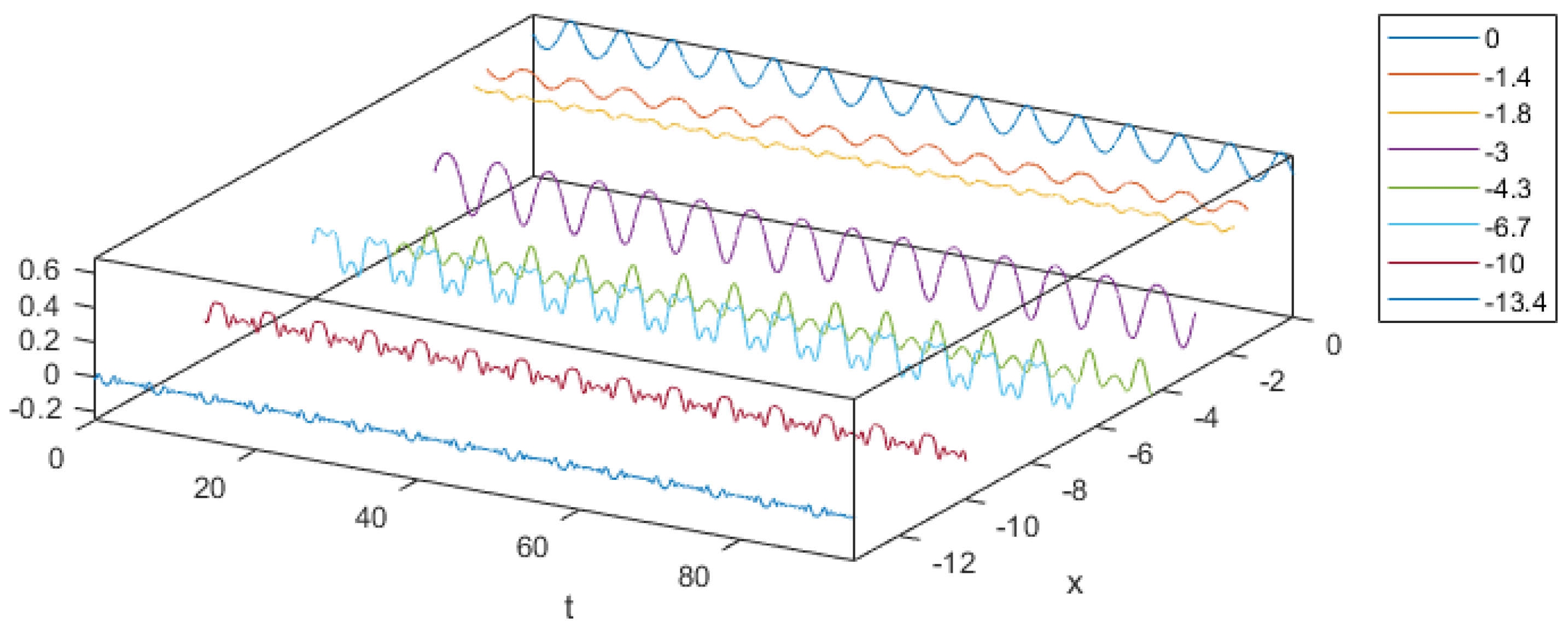
• Constant coefficients, since no dominant frequency exists for different values of x, as observed in Figure 1.
• Maximised phase-lag and amplification-error orders m and r of Definition 1, for improved behaviour when solving Equation (1) with periodic/oscillatory solutions.
• Maximised real stability interval, based on Definition 4.
• Coefficients with similar orders of magnitude, to minimise the round-off error.
• Low-order method with similar stability characteristics to the high-order one, to improve the local error estimation for extreme step sizes.

From a number of solutions that satisfy the restrictions of criteria (1) and (2), we select the one that maximises the order of phase-lag and amplification-error, i.e., criterion (3), maximises the real stability interval, i.e., criterion (4) and finally selects the values of coefficients to have similar orders of magnitude, i.e., criterion (5), in this order. Additionally, we chose the coefficients $\widehat{b}$ of the low-order method, as presented in the last row of

Table 1. The Butcher tableau of the new 6(4)8 Runge–Kutta pair.

0
$\frac{1}{15}$	$\frac{1}{15}$
$\frac{1}{5}$	$-\frac{1}{10}$	$\frac{3}{10}$
$\frac{1}{3}$	$\frac{62-5\sqrt{65}}{126}$	$\frac{-55+5\sqrt{65}}{84}$	$\frac{125-5\sqrt{65}}{252}$
$\frac{2}{5}$	$\frac{249-15\sqrt{65}}{350}$	$\frac{-141+9\sqrt{65}}{140}$	$\frac{89-3\sqrt{65}}{140}$	$\frac{3}{50}$
$\frac{3}{5}$	$\frac{192-7\sqrt{65}}{350}$	$\frac{-687+9\sqrt{65}}{700}$	$\frac{1019+37\sqrt{65}}{700}$	$-\frac{324+18\sqrt{65}}{175}$	$\frac{50+2\sqrt{65}}{35}$
$\frac{4}{5}$	$\frac{-2047+90\sqrt{65}}{1750}$	$\frac{591-27\sqrt{65}}{350}$	$\frac{285+18\sqrt{65}}{700}$	$-\frac{1071}{1000}$	$\frac{21}{50}$	$\frac{21}{40}$
1	$\frac{396-15\sqrt{65}}{119}$	$\frac{-1020+45\sqrt{65}}{238}$	$\frac{225-30\sqrt{65}}{476}$	$-\frac{3261}{952}$	$\frac{225}{34}$	$-\frac{375}{136}$	$\frac{125}{119}$
b	$\frac{5}{96}$	0	$\frac{125}{288}$	$-\frac{81}{112}$	$\frac{125}{144}$	0	$\frac{625}{2016}$	$\frac{17}{288}$
$\widehat{b}$	$\frac{5}{96}$	0	$\frac{383}{960}$	$-\frac{333}{640}$	$\frac{947}{1440}$	$\frac{101}{1920}$	$\frac{3}{10}$	$\frac{17}{288}$

, to satisfy criterion (6).

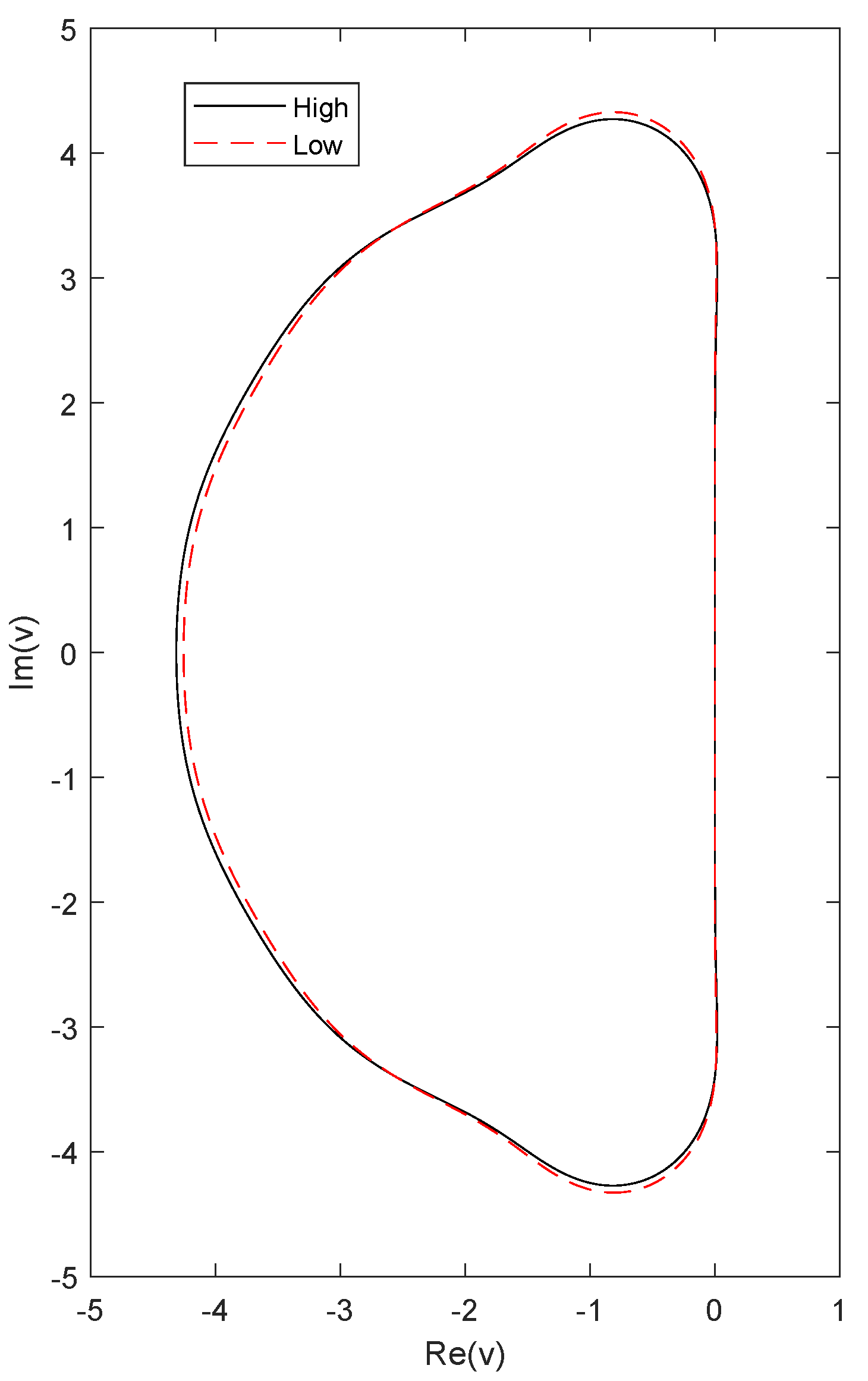
The stability regions of both high-order and low-order methods of the new pair, based on Definition 4, are presented in Figure 2. The real stability intervals of the high-order and low-order methods are ($-4.31,0$) and ($-4.25,0$) respectively. This satisfies criterion (6). The phase-lag orders of the new pair, based on Definition 1, are 8(4), while the amplification-error orders are 9(5). The coefficients of the new RK pair are presented in Table 1.

4. A Modified Step Size Control Algorithm

There are various algorithms regarding the selection of the step size, when a local error estimation is known (see e.g., [32] and references therein). The most well-known is the following:

Provided a step size $h_n$, each subsequent step size $h_{n+1}$ of the pair in Equation (3) is determined by

$${\displaystyle h_{n+1}=min\left(max\left(h_{opt},\frac{h_n}{r_{max}}\right),h_n{r}_{max}\right),where{h}_{opt}=0.9h_n{\left(\frac{TOL}{EST{h}^g}\right)}^{\frac{1}{p+1}}and}$$

(6)

$$EST=\underset{m}{max}\left(|{\widehat{y}}_m^n-y_m^n|\right),m=0,1,\dots M-1,g=0,and{r}_{max}=2.$$

(7)

$TOL$ represents the tolerance or maximum allowed local error. If $EST<TOL$, then the step is accepted and the solution advances, otherwise the step is rejected and then repeated with a new step size given by Equation (6).

Here, we introduce a modification of the above algorithm, to include the difference of the squares as the local error estimation. For the pair of Equation (3), since $q⩾p+1$, we have:

$${\widehat{y}}_m^n=\psi (x_m,t_n)+C{h}^{p+1}+O\left(h^{p+2}\right)$$

(8)

and

$$y_m^n=\psi (x_m,t_n)+D{h}^{p+2}+O\left(h^{p+3}\right)$$

(9)

The nature of NLS suggests the use of

$$\begin{array}{cc}{\left({\widehat{y}}_m^n\right)}^2-{\left(y_m^n\right)}^2\hfill & \simeq {\left(\psi (x_m,t_n)+C{h}^{p+1}\right)}^2-{\left(\psi (x_m,t_n)+D{h}^{p+2}\right)}^2\hfill \\ & ={\psi }^2(x_m,t_n)+2\psi (x_m,t_n)C{h}^{p+1}+C^2{h}^{2p+2}-{\psi }^2(x_m,t_n)-2\psi (x_m,t_n)D{h}^{p+2}-D{h}^{2p+4}\hfill \\ & =2\psi (x_m,t_n)C{h}^{p+1}+O\left(h^{p+2}\right)\simeq 2\psi (x_m,t_n)C{h}^{p+1}.\hfill \end{array}$$

This means that ${\displaystyle C{h}^{p+1}\simeq \frac{{\left({\widehat{y}}_m^n\right)}^2-{\left(y_m^n\right)}^2}{2\psi (x_m,t_n)}\simeq \frac{{\left({\widehat{y}}_m^n\right)}^2-{\left(y_m^n\right)}^2}{2y_m^n}}$

Based on this, for Equation (6) we select

$${\displaystyle EST=\underset{m}{max}\left(\left|\frac{{\left({\widehat{y}}_m^n\right)}^2-{\left(y_m^n\right)}^2}{2y_m^n}\right|\right),m=0,1,\dots M-1,g=2,and{r}_{max}=2.}$$

(10)

The efficiency of this modification is presented in Section 5.1.

5. Numerical Experiments

For Equation (1), we chose ${\displaystyle a=\frac{1}{2}cos\left(t\right)andb=\frac{cos\left(t\right)}{sin\left(t\right)+3}}$, as selected in [4,18]. A periodically solitary solution to the aforementioned problem is

$${\displaystyle \psi \left(x,t\right)=\frac{1}{\sqrt{sin\left(t\right)+3}}\mathrm{sech}\left(\frac{x}{sin\left(t\right)+3}\right)exp\left(\frac{i\left(x^2-1\right)}{2sin\left(t\right)+6}\right),}$$

(11)

as proved in [17]. For the computation of this problem, we chose the method of lines. Regarding the semi-discretisation of the term ${\displaystyle \frac{{\partial }^2\psi }{\partial x^2}}$, we chose a 20th order symmetric central finite difference scheme to diminish the effects of numerical dispersion. In order to further minimise the error due to the semi-discretisation, we also choose a wide lattice $x\in \left[-150,150\right]$, with $\mathrm{\Delta }x=0.1$. The numerical solution of ${\left|\psi (x,t)\right|}^2$ versus the coordinates x and t, when solved by method of Table 1, is presented in Figure 3, where we only present the solution for $x\in \left[-20,20\right]$. The behaviour of the real and imaginary parts of the solution does not follow the behaviour of the magnitude ${\left|\psi (x,t)\right|}^2$, because different dominant frequencies appear for different values of x, as can be observed in Figure 1. For this reason, we chose to develop a method with constant coefficients.

5.1. Modified Step Size Control

The advantage of the modification of the step size control presented in Equation (10) as compared to the widely used Equation (7) can be observed in Figure 4 for $t\in [0,30\pi ]$. We observe an increase in efficiency among all three pairs compared (solid versus dashed line) when using the modified versus the original step size control algorithm. Additionally, the new pair is still the most efficient among all pairs when the modified step size control algorithm is used.

5.2. Results

The compared methods and their properties are presented in

Table 2. Properties of the compared methods. H: High order, L: Low order (- means no step size control), S: Stages, PL: Phase-Lag order, AE: Amplification-Error order, IR: Real Stability Interval, II: Imaginary Stability Interval.

	H(L)S	PL	AE	IR	II
PL8-AE9 (Table 1)	6(4)8	8	9	−4.31	3.39
Papageorgiou [29]	6(5)8	10	11	−4.51	3.06
Triantafyllidis [27]	6(-)8	10	7	−4.51	3.06
Fehlberg [37]	6(5)8	6	7	−4.06	1.30
Kosti [28]	5(-)6	8	5	−3.83	0.002
Dormand [37]	5(4)7	6	5	−3.30	0.99

.

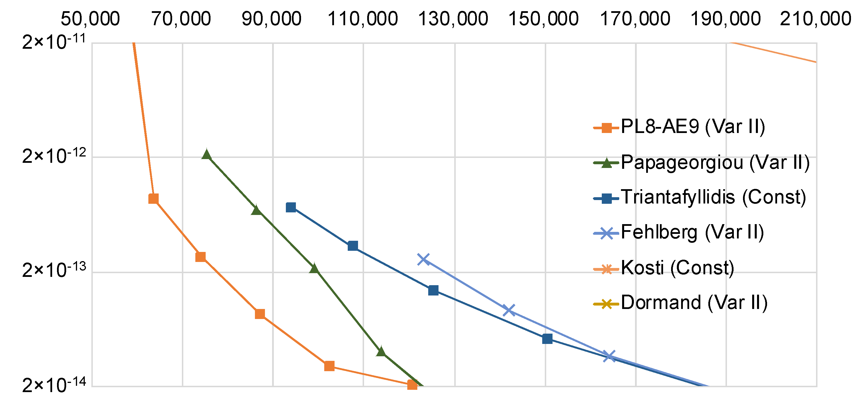
The efficiency of all compared methods in terms of the maximum absolute global norm error versus the function evaluations is presented in Figure 5 for $t\in [0,30\pi ]$. For each algorithm, the most efficient step size control is used, if applicable, which for all embedded pairs is the modified algorithm presented in Equation (10). Otherwise, a constant step is used.

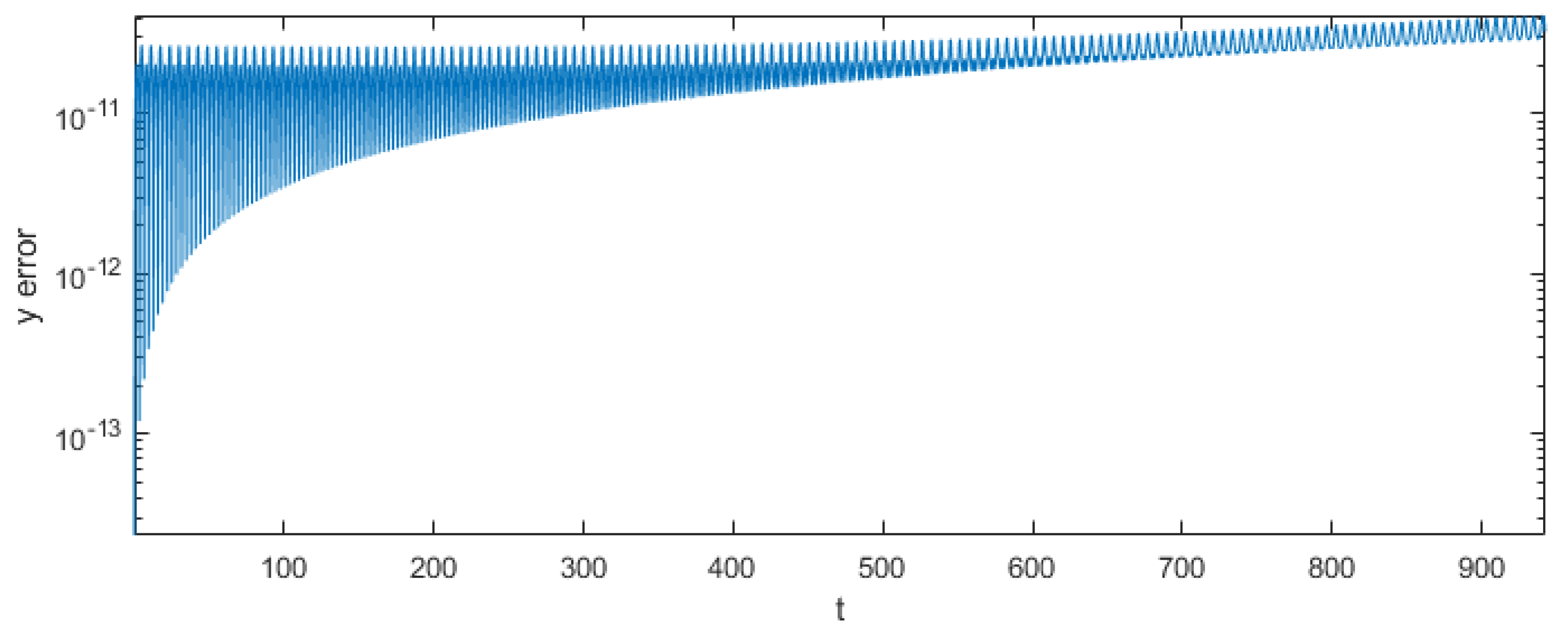
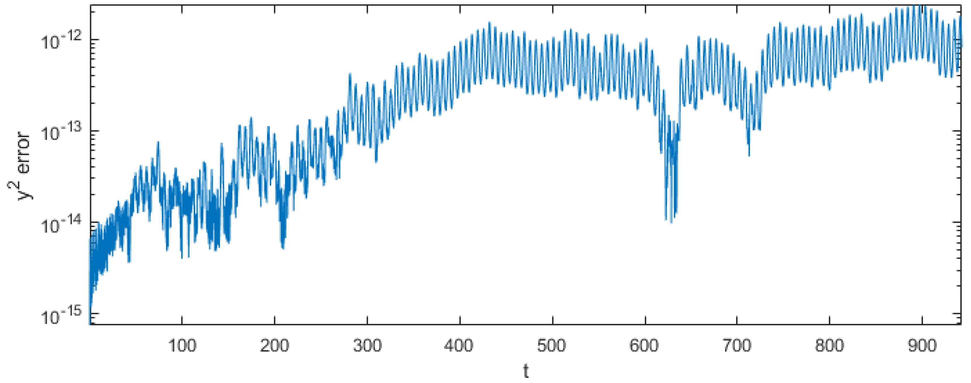
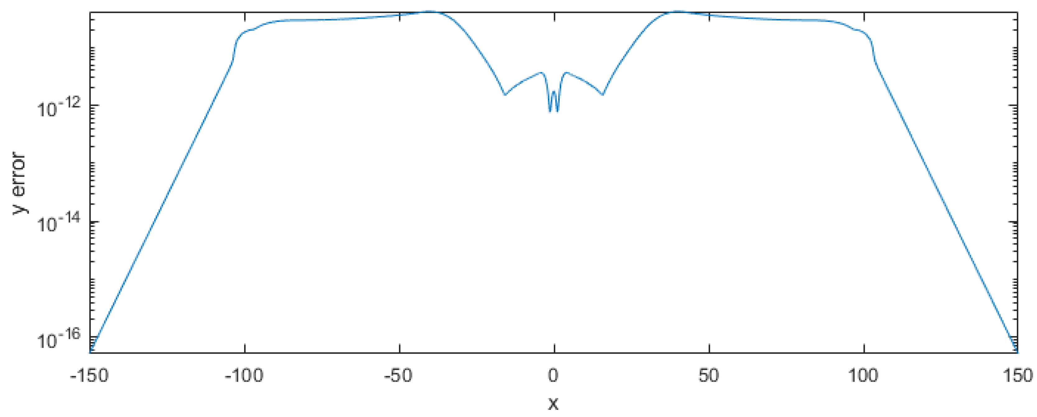
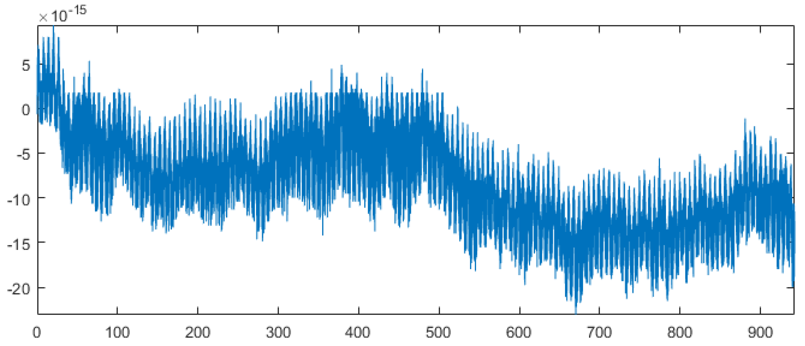
Furthermore, the maximum absolute error of the solution and of its square versus t are presented in Figure 6 and Figure 7 respectively, for $t\in [0,300\pi ]$. The maximum absolute error of the solution versus x is shown in Figure 8 and, finally, the error of the global norm is presented in Figure 9 and is measured by applying the Simpson rule on the conservation law, i.e., Equation (2), and evaluating the difference $E\left(\psi (x,t)\right)-E\left(\psi (x,0)\right)$.

6. Conclusions

We carefully selected a set of criteria for the construction of a new Runge–Kutta pair for the efficient computation of the nonlinear Schrödinger equation with varying coefficients. Then, from a plethora of solutions that satisfy the restrictions, we chose the one that optimises a set of properties in a way that follows the procedure of Section 3. Thus, we have developed an explicit 6(4)-order, eight-stage Runge–Kutta pair that has maximised phase-lag and amplification-error orders, for improved behaviour when solving the NLS with periodic/oscillatory solutions and constant coefficients, since the problem does not exhibit a dominant frequency. The stability characteristics were chosen so that the high-order method has a maximised real stability interval and that the low-order method has similar stability characteristics as the high-order one, to improve the local error estimation for extreme step sizes. Furthermore, the values of the RK coefficients have deliberately chosen to have similar orders of magnitude, to minimise the round-off error.

We compared the new RK method to other methods of the literature on a case of the NLS with a periodic-oscillatory solution. The numerical results verified the superiority of the new algorithm in terms of efficiency. The new method also presented a good behaviour of the maximum absolute error and the global norm in time, even after a high number of oscillations.

Additionally, we have developed a modified step size control algorithm, which was applied to the new pair as well as to other pairs of the literature. The results showed increased efficiency of all pairs included in the numerical experiments, compared to what the original step size control algorithm produced. The new RK pair was still the most efficient one among all pairs when using the modified step size control algorithm.

References

- Moloney, J.V.; Newell, A.C. Nonlinear optics. Phys. D Nonlinear Phenom. 1990, 44, 1–37. [Google Scholar] [CrossRef]
- Pitaevskii, L.; Stringari, S. Bose-Einstein Condensation; Oxford University Press: Oxford, UK, 2003. [Google Scholar]
- Malomed, B. Multi-Component Bose-Einstein Condensates: Theory. In Emergent Nonlinear Phenomena in Bose-Einstein Condensates: Theory and Experiment; Springer: Berlin/Heidelberg, Germany, 2008; pp. 287–305. [Google Scholar] [CrossRef]
- Hong, J.; Liu, Y. A novel numerical approach to simulating nonlinear Schrödinger equations with varying coefficients. Appl. Math. Lett. 2003, 16, 759–765. [Google Scholar] [CrossRef] [Green Version]
- Zhong, W.P.; Belić, M.; Zhang, Y. Second-order rogue wave breathers in the nonlinear Schrödinger equation with quadratic potential modulated by a spatially-varying diffraction coefficient. Opt. Express 2015, 23, 3708–3716. [Google Scholar] [CrossRef] [PubMed]
- Kengne, E. Analytical solutions of nonlinear Schrödinger equation with distributed coefficients. Chaos Solitons Fractals 2014, 61, 56–68. [Google Scholar] [CrossRef]
- Amador, G.; Colon, K.; Luna, N.; Mercado, G.; Pereira, E.; Suazo, E. On Solutions for Linear and Nonlinear Schrödinger Equations with Variable Coefficients: A Computational Approach. Symmetry 2016, 8, 38. [Google Scholar] [CrossRef] [Green Version]
- Obaidat, S.; Mesloub, S. A New Explicit Four-Step Symmetric Method for Solving Schrödinger’s Equation. Mathematics 2019, 7, 1124. [Google Scholar] [CrossRef] [Green Version]
- Benia, Y.; Ruggieri, M.; Scapellato, A. Exact Solutions for a Modified Schrödinger Equation. Mathematics 2019, 7, 908. [Google Scholar] [CrossRef] [Green Version]
- Polyanin, A.D. Comparison of the Effectiveness of Different Methods for Constructing Exact Solutions to Nonlinear PDEs. Generalizations and New Solutions. Mathematics 2019, 7, 386. [Google Scholar] [CrossRef] [Green Version]
- Chen, J.; Zhang, Q. Ground State Solution of Pohozaev Type for Quasilinear Schrödinger Equation Involving Critical Exponent in Orlicz Space. Mathematics 2019, 7, 779. [Google Scholar] [CrossRef] [Green Version]
- Tsitoura, F.; Anastassi, Z.A.; Marzuola, J.L.; Kevrekidis, P.G.; Frantzeskakis, D.J. Dark solitons near potential and nonlinearity steps. Phys. Rev. A 2016, 94, 063612. [Google Scholar] [CrossRef] [Green Version]
- Lyu, P.; Vong, S. A linearized and second-order unconditionally convergent scheme for coupled time fractional Klein-Gordon-Schrödinger equation. Numer. Methods Partial Differ. Equ. 2018, 34, 2153–2179. [Google Scholar] [CrossRef]
- Jiang, C.; Cai, W.; Wang, Y. Optimal error estimate of a conformal Fourier pseudo-spectral method for the damped nonlinear Schrödinger equation. Numer. Methods Partial Differ. Equ. 2018, 34, 1422–1454. [Google Scholar] [CrossRef]
- Liao, F.; Zhang, L.; Hu, X. Conservative finite difference methods for fractional Schrödinger–Boussinesq equations and convergence analysis. Numer. Methods Partial Differ. Equ. 2019, 35, 1305–1325. [Google Scholar] [CrossRef]
- Malomed, B.A.; Stepanyants, Y.A. The inverse problem for the Gross–Pitaevskii equation. Chaos 2010, 20, 013130. [Google Scholar] [CrossRef] [Green Version]
- Serkin, V.N.; Hasegawa, A. Novel Soliton Solutions of the Nonlinear Schrödinger Equation Model. Phys. Rev. Lett. 2000, 85, 4502–4505. [Google Scholar] [CrossRef]
- Tang, C.; Zhang, F.; Yan, H.Q.; Chen, Z.Q.; Luo, T. Three-Step Predictor-Corrector of Exponential Fitting Method for Nonlinear Schrödinger Equations. Commun. Theor. Phys. 2005, 44, 435–439. [Google Scholar] [CrossRef]
- Kosti, A.A.; Anastassi, Z.A.; Simos, T.E. Construction of an optimized explicit Runge–Kutta–Nyström method for the numerical solution of oscillatory initial value problems. Comput. Math. Appl. 2011, 61, 3381–3390. [Google Scholar] [CrossRef] [Green Version]
- Kosti, A.A.; Anastassi, Z.A.; Simos, T.E. An optimized explicit Runge–Kutta–Nyström method for the numerical solution of orbital and related periodical initial value problems. Comput. Phys. Commun. 2012, 183, 470–479. [Google Scholar] [CrossRef]
- Anastassi, Z.A.; Kosti, A.A. A 6(4) optimized embedded Runge–Kutta–Nyström pair for the numerical solution of periodic problems. J. Comput. Appl. Math. 2015, 275, 311–320. [Google Scholar] [CrossRef]
- Kosti, A.A.; Anastassi, Z.A. Explicit almost P-stable Runge–Kutta–Nyström methods for the numerical solution of the two-body problem. Comput. Appl. Math. 2015, 34, 647–659. [Google Scholar] [CrossRef]
- Demba, M.; Senu, N.; Ismail, F. A 5(4) Embedded Pair of Explicit Trigonometrically-Fitted Runge–Kutta–Nyström Methods for the Numerical Solution of Oscillatory Initial Value Problems. Math. Comput. Appl. 2016, 21, 46. [Google Scholar] [CrossRef] [Green Version]
- Ahmad, N.A.; Senu, N.; Ismail, F. Phase-Fitted and Amplification-Fitted Higher Order Two-Derivative Runge-Kutta Method for the Numerical Solution of Orbital and Related Periodical IVPs. Math. Probl. Eng. 2017, 2017, 1871278. [Google Scholar] [CrossRef]
- Simos, T.E.; Papakaliatakis, G. Modified Runge–Kutta Verner methods for the numerical solution of initial and boundary-value problems with engineering applications. Appl. Math. Model. 1998, 22, 657–670. [Google Scholar] [CrossRef]
- Tsitouras, C.; Simos, T.E. Optimized Runge–Kutta pairs for problems with oscillating solutions. J. Comput. Appl. Math. 2002, 147, 397–409. [Google Scholar] [CrossRef] [Green Version]
- Triantafyllidis, T.V.; Anastassi, Z.A.; Simos, T.E. Two optimized Runge-Kutta methods for the solution of the Schrödinger equation. MATCH Commun. Math. Comput. Chem. 2008, 60, 3. [Google Scholar]
- Kosti, A.A.; Anastassi, Z.A.; Simos, T.E. An optimized explicit Runge-Kutta method with increased phase-lag order for the numerical solution of the Schrödinger equation and related problems. J. Math. Chem. 2010, 47, 315. [Google Scholar] [CrossRef]
- Papageorgiou, G.; Tsitouras, C.; Papakostas, S.N. Runge-Kutta pairs for periodic initial value problems. Computing 1993, 51, 151–163. [Google Scholar] [CrossRef]
- Berland, J.; Bogey, C.; Bailly, C. Low-dissipation and low-dispersion fourth-order Runge–Kutta algorithm. Comput. Fluids 2006, 35, 1459–1463. [Google Scholar] [CrossRef]
- Tsitouras, C. A parameter study of explicit Runge-Kutta pairs of orders 6(5). Appl. Math. Lett. 1998, 11, 65–69. [Google Scholar] [CrossRef] [Green Version]
- Shampine, L.F. Error estimation and control for ODEs. J. Sci. Comput. 2005, 25, 3–16. [Google Scholar] [CrossRef]
- Auzinger, W.; Kassebacher, T.; Koch, O.; Thalhammer, M. Adaptive splitting methods for nonlinear Schrödinger equations in the semiclassical regime. Numer. Alg. 2016, 72, 1–35. [Google Scholar] [CrossRef] [Green Version]
- Auzinger, W.; Hofstätter, H.; Koch, O.; Thalhammer, M. Defect-Based Local Error Estimators for Splitting Methods, with Application to Schrödinger Equations, Part III. J. Comput. Appl. Math. 2015, 273, 182–204. [Google Scholar] [CrossRef]
- Thalhammer, M.; Abhau, J. A numerical study of adaptive space and time discretisations for Gross–Pitaevskii equations. J. Comput. Phys. 2012, 231, 6665–6681. [Google Scholar] [CrossRef] [PubMed] [Green Version]
- Balac, S.; Fernandez, A. Mathematical analysis of adaptive step-size techniques when solving the nonlinear Schrödinger equation for simulating light-wave propagation in optical fibers. Opt. Commun. 2014, 329, 1–9. [Google Scholar] [CrossRef] [Green Version]
- Butcher, J.C. Trees and numerical methods for ordinary differential equations. Numer. Alg. 2010, 53, 153–170. [Google Scholar] [CrossRef]
- Popelier, P.L.; Simos, T.E.; Wilson, S. Chemical Modelling: Applications and Theory; Royal Society of Chemistry: London, UK, 2000; Volume 1. [Google Scholar]
Figure 1.
Real part , showing different frequencies for various values of x.
Figure 2.
Stability regions of both high-order and low-order methods of the new Runge–Kutta (RK) pair of Table 1.
Figure 3.
Numerical solution of versus x and t.
Figure 4.
Maximum absolute global norm error versus the function evaluations for the pairs PL8-AE9 (Table 1) (■), Papageorgiou et al. [29] (●) and Fehlberg [37] (▲). For each of the three pairs, Var II (solid line —) denotes the modified step size control algorithm described with Equation (10), while Var I (dashed line – –) denotes the original method in Equation (7).
Figure 5.
Maximum absolute global norm error versus the function evaluations for all compared methods in Table 2.
Figure 6.
The maximum absolute error of the solution versus t.
Figure 7.
The maximum absolute error of the square of the solution versus t.
Figure 8.
The maximum absolute error of the solution versus x.
Figure 9.
The global norm error versus t.