Analysis of Queueing System MMPP/M/K/K with Delayed Feedback

Abstract

The model of multi-channel queuing system with Markov modulated Poisson process (MMPP) flow and delayed feedback is considered. After the customer is served completely, they will decide either to join the retrial group again for another service (feedback) with some state-dependent probability or to leave the system forever with complimentary probability. Feedback calls organize an orbit of repeated calls (r-calls). If upon arrival of an r-call all the channels of the system are busy, then it either leaves the system with some state-dependent probability or with a complementary probability returns to orbit. Methods to calculate the steady-state probabilities of the appropriate three-dimensional Markov chain as well as performance measures of investigated system are developed. Results of numerical experiments are demonstrated.

1. Introduction

Most of the papers on queuing theory have considered the systems without feedback, i.e. without re-service phenomena. However, queues with feedback occur in many practical situations, e.g., multiple access telecommunication systems, where data that is transmitted erroneously are sent again can be modeled as queue with feedback.

We will distinguish between re-service of two types: instantaneous and delayed re-service. In the case of instantaneous repetition, after completion of the previous service, the customer either requires re-service immediately with some positive probability or leaves the system forever with complimentary probability. In the case of delayed re-service, after the customer is served completely, they will decide either to join the retrial group again for another service with some positive probability or to leave the system forever with complimentary probability. Such kinds of feedbacks are called Bernoulli feedback.

Pioneer works related to queuing systems with feedbacks of both types were Takacs’s papers [1,2]. Note that the model of the queuing system with instantaneous feedback (IFB) was investigated in Reference [1], while in Reference [2] the model of the queuing system with delayed feedback (DFB) was considered. In both papers, the method of generating functions was used.

In the last three decades, various authors have intensively studied models of queuing systems with feedback of both types. In this paper, we investigated the model of the queuing system with DFB. A detailed review of a large number of publications in that direction can be found in Reference [3]. Therefore, we have provided a quick review of the work which is not included in Reference [3] below.

Ayyapan et al. considered M/M/1 retrial queuing systems with loss and with DFB under non-pre-emptive [4] and pre-emptive [5] priority service disciplines. Two types of customers arrive and the retrial, loss and feedback is allowed for low priority customers only. If the server is free at the time of the arrival of low priority customer, then an incoming customer immediately begins to be serviced. After completion of service, the low priority customer either may re-join the orbit of infinite size or leaves the system. If the server is busy then the low priority arriving customer either goes to orbit or becomes a source of repeated calls. If the server is free at the time of the arrival of high priority customer, then the arriving call begins to be served immediately and high priority customer leaves the system after service completion. In Reference [4] the non-pre-emptive priority service discipline is used, i.e., if the server is engaging with a low priority customer and the higher priority customer comes then the high priority customer will get service only after completion of the service of the low priority customer who is in service. In Reference [5] the pre-emptive priority service is used, i.e., if the server is engaging with low priority customer and the higher priority customer enters then the high priority customer will get service immediately and the low priority customer who is in service goes to orbit without completion of his service. In both papers, matrix geometric method by Neuts [6] is used.

Belarbi et al. [7] focuses on an M/M/1/N < ∝ retrial queuing systems with single flow, loss and with two orbits for DFB. If upon arrival, the customers find the queue full, then they decide to stay for an attempt to get service or leave the system. Arriving customers who decide to stay for an attempt have to choose one of the orbits in accordance with the probabilities that depend on thresholds in orbits. After the customer is served completely, they may decide to either attempt for re-service (feedback) or leave the system forever. In this case, the selection of one of the orbits occurs according to the Bernoulli scheme. In Reference [7] the generating functions method is used.

Choi et al. [8] investigated an M/M/c/c retrial queues with geometric loss and with DFB when c = 1, 2. An arriving customer is served immediately if one of the servers is idle, and if all servers are busy, they will either join the retrial group to try again after a random amount of time or leave the system forever without service. On retrials, each customer is treated the same as a primary customer. If the retrial customer finds free servers, they receive service immediately, and if all the servers are busy, they will either leave the system forever or join the retrial group. All customers in the retrial group act independently of each other. The retrial time is exponentially distributed with finite mean and is independent of all previous retrial times and all other stochastic processes in the system. After the customer is served completely, they will decide either to join the retrial group again for another service (feedback) or to leave the system forever. They found the joint generating function of the number of busy servers and the number of customers in the retrial group by solving Kummer differential equation for c = 1, and by the method of series solution for c = 1, 2.

Kumar et al. [9] considered an M/M/c/N + c queue with DFB and with constant retrial rate, which is independent of the number of customers in the retrial group. Note that a customer in the orbit can enter the service facility at the retrial instant only when there are idle servers. The problem is solved by the matrix-geometric method [6]. The same model was investigated in Reference [10] by Do where an efficient algorithm based on spectral expansion method by Mitrani and Chakka [11] is developed.

In Reference [12] Mokaddis et al. considered M/G/1 retrial DFB queue without a waiting space and single vacation where the server is subjected to starting failures. It is assumed that the retrial time is governed by an arbitrary distribution and that only the customer at the head of the orbit queue is allowed access to the server. The server leaves for a vacation as soon as the system becomes empty. When the server returns from the vacation and finds no customers, it waits free for the first customer to arrive from outside the system. If the server is started successfully (with a certain probability), the customer gets service immediately. Otherwise, the repair for the server starts immediately and the customer must leave for the orbit and make a retrial later. The system size distribution at random points and various performance measures are derived.

It is important to note that in the works indicated above it is assumed that the departure and feedback probabilities are constant quantities, i.e., they do not depend on the state of the system. This assumption significantly limits the application areas of the proposed models, since decisions about going into orbit or leaving orbit without getting re-service often depend on the current state of the system.

In the literature, models of queuing systems with DFB under variable input flow intensity have not been studied. Based on this, in the present paper, we studied models of queuing systems with DFB in the presence of a Markov modulated Poisson process (MMPP) [13] in which the departure and feedback probabilities depended on the current state of the system. Recently a similar model by using the asymptotic method was studied in Reference [14].

This paper is structured as follows. The mathematical model of the investigated system is described in Section 2. The generator matrix of the three-dimensional Markov chain (3D MC) is created in Section 3. Here the exact method to calculate the steady-state probabilities of the constructed 3D MC is indicated and explicit formulas for some performance measures of the investigated system is developed as well. In Section 4, an approximate method for solving indicated above problems is proposed. Results of numerical experiments that show high accuracy of the approximate method are demonstrated in Section 5. Conclusions are given in Section 6.

2. Mathematical Model

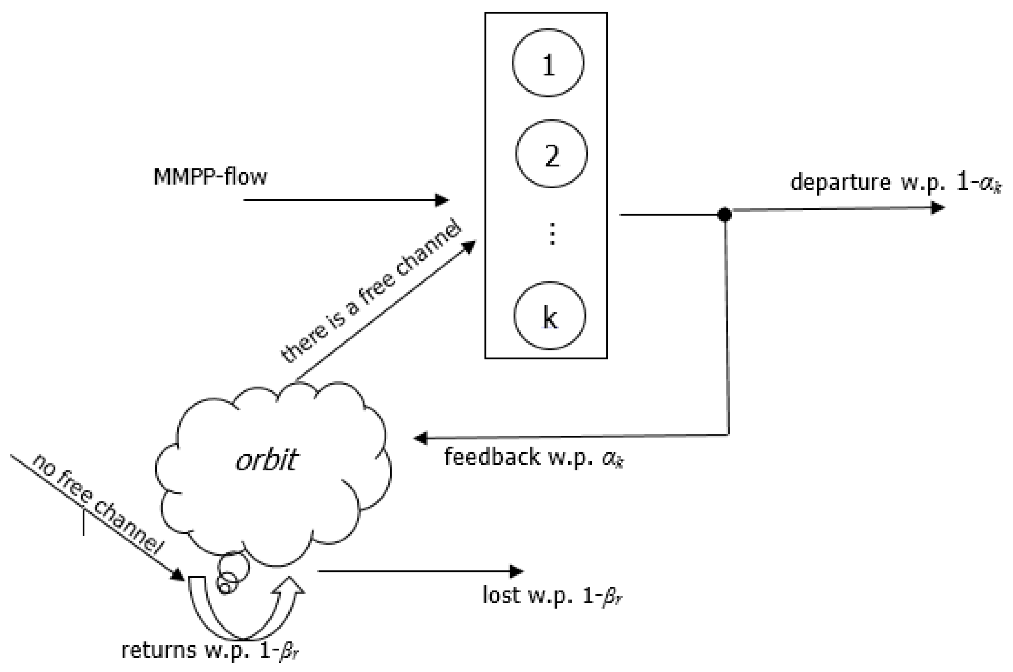
Pictorial representation of the investigated system is shown in Figure 1.

The system contains $K>1$ identical channels and incoming calls form the MMPP-flow. The Markov chain (MC), which controls the intensities of the incoming flow, has a generating matrix (GM) $\Sigma =\Vert {\sigma }_{ij}\Vert$ of dimension $N\times N$, where ${\sigma }_{ij}$ determines the transition intensity from state $i$ to state $j$, $i,j=1,2,\dots ,N$, and ${\sigma }_{ii}=-{\displaystyle \sum _{j=1,j\ne i}^N{\sigma }_{ij}}$.

It is assumed that when control MC is in a state $n$, the intensity of the incoming stream is equal ${\lambda }_n,n=1,2,\dots ,N$, and when the state of the control MC changes, the intensity of the incoming flow also changes instantly. The vector of intensities of the incoming flow is denoted by $\lambda =\left({\lambda }_1,{\lambda }_2,\dots ,{\lambda }_N\right)$.

Arriving from outside calls is called a primary call (p-call). An incoming call is accepted for service if at that moment there is a free channel; otherwise, i.e., if at that moment all channels are busy, then the incoming call is lost with a probability (w.p.) of one. After completion of the service process, the call, according to the Bernoulli scheme, either w.p. ${\alpha }_k$ requires repeated service, or with a complementary probability leaves the system. The departure and feedback probabilities depend on a parameter $k$ that indicates the number of occupied channels immediately before the moment of a call’s departure, and it is assumed that ${\alpha }_k>0$ for at least one $k,k=1,2,\dots ,K.$

Feedback calls organize an orbit of repeated calls (r-calls) with a finite size $R,0<R<\infty$, i.e., a feedback call is accepted into orbit if the total number of r-calls is less than $R$; otherwise, a feedback call leaves the system w.p. 1.

Service times for both types of calls are independent and identically distributed (i.i.d.) random variables (r.v.) and suppose that their distribution function is an exponential one with a common average $1/\mu$.

Calls from orbit come through random times that obey the exponential distribution with the mean $1/\eta .$ If upon arrival of an r-call all the channels of the system are busy, then it leaves the system w.p. ${\beta }_r,$ and with a complementary probability $1-{\beta }_r$ returns to orbit, where $r$ means the current number of calls in orbit, $r=1,2,\dots ,R.$ It is assumed that the random processes of changing the states of the MC, which control the intensity of the incoming flow, service of calls and the arriving of r-calls from orbit, are independent of each other.

The problem is to determine the stationary distribution of states of a given system. The solution to this problem allows us to find the performance measures of the system under study: the average number of busy channels $(K_{av})$, the average number of repeated calls in orbit $(L_0)$, as well as the probability that all channels of the system are busy $(CBP)$.

3. Method Based on Balance Equations

The state of the system at an arbitrary moment of the time is defined by the three-dimensional vector $(n,k,r)$, where $n$ is the state of the MMPP-flow, $k$ is total number of busy channels and $r$ is number of retrial calls in orbit. Taking into account the type of distribution functions of all r.v. that are involved in the formation of the model we conclude that the state space of the investigated system is determined as follows:

$$E=\left\{1,2,\dots ,N\right\}\times \left\{0,1,\dots ,K\right\}\times \left\{0,1,\dots ,R\right\}.$$

(1)

Transition intensity from state $(n,k,r)$ to state $(n^{\prime },k^{\prime },r^{\prime })$ is denoted by $q((n,k,r),(n^{\prime },k^{\prime },r^{\prime }))$. These quantities are determined as follows:

• The transition $(n,k,r)\to \left(n^{\prime },k,r\right),n^{\prime }\ne n$ is carried out with intensity ${\sigma }_{n,n^{\prime }}$ when the state of the MMPP flow changes;
• The transition $(n,k,r)\to \left(n,k+1,r\right),k<K,$ is carried out with intensity ${\lambda }_n$ upon receipt of the p-call;
• The transition $(n,k,r)\to \left(n,k-1,r\right),k>0,r<R,$ is carried out with intensity $k\mu \left(1-{\alpha }_k\right)$ upon completion of the call service and having left the system;
• The transition $(n,k,r)\to \left(n,k-1,r+1\right),k>0,r<R,$ is carried out with intensity $k\mu {\alpha }_k$ upon completion of the call service and its departure into orbit;
• The transition $(n,k,R)\to \left(n,k-1,R\right),k>0,$ is carried out with intensity $k\mu$ upon completion of the call service;
• The transition $(n,k,r)\to \left(n,k+1,r-1\right),k<K,r>0,$ is carried out with intensity $r\eta$ upon receipt of an r-call from orbit;
• The transition $(n,K,r)\to \left(n,K,r-1\right),r>0,$ is carried out with intensity $r\eta {\beta }_r$ when r-call is lost from orbit.

Therefore, the positive elements of GM of the investigated 3D MC are determined as follows:

$$q\left(\left(n,k,r\right),\left(n^{\prime },k^{\prime },r^{\prime }\right)\right)=\{\begin{array}{ll}{\sigma }_{n{n}^{\prime }},\hfill & n^{\prime }\ne n,k^{\prime }=k,r^{\prime }=r,\hfill \\ {\lambda }_n,\hfill & n^{\prime }=n,k^{\prime }=k+1,r^{\prime }=r,\hfill \\ k\mu \left(1-{\alpha }_k\right),\hfill & k>0,r<R,n^{\prime }=n,k^{\prime }=k-1,r^{\prime }=r,\hfill \\ k\mu {\alpha }_k,\hfill & k>0,r<R,n^{\prime }=n,k^{\prime }=k-1,r^{\prime }=r+1,\hfill \\ k\mu ,\hfill & k>0,r=R,n^{\prime }=n,k^{\prime }=k-1,r^{\prime }=r,\hfill \\ r\eta ,\hfill & k<K,r>0,n^{\prime }=n,k^{\prime }=k+1,r^{\prime }=r-1,\hfill \\ r\eta {\beta }_r,\hfill & k=K,r>0,n^{\prime }=n,k^{\prime }=k,r^{\prime }=r-1.\hfill \end{array}$$

(2)

From relations in Equation (2) we conclude that the investigated 3D MC with state space in Equation (1) is irreducible, i.e., in this chain there exist steady-state probabilities. Let $p(n,k,r)$ denote steady-state probability of state $(n,k,r)\in E.$ These probabilities satisfy the system of equilibrium equations (SEE), which are compiled using relations in Equation (2). The explicit form of this SEE is not given here due to the obviousness of its derivation and cumbersome nature.

Finding the steady-state probabilities allows us to calculate the performance measures of the system under study. So, the average number of busy channels and the average number of r-calls in orbit are determined as the mathematical expectations of the corresponding r.v., i.e.,

$$K_{av}={\displaystyle \sum _{n=1}^N{\displaystyle \sum _{k=1}^{K}k{\displaystyle \sum _{r=0}^{R}p\left(n,k,r\right)}}};$$

(3)

$$L_o={\displaystyle \sum _{n=1}^N{\displaystyle \sum _{r=1}^{R}r{\displaystyle \sum _{k=0}^{K}p\left(n,k,r\right)}}}.$$

(4)

The probability that all channels of the system are busy is determined as follows:

$$CBP={\displaystyle \sum _{\left(n,K,r\right)\in E}p\left(n,K,r\right)}.$$

(5)

Note that, due to the complex structure of the obtained GM (see Equation (2)), it is not possible to find an analytical solution to the corresponding SEE for steady-state probabilities. Therefore, to solve it, one has to use numerical methods of linear algebra, and modern software packages allow us to solve SEE of moderate dimension (see References [15,16]). However, for models of large dimensions, these methods will require a huge runtime, and often suffer from computational instability. Based on this, an alternative (approximate) method for solving this problem is given below. It is based on the hierarchical space merging approach for multidimensional MCs [17].

4. Method Based on Space Merging Hierarchy

For the correct application of the developed method, we assume that the MMPP flow is inertial. This means that transitions between its states occur with low intensities. When fulfilling this assumption, we consider the following splitting of the state space from Equation (1):

$$E={\displaystyle \underset{n=1}{\overset{N}{\cup }}{E}_n},E_n{\displaystyle \cap E_{n^{\prime }}=\varnothing ,n\ne n^{\prime },}$$

(6)

where $E_n=\left\{\left(n,k,r\right)\in E:k=0,1,\dots ,K;r=0,1,\dots ,R\right\},n=1,2,\dots ,N.$

Based on splitting Equation (6) in the state space of Equation (1), the following merge function is defined:

$$U_1\left(n,k,r\right)=<n>,\left(n,k,r\right)\in E_n,$$

(7)

where $<n>$ is the merged state which includes all states from the class $E_n$, $n=1,2,\dots ,N$. We denote ${\Omega }_1=\left\{<n>:n=1,2,\dots ,N\right\}.$

The steady-state probabilities of the initial 3D MC are determined as follows (see [17]):

$$p\left(n,k,r\right)\approx {\rho }_n\left(k,r\right){\pi }_1\left(<n>\right),$$

(8)

where ${\rho }_n\left(k,r\right)$ is the probability of state $(k,r)$ within splitting model with state space $E_n$, ${\pi }_1\left(<n>\right)$ is the probability of merged state $<n>\in \Omega {}_1.$

From Equation (8) we conclude that to calculate the steady-state probabilities of the initial 3D MC, it is necessary to find the state probabilities of the 2D MCs (their number is equal $N$) and one 1D MC.

The transitions between the states of the Markov chain, which control the intensity of the incoming flow, do not depend on the status of channels (busy or free) and on the intensity of r-calls. Therefore, its stationary distribution ${\pi }_1\left(<n>\right),<n>\in {\Omega }_1$ is uniquely determined using its generating matrix $\Sigma .$ In other words, to solve the problem, it is enough to find the stationary distribution of 2D MCs with state spaces $E_n,n=1,2,\dots ,N.$

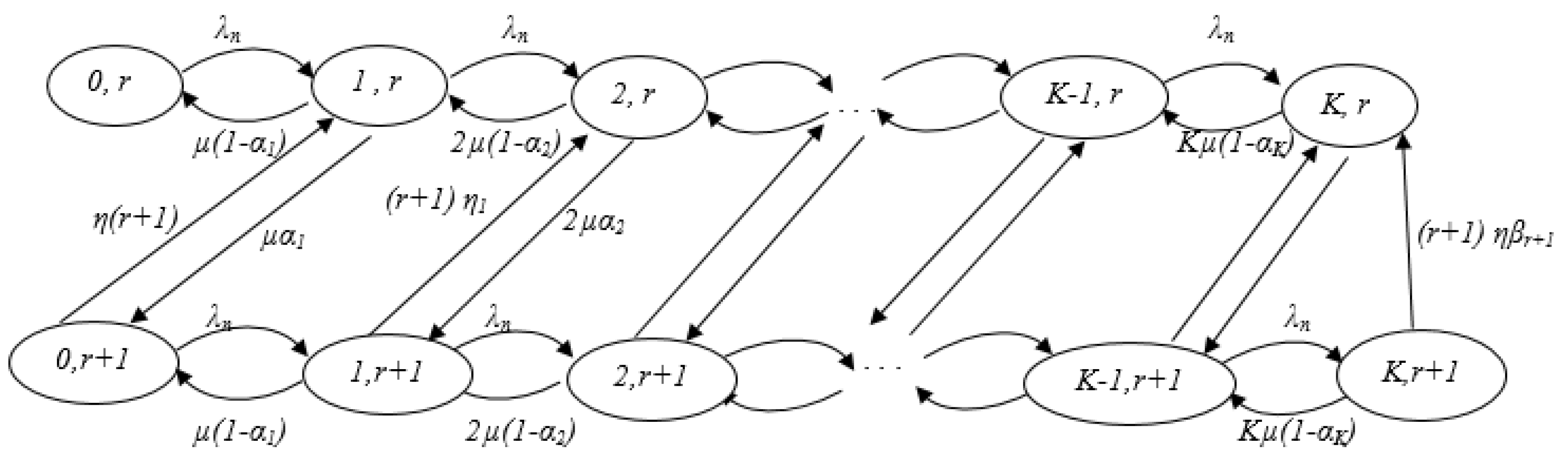
A fragment of the transition graph between the states of a split model with a state space $E_n$ is shown in Figure 2.

Computational difficulties arise in solving the latter problem if the number of channels and the size of the orbit are huge. Therefore, the merge procedure (second level of the hierarchy) is applied to these 2D MCs. Since all splitting models are identical, we fix the value of parameter $n$ and consider the split model with the state space $E_n.$

For correct application of the proposed method, it is assumed that $\min \left\{{\lambda }_n:n=1,2,\dots ,N\right\}>>\eta$. Under this assumption consider following splitting in class $E_n$:

$$E_n={\displaystyle \underset{r=0}{\overset{R}{\cup }}{E}_n^r},E_n^r{\displaystyle \cap E_n^{r^{\prime }}=\varnothing ,r\ne r^{\prime },}$$

(9)

where $E_n^r=\left\{\left(k,r\right)\in E_n:k=0,1,\dots ,K\right\},r=0,1,\dots ,R.$

As above (see Equation (7)), based on splitting Equation (9) in the state space $E_n$ the following merge function is defined:

$$U_2\left(\left(k,r\right)\right)=<r>,\left(k,r\right)\in E_n^r,$$

where $<r>$ is the merge state which includes all states from the class $E_n^r$. We denote ${\Omega }_2=\left\{<r>:r=0,1,\dots ,R\right\}.$

In accordance [17] we have:

$${\rho }_n\left(k,r\right)\approx {\rho }_n^r\left(k\right){\pi }_2^n\left(<r>\right),$$

(10)

where ${\rho }_n^r\left(k\right)$ is the probability of state $(k,r)$ within the splitting model with space $E_n^r$, ${\pi }_2^n\left(<r>\right)$ is the probability of the merged state $<r>\in {\Omega }_2.$

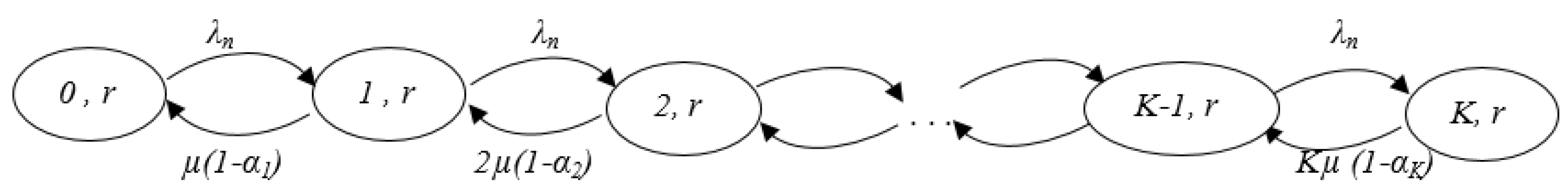
The transition graph between the states of a split model with a state space $E_n^r,r=0,1,\dots ,R-1,$ is shown in Figure 3.

In a class $E_n^r,r=0,1,\dots ,R,$ in a state vector, the second component is constant and equal $r$. Therefore, in a splitting model with space $E_n^r$ each state $(k,r)$ can be specified only by the first component, i.e., hereinafter state $(k,r)\in E_n^r$ referred to as $k,k=0,1,\dots ,K$. Then from relations in Equation (2) we conclude that the intensities of transitions between the states of the splitting model with space $E_n^r,r=0,1,\dots ,R-1,$ are independent of the parameter $r$, and are determined as follows (see Figure 3):

$$q_n\left(k,k^{\prime }\right)=\{\begin{array}{ll}{\lambda }_n,\hfill & \mathrm{if}{k}^{\prime }=k+1,\hfill \\ k\mu \left(1-{\alpha }_k\right),\hfill & \mathrm{if}{k}^{\prime }=k-1.\hfill \end{array}$$

(11)

From Equation (11) we conclude that the probabilities of the states of splitting models with space $E_n^r,r=0,1,\dots ,R-1,$ coincide with the state probabilities of the one-dimensional birth–death process in which the birth intensity is equal to ${\lambda }_n$ and the death intensity in the state $k$ is equal to $k\mu \left(1-{\alpha }_k\right),k=1,\dots ,K.$ For a splitting model with a space $E_n^R$, the intensities of transitions between its states are determined similarly to Reference (11), but in this model, on the right side of the indicated formulae (in the second line), the term $1-{\alpha }_k$ is replaced by 1. This is because if the call arrives at the moment when the orbit is completely full then it is lost w.p. 1. Therefore, the state probabilities of the splitting model with space $E_n^R$ coincide with the probabilities of the Erlang’s M/M/K/K system with a load ${\nu }_n$.

After certain mathematical transformations, we obtain that the intensities of transitions between states of space ${\Omega }_2$ are determined as follows:

$$q_n\left(<r>,<r^{\prime }>\right)=\{\begin{array}{ll}{\Lambda }_n,\hfill & \mathrm{if}{r}^{\prime }=r+1,\hfill \\ r{\Psi }_r\left(n\right),\hfill & \mathrm{if}{r}^{\prime }=r-1,\hfill \end{array}$$

(12)

where ${\Lambda }_n=\mu {\displaystyle \sum _{k=1}^{K}k{\alpha }_k{\rho }_n^r\left(k\right)},{\Psi }_r\left(n\right)=\eta \left(1-\left(1-{\beta }_r\right){\rho }_n^r\left(K\right)\right).$

Therefore, from relations in Equation (12) we conclude that the probabilities of merged states are calculated as follows:

$${\pi }_2^n\left(<r>\right)=\frac{{\Lambda }_n^r}{r!{\displaystyle \prod _{i=1}^r{\Psi }_i\left(n\right)}}{\pi }_2^n\left(<0>\right),r=1,\dots ,R,$$

(13)

where ${\pi }_2^n\left(<0>\right)$ is found from normalizing condition, i.e., ${\displaystyle \sum _{r=0}^R{\pi }_2^n\left(<r>\right)}=1.$

Finally, taking into account relations from Equations (8), (10), (11) and (13), approximate values of the steady-state of the initial 3D MC are found. Further, after certain mathematical transformations, we obtain the following approximate formulas for calculating the performance measures of the system under study:

$$K_{av}\approx {\displaystyle \sum _{n=1}^N{\pi }_1\left(<n>\right){\displaystyle \sum _{k=1}^{K}k{\displaystyle \sum _{r=0}^R{\rho }_n^r\left(k\right){\pi }_2^n\left(<r>\right)}}};$$

(14)

$$L_o\approx {\displaystyle \sum _{n=1}^N{\pi }_1\left(<n>\right){\displaystyle \sum _{r=1}^{R}r{\pi }_2^n\left(<r>\right)}};$$

(15)

$$CBP\approx {\displaystyle \sum _{n=1}^N{\pi }_1\left(<n>\right){\displaystyle \sum _{r=0}^R{\rho }_n^r\left(K\right){\pi }_2^n\left(<r>\right)}}.$$

(16)

Special cases. Note that in the cases ${\alpha }_k=\alpha$ for all $k=1,2,\dots ,K$, and ${\beta }_r=\beta$ for all $r=1,2,\dots ,R$, the Equations (11–16) are even more simplified. Moreover, in this case it is possible to obtain explicit solutions for models with an infinite number of channels and/or an infinite orbit size.

So, for a model with a finite number of channels $\left(K<\infty \right)$ and an infinite orbit size $\left(R=\infty \right)$, the state probabilities inside all splitting models with space $E_n^r,r=0,1,2,\dots ,$ coincide with the state probabilities of the Erlang model M/M/K/K with load ${\nu }_n/\left(1-\alpha \right)$. The probabilities of merged states coincide with the probabilities of the states of the model M/M/∞ with the load ${\tilde{\theta }}_n={\tilde{\Lambda }}_n/\tilde{\Psi }\left(n\right)$, i.e.,

$${\pi }_2^n\left(<r>\right)=\frac{{\tilde{\theta }}_n^r}{r!}\exp \left(-{\tilde{\theta }}_n\right),r=0,1,2,\dots ,$$

where ${\tilde{\Lambda }}_n=\mu \alpha B_{av}\left(\frac{{\nu }_n}{1-\alpha },K\right),\tilde{\Psi }\left(n\right)=\eta \left(1-\left(1-\beta \right)E_B\left(\frac{{\nu }_n}{1-\alpha },K\right)\right)$.

Hereinafter, $E_B\left(x,K\right)$ and $B_{av}\left(x,K\right)$ denote the Erlang B-formula and the average number of busy channels for the M/M/K/K system with a load $x$, respectively, i.e.,

$$E_B\left(x,K\right)=\frac{x^K}{K!}/{\displaystyle \sum _{k=0}^K\frac{x^k}{k!}};B_{av}\left(x,K\right)=x\left(1-E_B\left(x,K\right)\right).$$

Then from Equations (14)–(16) we obtain that the performance measures of this model are determined as follows:

$$\begin{gathered} K_{av}\approx {\displaystyle \sum _{n=1}^N{\pi }_1\left(<n>\right)B_{av}\left(\frac{{\nu }_n}{1-\alpha },K\right)}; \\ {L}_o\approx {\displaystyle \sum _{n=1}^N{\pi }_1\left(<n>\right)}{\tilde{\theta }}_n; \\ CBP\approx {\displaystyle \sum _{n=1}^N{\pi }_1\left(<n>\right)E_B\left(\frac{{\nu }_n}{1-\alpha },K\right)}. \end{gathered}$$

In a model with an infinite number of channels $\left(K=\infty \right)$ and an infinite orbit size $\left(R=\infty \right)$, the state probabilities inside all split models with space $E_n^r,r=0,1,2,\dots ,$ coincide with the state probabilities of the model M/M/∞ with a load ${\nu }_n/\left(1-\alpha \right)$; the probabilities of merged states ${\pi }_2^n\left(<r>\right),r=0,1,2,\dots$, coincide with the probabilities of the states of the model M/M/∞ with a load ${\widehat{\theta }}_n={\widehat{\Lambda }}_n/\eta$, where ${\widehat{\Lambda }}_n=\mu {\nu }_n\frac{\alpha }{1-\alpha }$. In this model, we have $CBP=0$, however the remaining performance measures are defined as follows:

$$K_{av}\approx \frac{1}{1-\alpha }{\displaystyle \sum _{n=1}^N{\pi }_1\left(<n>\right){\nu }_n};L_o\approx {\displaystyle \sum _{n=1}^N{\pi }_1\left(<n>\right)}{\widehat{\theta }}_n.$$

5. Numerical Results

Here we present the results of numerical experiments. These experiments had two goals: (1) investigation of the accuracy of the developed approximate method; (2) investigation of the behavior of the performance measures versus both the feedback ${\alpha }_k,k=1,\dots ,K$ and retrial probabilities ${\beta }_r,r=1,\dots ,R$.

Exact values of the steady-state probabilities were calculated from the corresponding SEE and the accuracy of their calculation might be estimated using various similarity norms. For this purpose, the cosine similarity norm was used, since in our experiments it estimated not only the orientation of the steady-state probability vectors in various (exact and approximate) approaches, as well as their Euclidean proximity. This is because, according to the normalization condition, the ends of these vectors were in the same hyper plane of the Euclidean space of dimension $N\left(K+1\right)\left(R+1\right)$.

For the sake of clarity, let us assume that the MMPP flow is determined using a MC with three states (i.e., $N=3$) and the following generating matrix:

$$\Sigma =\Vert \begin{array}{lll}-35\hfill & 15\hfill & 20\hfill \\ 15\hfill & -25\hfill & 10\hfill \\ 10\hfill & 10\hfill & -20\hfill \end{array}\Vert .$$

The vector of intensities of the incoming flow is defined as follows: $\lambda =\left(20,30,40\right)$; rate of feedback calls from orbit is $\eta =15$. It is assumed that the parameters ${\alpha }_k,k=1,\dots ,K$, and ${\beta }_r,r=1,\dots ,R$, are constant, i.e., ${\alpha }_k=\alpha =0.2,{\beta }_r=\beta =0.9$.

The results of the corresponding numerical experiments are shown in

Table 1. Results of numerical experiments, EV—exact values, AV—approximate values.

$\mathit{\mu }$	(K, R)	Cosine Similarity	$\mathit{C}\mathit{B}\mathit{P}$		${\mathit{K}}_{\mathit{a}\mathit{v}}$		${\mathit{L}}_{\mathit{o}}$
			EV	AV	EV	AV	EV	AV
3	(5, 5)	0.9163	0.6179	0.6366	4.4708	4.4891	0.1013	0.0274
	(5, 7)	0.9164	0.6179	0.6366	4.4708	4.4891	0.1013	0.0274
	(5, 10)	0.9164	0.6179	0.6366	4.4708	4.4891	0.1013	0.0274
	(7, 5)	0.8901	0.4865	0.5045	6.1453	6.1449	0.1117	0.0359
	(7, 7)	0.8901	0.4866	0.5045	6.1453	6.1449	0.1117	0.0359
	(7, 10)	0.8901	0.4866	0.5045	6.1453	6.1449	0.1117	0.0359
	(10, 5)	0.8476	0.3144	0.3318	8.4491	8.3697	0.1264	0.0452
	(10, 7)	0.8476	0.3144	0.3318	8.4491	8.3697	0.1264	0.0452
	(10, 10)	0.8476	0.3144	0.3318	8.4491	8.3697	0.1264	0.0452
5	(5, 5)	0.8878	0.4372	0.4567	4.0643	4.0799	0.1469	0.0380
	(5, 7)	0.8878	0.4372	0.4567	4.0643	4.0799	0.1469	0.0380
	(5, 10)	0.8878	0.4372	0.4567	4.0643	4.0799	0.1469	0.0380
	(7, 5)	0.8552	0.2745	0.2929	5.3877	5.3604	0.1691	0.0460
	(7, 7)	0.8552	0.2746	0.2929	5.3877	5.3604	0.1691	0.0460
	(7, 10)	0.8552	0.2746	0.2929	5.3877	5.3604	0.1691	0.0456
	(10, 5)	0.8215	0.1069	0.1269	6.8321	6.7419	0.1951	0.0508
	(10, 7)	0.8215	0.1069	0.1269	6.8321	6.7419	0.1951	0.0508
	(10, 10)	0.8215	0.1069	0.1269	6.8321	6.7419	0.1951	0.0508
7	(5, 5)	0.8718	0.3060	0.3256	3.6551	3.6767	0.2086	0.0441
	(5, 7)	0.8718	0.3060	0.3256	3.6551	3.6767	0.2086	0.0441
	(5, 10)	0.8718	0.3060	0.3256	3.6551	3.6767	0.2086	0.0441
	(7, 5)	0.8482	0.1479	0.1657	4.6165	4.6017	0.2109	0.0496
	(7, 7)	0.8482	0.1479	0.1657	4.6165	4.6017	0.2109	0.0496
	(7, 10)	0.8482	0.1479	0.1657	4.6164	4.6017	0.2109	0.0496
	(10, 5)	0.8378	0.0320	0.0445	5.3628	5.3598	0.2210	0.0515
	(10, 7)	0.8378	0.0312	0.0445	5.3628	5.3598	0.2210	0.0515
	(10, 10)	0.8378	0.0312	0.0445	5.3628	5.3598	0.2210	0.0515

. From this table we concluded that the steady-state probabilities were calculated with high accuracy, i.e., similarity norm is close to one. It is important to note that the values of the performance measures of Equations (3) and (5) in both approaches are very close to each other and small deviations are observed only in calculation of the performance measure of Equation (4), and such errors for engineering calculations are quite acceptable. Note that the indicated deviations are expected, since the performance measures of Equations (3) and (4) are linear forms with respect to the steady-state probabilities, and their coefficients are sufficiently large numbers for models of large dimension.

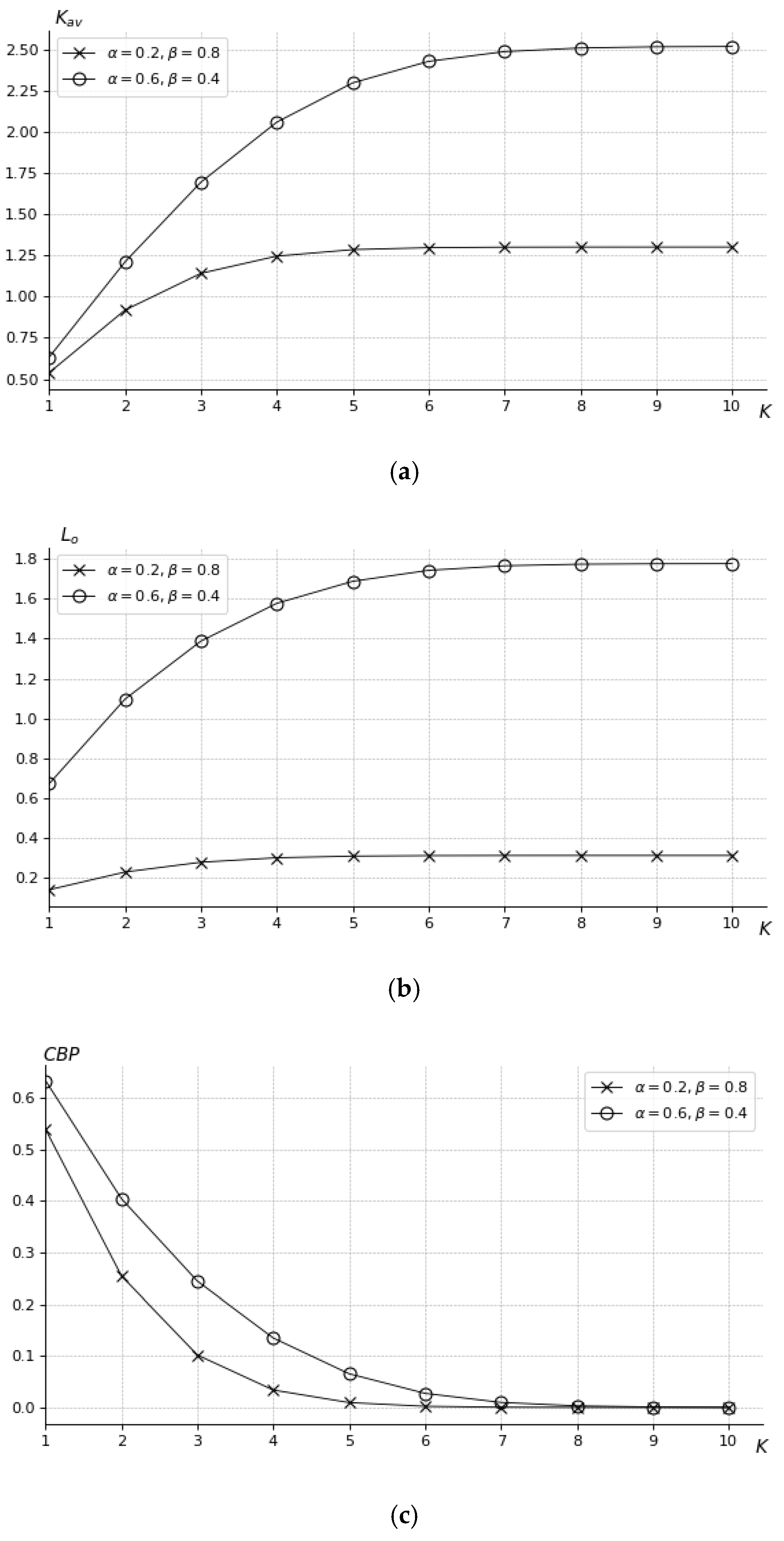
Next we considered the second goal, i.e., we studied the behavior of the performance measures of the system versus the feedback and retrial probabilities. First, we considered the systems with state-independent feedback and retrial probabilities. The corresponding results for the initial data indicated above and for $R=10$ are shown in Figure 4. It can be seen from the graphs that a simultaneous increase in the feedback probability and a decrease in the probability of loss from orbit when all channels were occupied led to an increase in all performance measures of the system. With an increase in the number of channels, the functions K_av and $L_o$ grew with high speed (see Figure 4a,b), while the values of the function $CBP$ approached each other for the selected pairs of parameters $\left(\alpha ,\beta \right)$ (see Figure 4c).

Next, we considered the behavior of the performance measures from Equations (3) and (5) for the systems with state-dependent feedback and retrial probabilities.

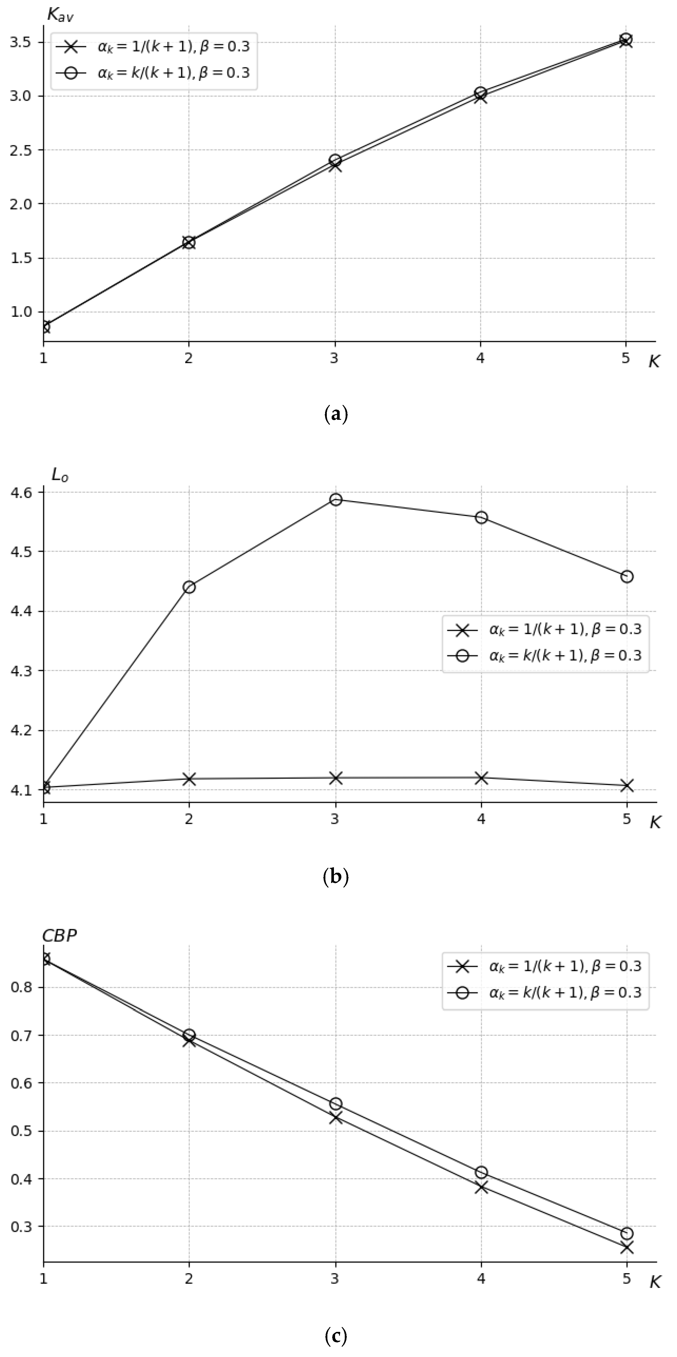
The results for the system with state-dependent feedback probabilities and constant retrial probabilities for $R=5$ are shown in Figure 5. Here we considered two schemas for the values of feedback probabilities. In the first scheme parameters ${\alpha }_k$ increased with respect to $k$, i.e., ${\alpha }_k=k/\left(k+1\right)$, while in the second one ${\alpha }_k$ decreased with respect to $k$, i.e., ${\alpha }_k=1/\left(k+1\right),k=1,\dots ,K.$ It can be seen from the graphs that in both schemas values of performance measures $K_{av}$ (see Figure 5a) and $CBP$ (see Figure 5c) were almost the same. However, values of performance measure $L_o$ (see Figure 5b) depended on the scheme of changing of feedback probabilities. For any number of channels, increasing of feedback probabilities led to an increase in the number of calls in orbit. This fact was an expected one since with the increase of the feedback probabilities, the intensity of calls into orbit increases. From Figure 5b it can be seen that in the first scheme for changing the feedback probabilities, the number of calls in the orbit took its maximum value at $K=3$, and then it decreased. This result at first glance seemed unexpected. In this regard, we noted that unlike the case of state-independent feedback probabilities (see Figure 4b) here, behavior of function $L_o$ essentially depended on the distribution of the number of busy channels. In addition, distribution of the number of busy channels in turn depended on all structural and load parameters of system. Therefore, it was impossible to predict behavior of this function in the case of state-dependent feedback probabilities.

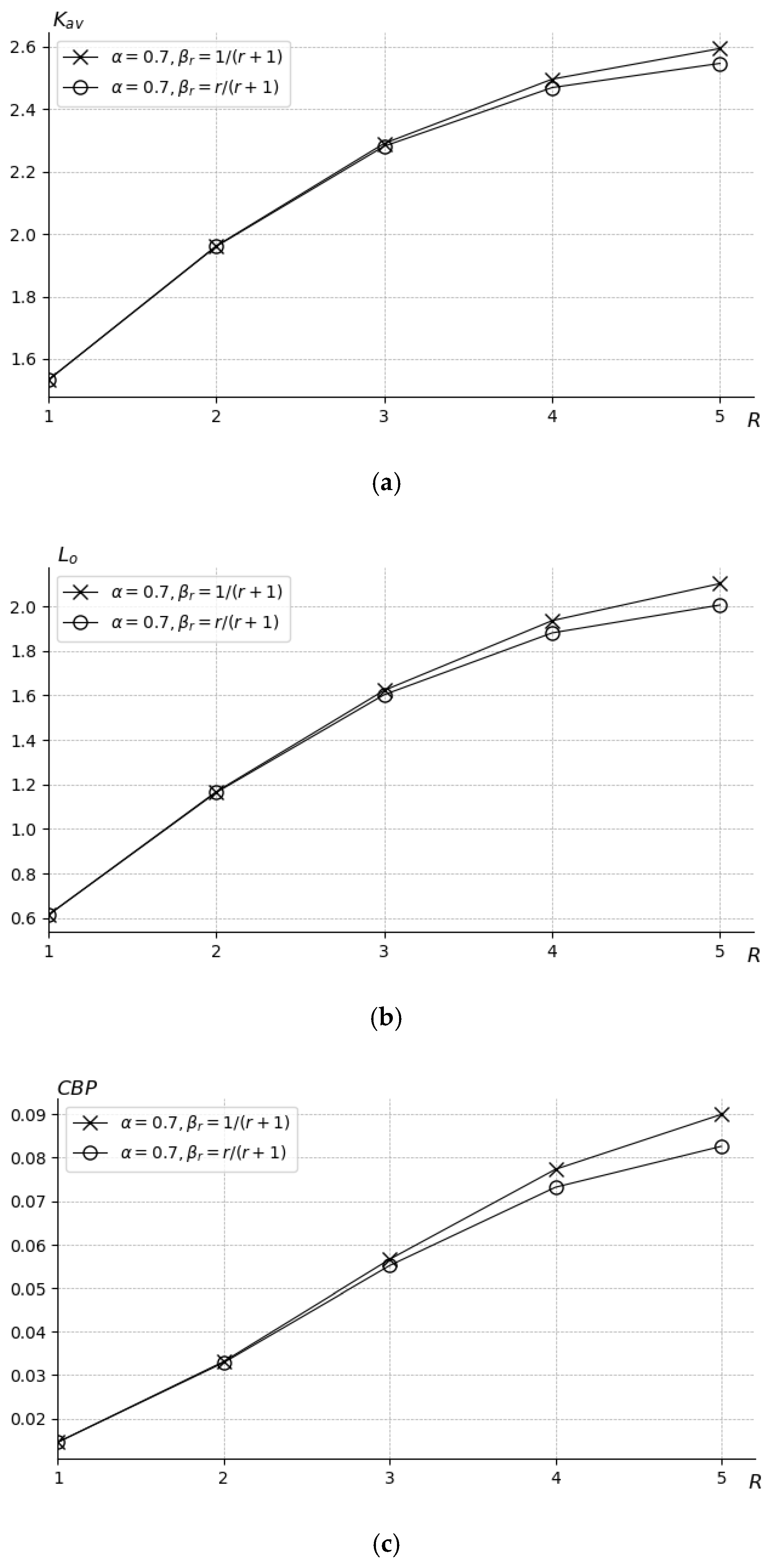
The results for the system with state-dependent retrial probabilities and constant feedback probabilities for $K=5$ are shown in Figure 6. Here we also consider two schemas for the values of retrial probabilities. In the first scheme parameters ${\beta }_r$ increased with respect to $r$, i.e., ${\beta }_r=r/\left(r+1\right)$, while in the second one ${\beta }_r$ are decreased with respect to $r$, i.e., ${\beta }_r=1/\left(r+1\right),r=1,\dots ,R.$ Unlike the previous figures here all performance measures were increasing ones and their values were almost independent of the retrial probabilities variation schemes. Note that from these graphs we concluded that for large restrictions on the orbit size, the values of all performance measures turned out to be slightly smaller in the first scheme. These facts were expected, since with an increase in the probability of leaving the system, the number of calls in orbit decreased and therefore the average number of busy channels as well as the probability that all channels were busy decreased.

6. Conclusions

The paper proposes mathematical models of multichannel systems with an MMPP flow and delayed feedback, in which the feedback is carried out by returning part of the initial calls for receiving repeated service. The probabilities of feedback or departure depend on the current number of busy channels in the system. In addition, the probabilities of reneging of calls from orbit without receiving re-service or returning to orbit for re-circulation (if all the system channels are busy upon their arrival) depend on the number of calls in orbit. We studied models with finite orbit sizes for feedback calls and developed exact and approximate methods for calculating their characteristics.

As directions for further research, the study of similar models in the presence of a Markov Arrival Process (MAP) flow of initial calls and phase-type (PH) distribution for the service time of heterogeneous calls is proposed. Of particular interest are also the problems of optimizing systems with feedback regarding the selected criteria for the quality of their functioning. These problems are the subject of special studies.

References

- Takacs, L. A Single-Server Queue with Feedback. Bell Syst. Tech. J. 1963, 42, 505–519. [Google Scholar] [CrossRef]
- Takacs, L. A Queuing Model with Feedback. Oper. Res. 1977, 11, 345–354. [Google Scholar] [CrossRef]
- Melikov, A.Z.; Ponomarenko, L.A.; Rustamov, A.M. Methods for Analysis of Queuing Models with Instantaneous and Delayed Feedbacks. Commun. Comput. Inf. Sci. 2015, 564, 185–199. [Google Scholar]
- Ayyapan, G.; Subramanian, A.M.G.; Sekar, G. M/M/1 Retrial Queuing System with Loss and Feedback under Non-pre-emptive Priority Service by Matrix Geometric Method. Appl. Math. Sci. 2010, 4, 2379–2389. [Google Scholar]
- Ayyapan, G.; Subramanian, A.M.G.; Sekar, G. M/M/1 Retrial Queuing System with Loss and Feedback under Pre-Emptive Priority Service. Int. J. Comput. Appl. 2010, 2, 27–34. [Google Scholar] [CrossRef]
- Neuts, M.F. Matrix-Geometric Solutions in Stochastic Models: An Algorithmic Approach; John Hopkins University Press: Baltimore, MA, USA, 1981; p. 332. [Google Scholar]
- Bouchentouf, A.A.; Belarbi, F. Performance Evaluation of Two Markovian Retrial Queuing Model with Balking and Feedback. Acta Univ. Sapientiae, Math. 2013, 5, 132–146. [Google Scholar] [CrossRef]
- Choi, B.D.; Kim, Y.C.; Lee, Y.W. The M/M/c Retrial Queue with Geometric Loss and Feedback. Comput. Math. Appl. 1998, 36, 41–52. [Google Scholar] [CrossRef]
- Krishna Kumar, B.; Rukmani, R.; Thangaraj, V. On Multiserver Feedback Retrial Queue with Finite Buffer. Appl. Math. Model. 2009, 33, 2062–2083. [Google Scholar] [CrossRef]
- Do, T.V. An Efficient Computation Algorithm for a Multiserver Feedback Retrial Queue with a Large Queuing Capacity. Appl. Math. Model. 2010, 34, 2272–2278. [Google Scholar] [CrossRef]
- Mitrani, I.; Chakka, R. Spectral Expansion Solution for a Class of Markov Models: Application and Comparison with the Matrix-Geometric Method. Perform. Eval. 1995, 23, 241–260. [Google Scholar] [CrossRef]
- Mokaddis, G.S.; Metwally, S.A.; Zaki, B.M. A Feedback Retrial Queuing System with Starting Failures and Single Vacation. Tamkang J. Sci. Eng. 2007, 10, 183–192. [Google Scholar]
- Fisher, W.; Meier-Hellstern, K. The Markov-Modulated Poisson Process (MMPP) Cookbook. Perform. Eval. 1992, 18, 149–171. [Google Scholar] [CrossRef]
- Melikov, A.Z.; Zadiranova, A.; Moiseev, A.N. Two Asymptotic Conditions in Queue with MMPP Arrivals and Feedback. Commun. Comput. Inf. Sci. 2016, 678, 231–240. [Google Scholar]
- Sztrik, J.; Efrosinin, D. Tool Supported Reliability Analysis of Finite-Source Retrial Queues. Autom. Remote Control 2010, 71, 1388–1393. [Google Scholar] [CrossRef]
- Berczes, T.; Sztrik, J.; Toth, A.; Nazarov, A. Performance Modeling of Finite-Source Retrial Queueing Systems with Collisions and Non-reliable Server Using MOSEL. Commun. Comput. Inf. Sci. 2017, 700, 248–258. [Google Scholar]
- Melikov, A.Z.; Ponomarenko, L.A.; Sztrik, J. Hierarchical Space Merging Algorithm for Analysis of Two Stage Queuing Network with Feedback. Commun. Comput. Inf. Sci. 2016, 638, 238–249. [Google Scholar]
Figure 1.
Structure of the queuing system MMPP/M/K/K with delayed feedback.
Figure 2.
Fragment of the transition graph for the splitting model with state space En.
Figure 3.
Graph of the splitting model with state space
Figure 4.
Dependency (a), (b) and CBP (c) on for state-independent feedback and retrial probabilities.
Figure 5.
Dependency (a), (b) and CBP (c) on for state-dependent feedback probabilities.
Figure 6.
Dependency (a), (b) and CBP (c) on for state-dependent retrial probabilities.