Sine-Cosine Algorithm to Enhance Simulated Annealing for Unrelated Parallel Machine Scheduling with Setup Times

Abstract

This paper presents a hybrid method of Simulated Annealing (SA) algorithm and Sine Cosine Algorithm (SCA) to solve unrelated parallel machine scheduling problems (UPMSPs) with sequence-dependent and machine-dependent setup times. The proposed method, called SASCA, aims to improve the SA algorithm using the SCA as a local search method. The SCA provides a good tool for the SA to avoid getting stuck in a focal point and improving the convergence to an efficient solution. SASCA algorithm is used to solve UPMSPs by minimizing makespan. To evaluate the performance of SASCA, a set of experiments were performed using 30 tests for 4 problems. Moreover, the performance of the proposed method was compared with other meta-heuristic algorithms. The comparison results showed the superiority of SASCA over other methods in terms of performance dimensions.

1. Introduction

In recent years, parallel machine scheduling problems (PMSPs) have attracted significant attention because they are used in different industrial applications and considered to be important key factors for sustainability at the operational level [1,2,3]. This kind of problems aims at assigning a set of jobs to a number of parallel machines with satisfying the requirements of the customers [4]. In general, there are three classes of the PMSPs, namely uniform, identical, and unrelated parallel machine scheduling problem (UPMSPs). However, the uniform and identical are considered as special cases of the UPMSPs, where different machines have different capabilities that are used to perform the same function. Also, if the processing times of the jobs are dependent on the machine to which these jobs are assigned, the machines are called unrelated machines.

The UPMSPs have been applied to different applications such as the mass production lines that use banks of machines with different capabilities and age to perform production tasks and those that are used in drilling operations in a printed circuit board factory [5] and scheduling jobs on a printed wiring board manufacturing line [6]. In addition, they are used in the textile industry and tested models as in [7], and the dicing of semiconductor wafer manufacturing [8]. There are several other applications, including multiprocessor computers and docking systems for ships [9].

In general, the UPMSPs are considered as a set of N jobs that must be executed on only one machine M from a set of unrelated parallel machines ($R_M$) minimizing the makespan ($C_{max}$), where the nth job consists of a single task that demands a given processing time. In addition, the sequence-dependent setup times ($S_{ijk}$) between the jobs is studied since it is a very common issue in the industry. This means that there exists a difference between the setup time required for two consecutive jobs (i and j) on machine $k,k=1,\cdots ,M$ and the reverse two jobs (i.e., the setup time on machine k between the jobs j and i). Also, the setup time between the jobs i and j on machine k is different from the setup time of the same jobs on another machine $k1$ (i.e., there exists a unique setup $N\times N$ matrix for each machine) [10]. According to these definitions, this problem can be represented as $R_M/S_{ijk}/C_{max}$.

The UPMSPs are considered as an NP-hard problem and they are extremely important requirements in practice [11]. According to this information, the traditional algorithm can be used to find the optimal solution for a small number of instances; however, if the problem has a large number of instances it is very difficult. Therefore, several methods have been proposed to solve the UPMSPs that considered the setup times [12], and they provide good results. Examples of these methods are simulated annealing (SA) [13,14], Tabu Search (TS) algorithm [15], and firefly algorithm [16].

In this paper, an alternative method is proposed to solve the UPMSPs, which is a hybrid between the SA algorithm and Sine Cosine Algorithm (SCA). The SCA is used to improve the exploitation ability of SA, where SA is used as a local search method. The proposed algorithm, namely SASCA, starts by generating a random integer solution that represents the solution for the UPMSPs. This solution has dimensions equal to the number of jobs and each value of it refers to the machine index in which the job must be performed on it. The next step of the proposed method is to select a new solution from the neighbors of the current solutions and compare the quality of them and select the best to represent the current solution. However, to ensure the ability of SA to avoid getting stuck in a local point, the operators of SCA is used to improve the current solution in which the sine and cosine functions are used. The previous steps are repeated until the stop conditions are met.

The main contributions of this paper can be summarized as:

• A newly proposed method combines the SA and SCA to update the solutions by their properties. Based on these properties the convergence toward the optimal solution increased.
• The proposed method aims at minimizing the makespan in solving the unrelated parallel machine scheduling problem (UPMSP) with sequence-dependent and machine-dependent setup times.
• A comparison is provided between the proposed method and other meta-heuristics algorithms.

The rest of this paper is organized as the following: Section 2 gives a review of some related works for the recent UPMSP methods. Section 3 presents the preliminaries about the Mixed Integer Programming for the UPMSP, Simulated Annealing Algorithm, and Sine Cosine Algorithm. In Section 4, the proposed method based on the hybrid between the SA and SCA is introduced to solve the UPMSP problem. Section 5 presents the results and discussion of the proposed method against the other algorithms. The conclusion and future works are presented in Section 6.

2. Literature Review

Several meta-heuristic algorithms have been used to solve UPMSPs in the literature [16]. For example, Logendran et al. [17] proposed a different six algorithms based on the TS to solve the same problem. In contrast, Bozorgirad and Logendran [18] used the TS algorithm to solve the sequence-dependent group-scheduling problem using unrelated-parallel machines; however, the time of execution for every job differs on different machines. Another Tabu search method based on a hybrid concept was proposed in [19] which combined the properties of the variable neighborhood descent approach with the TS algorithm. This algorithm was used to solve UPMSP with sequence-dependent setup times and unequal ready times and the objective function was the weighted number of tardy jobs.

In addition, Eva and Rubén [20] provided a method based on the improvement of the Genetic Algorithm (GA) to solve the same problem but with sequence-dependent setup times. In this modified version of GA, the fast local search and a local search enhanced crossover operator are used. Duygu et al. [21] proposed hybrid GA with a local search method that aimed at the same problem except the modification was to minimize the relocation operation of random key numbers for genes. Also, the GA was proposed in [22] to minimize the total completion time and the number of tardy for UPMSPs with sequence-dependent and machine-dependent setup times, due-times, and ready times.

The Ant Colony Optimization (ACO) algorithm was used to solve the unrelated PMSPs as in [23] which provides results better than TS algorithm and a heuristic algorithm, called Partitioning Heuristic (PH) proposed in [24]. The author of [23] proposed an extension to this study in [25]. They highlighted the difference between the two methods, whereas, in [23] the performance of ACO was evaluated over only preliminary tests where the parameters of ACO were selected by trial and error. Also, a small number of instances and limited problem structures were used, and the results of ACO was only compared with PH and TS. However, in [25], the results were compared with Metaheuristic for Randomized Priority Search (MetaRaPS) [26]. Moreover, another enhancement of ACO was introduced by the same authors to solve the same problem as in [27] which enhanced the parameters of ACO such as pheromone. The authors concluded that the result of the ACO-II was better than the ACO-I, MetaRaPS, and Simulated Annealing (SA). Lin and Hsieh [28] used a modified version of ACO algorithm to solve unrelated PMSOs with set-up times and ready times for minimizing the total weighted tardiness. They proposed a heuristic and iterated hybrid metaheuristic methods to solve the problem and according to the evaluation results, the IHM was better than the ACO and TS.

Sheremetov et al. [29] presented a two-stage GA algorithm to solve UPSMPs of the steam generators for oil cyclic steam stimulation. They considered this petroleum problem as a parallel uniform machine scheduling and they addressed the makespan and the job’s tardiness.

Nguyen and Toggenburger [2] proposed a mixed-integer linear programming scheme to address the scheduling problem of the identical machines with an additional resource. Ezugwu [30] presented a solution method to non-pre-emptive UPMS problems to minimize the makespan. Three methods were proposed to solve UPMS problems, namely SA, Hybrid Symbiotic Organisms Search with SA, and Organisms Search algorithm. As the author described, these algorithms outperform existed methods in case of 120 jobs with 12 machines. In addition, a modified differential evolution algorithm was proposed to improve the consumption of energy problem for the UPSMPs [31]. The developed method characterized each job by determining speed vectors. In [15], the TS algorithm was applied to large scale UPSMPs according to its multiple-jump strategy. Bektur and Saraç [12] developed the performance of SA and TS by combining both of them together with a mixed-integer linear programming scheme as an alternative UPSMPs method. This method aims to minimize the total weighted tardiness of the UPSMPs.

In the same context, the SA algorithm was used to solve the unrelated PMSP with machine-independent sequence-dependent setup times for which the total tardiness was the objective function used as in [32]. However, the SA suffers from some limitations, similar to other single-based meta-heuristic algorithms, such as with increasing the number of jobs, the number of solutions generated from the neighborhood extremely grows. Therefore, determining an efficient solution needs a large computation time, also there is a high probability that the SA can get stuck in a local point. Therefore, all of these points motivated us to provide an alternative method to solve the UPMSP by improving the SA algorithm using the Sine Cosine Algorithm (SCA).

The SCA is a meta-heuristic algorithm proposed in [33] to solve the global optimization problems. The solutions are updated in SCA through using either the sine or the cosine functions. The SCA has a small number of parameters and also its ability to find the optimal solution is better than other metaheuristic (MH) algorithms; therefore, the SCA has been used in many fields. For examples, Elaziz et al., in [34] applied SCA to solve features selection problem; whereas, in [35] SCA was used to select the relevant features to enhance the performance of classification the galaxy images. The authors of [36] efficiently applied SCA to train the feed-forward neural network. Moreover, the improvement of the data clustering by the SCA was used to determine the cluster centers process [37]. Ramanaiah and Reddy [38] solved the Unified Power Quality Conditioner (UPQC) problem using the SCA. Also, the SCA was applied to estimate the parameters of the kernel of Support Vector Regression (SVR) [39].

3. Preliminaries

3.1. Mixed Integer Programming Mathematical Model

The basic concepts of the Mixed Integer Programming (MIP) for the UPMSP with sequence–dependent setup times are discussed in this section. Following [24,26], the MIP formulation is given as

$$Min{C}_{max}$$

(1)

Subject to

$$\sum _{i=0,i\ne 1}^N\sum _{k=1}^M{x}_{ijk}=1;\forall j=1,\cdots ,N$$

(2)

$$\sum _{i=0,i\ne h}^N{x}_{ihk}-\sum _{j=0,j\ne h}^N{x}_{hjk}=0;$$

(3)

Equation (3) is performed $\forall h=1,\cdots ,N,k=1,\cdots ,M$.

$$C_j\ge C_i+\sum _{k=1}^M{x}_{ijk}(S_{ijk}+p_{ik})+V(\sum _{k=1}^M{x}_{ijk}-1),$$

(4)

where $i=0,\cdots ,N$

$$\sum _{j=0}^N{x}_{0jk}=1,\forall k=1,\cdots ,M$$

(5)

$$C_j\le C_{max},\forall i=1,\cdots ,N,$$

(6)

$$x_{ijk}\in 0,1,\forall i=0,\cdots ,N,\forall j=1,\cdots ,n,\forall k=1,\cdots ,M,$$

(7)

$$C_0=0$$

(8)

$$C_j\ge 0,\forall j=0,\cdots ,N$$

(9)

where $C_{max}$, $C_j$, $p_{jk}$ and $S_{ijk}$ represent maximum completion time (makespan), completion time of job j, processing time of job j on machine k, and sequence-dependent setup time to process job j after job i on machine k, respectively. Also, $x_{j0k}$: 1 if job j is the last job to be processed on machine k and 0 otherwise. The $x_{ijk}$ is 1 if job j is processed directly after job i on machine k and 0 otherwise. The $S_{0jk}$ represent Setup time to process job j first on machine k. The $x_{0jk}$ is 1 if job j is the first job to be processed on machine k and 0 otherwise. While, $N,M$ and V represent the number of jobs, the number of machines, and a large positive number, respectively.

Equation (1) represents the objective function that is used to minimize the makespan. To ensure that every job is assigned to exactly one machine and it is scheduled only once, the constraint set in Equation (2) is used. Meanwhile, the constraint (3) ensures that there exists only one preceding job and only one succeeding job. The constraint set (4) is used to compute the completion times of the jobs at the machines and to satisfy that no job can succeed and precede the same job. This can be ensured through using a large positive number (i.e., $V=\infty$) such that if job j is scheduled after job i, then ${\sum }_{k=1}^M{x}_{ijk}=1$, and therefore, $V({\sum }_{k=1}^M{x}_{ijk}-1)=0$ and $C_j=C_i+S_{ijk}+p_{jk}$. Otherwise, if job j is not scheduled right after job i, then ${\sum }_{k=1}^M{x}_{ijk}=0$, and therefore, $V({\sum }_{k=1}^M{x}_{ijk}-1)=-V$.

Set (5) is used to ensure that only one job is scheduled first at every machine. Furthermore, to ensure that $C_{max}$ is larger than the completion time of any other job, the constraint (6) is used. Also, the value of the solution x is a binary value over all the search space as stated in constraint (7). The constraints (8) and (9) state that the completion time is set to zero for the job 0, and completion times are set to non-negative values, respectively.

3.2. Simulated Annealing Algorithm

In this section, the basic concepts of the Simulated Annealing (SA) algorithm are introduced. The SA algorithm is classified as a single-based solution method which simulates the annealing process in metallurgy [40]. This process is performed through heating and cooling a metal, which increases the size of crystals and generates uniform crystals with decreasing their defects. The SA algorithm starts by generating a random solution X then it selects another solution Y from the neighborhood of X. Then the fitness function for the two solutions is computed and if the $f\left(Y\right)$ is better than $f\left(X\right)$ then the solution X is replaced by Y. Otherwise, there is a chance the solution X can be replaced by Y with a probability that decreased with increasing the difference between fitness functions of the two solutions (i.e., $▵E=f\left(X\right)-f\left(Y\right)$), this probability is defined as:

$$Prob=e^{-▵E/kT}$$

(10)

where k is the Boltzmann constant, and T is the current temperature value. If $Prob$ is greater than a random number, then $X=Y$; otherwise X not changed. After that, the SA algorithm reduces the value of the current temperature (T) using the following equation:

$$T=\beta T$$

(11)

where $\beta$ is random number chosen form the interval $[0,1]$.

3.3. Sine Cosine Algorithm

The Sine Cosine Algorithm (SCA) was proposed by Mirjalili [33] as a population-based metaheuristic algorithm in which it used the sine and cosine functions to search for the optimal solution. Therefore, the SCA algorithm, similar to other MH algorithms, starts by generating a set of N solutions called X using the following equation

$$x_i=l_i+rand\times (u_i-l_i),i=1,\cdots ,N$$

(12)

where $u_i$ and $l_i$ represent the upper and lower boundary, respectively, of the search space. The next step in the SCA is to evaluate the performance of each solution $x_i\in X$ through computing its fitness function. After that, the solution will be updated by using either sine or cosine function based on the probability random variable $r_1\in [0,1]$ as in the following equation:

$$x_i^{t+1}=\left\{\begin{array}{c}{x}_i^t+r_2\times sin\left(r_3\right)\times |r_4{x}_b^t-x_i^t|,r_1>0.5\\ x_i^t+r_2\times cos\left(r_3\right)\times |r_4{x}_b^t-x_i^t|,r_1\le 0.5\end{array}\right.$$

(13)

where $x_b$ represents the best solution, and $r_i\in [0,1],i=2,3,4$ represents a random number. The aim of the $r_2$ is to determine the optimal region for the updated solution, this region may be in the area between the current solution and the best solution or outside. Also, it is used to balance exploration and exploitation through updating its values as [33]:

$$r_2=a-t\frac{a}{t_{max}}$$

(14)

where $a,t$ and $t_{max}$ are the constant value, the current iteration and the maximum number of iteration, respectively. Also, the aim of $r_3$ is to determine if the current solution will move in the direction of the best solution $x_b$ or in direction outwards the best solution. While the aim of the $r_4$ is to give $x_b$ a random weight to stochastically asserts ($r_4>1$) or stochastically de-asserts ($r_4<1$) the effect of desalination in defining the distance.

4. Proposed Method

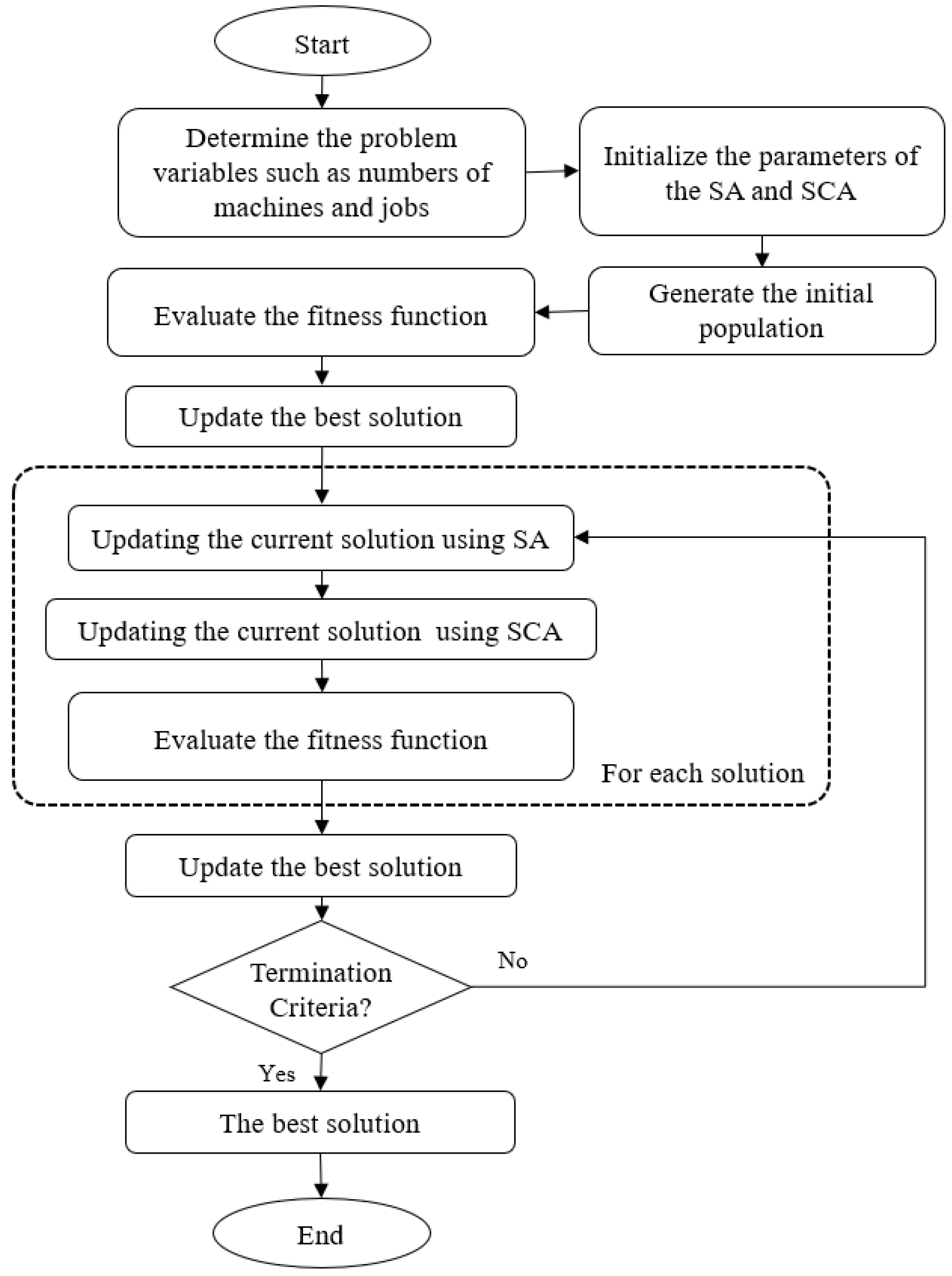
In this section, the proposed method to solve an unrelated parallel machine scheduling problem with setup times is introduced (as in Figure 1). This proposed method is called SASCA where the SCA is used to enhance the local search ability of the SA.

In general, the proposed SASCA starts by generating a random integer solution that represents the solution to UPMSPs. Then the SA generates a new solution Y from the neighboring ($N\left(X\right)$) of the current solution X. The objective function (that aimed to minimize the makespan) is computed for both solutions and if the $f\left(Y\right)<f\left(X\right)$ then $X=Y$. Otherwise, the new solution can be replaced X with probability $Pro>\alpha (\alpha \in [0,1\left]s\right)$ ($rand\in [0,1]$) that is computed based on the difference between the objective function values of both solutions (X and Y). Thereafter, the SCA is used to enhance the X through using its strategy. If the new solution is better than the old one then it will replace it, then the temperature T is decreased after performing $I_{iter}$. The previous steps are discussed with more details in the following.

4.1. Initial Solution

The proposed SASCA starts by determining the initial value for each parameter such as the current temperature $T=T0$. Then it generates a random integer solution X with dimension $N_J$ (the number of jobs) and it takes value from the interval $[1,N_m]$. For example, consider we have 15 Jobs and 3 machines, then, the representation of the solution X can be given as $[x_1,x_2,\cdots ,x_{N_J}]=\left[123231331122312\right]$. This means that the jobs 1, 6, 9, 10, 14 will be performed on machine number one, jobs 2, 4, 11, 12, 15 on machine number two, and jobs 3, 5, 7, 8, 13 on machine number three.

The next step in this stage is to compute the fitness function for the solution X using Equation (1) (that represents $C_{max}$) and select the best solutions.

4.2. Updating Solution

The updating of the solution starts by selecting solution Y from the neighbor $N\left(X\right)$ of the solution X and compute its fitness function $f\left(Y\right)$. The difference between the $f\left(X\right)$ and $f\left(Y\right)$ is computed (which represents by $▵E$). Then if $f\left(Y\right)\le f\left(X\right)$ then the solution X will be replaced by Y. Meanwhile, if this condition not satisfied, then there is another probability the solution Y can replace X (this probability is defined in Equation (10)). If $Prob>\alpha$ then $X=Y$. Thereafter, the next step is to use the operators of SCA algorithm to improve the exploitation ability of SA algorithm as the following: first, the value of the parameter $r_2$ is updated using Equation (14) also, the value of parameters $r_1,r_3$ and $r_4$ are updated. Then based on the value of $r_1$ the current solution X will be updated using either the sine or cosine function as in Equation (13). The next step is to update the best solution $X_b$ and reduce the temperature as in Equation (11), after running the inner $I_{iter}$ from the previous decreasing value of T. The algorithm is stopped if the terminal criteria are met.

The entire steps of the proposed method are illustrated in Algorithm 1.

Algorithm 1 The steps of the proposed method

1: Input: $T_0$ initial temprature, Size of population N, dimension of solution $N_J$, and total number of generations $t_{max}$. 2: Output: The best solution $x_b$. 3: Set the initial value of N solutions with dimension $N_J$. 4: Evaluate the quality of each $X_i$ by computing its fitness value $F_i$, and update number of fitness evaluation. 5: Find the best solution $X_b$. 6: Put $t=1$. 7: repeat 8:  for $i=1:N$ do 9:   $X_i^{New}=$ determine the neighbor solution of $X_i$. 10:   Compute the fitness value $f\left(X_i^{New}\right)$ for $X_i^{New}$. 11:   if $f\left(X_i^{New}\right)<f\left(X_i\right)$ then 12:    $X_i=X_i^{New}$. 13:   else 14:    $\delta =f\left(X_i\right)-f\left(X_i^{New}\right)$. 15:    if ($exp(-\delta /T)\le r_5$) then 16:     $X_i=X_i^{New}$. 17:    end if 18:   end if 19:   Update the temprature T using Equation (11). 20:  end for 21:  for $i=1:N$ do 22:   Update the parameters $r_1,r_2,r_3$, and $r_4$. 23:   Update $X_i$ using Equation (13). 24:   Evaluate the quality of each $X_i$ by computing its fitness value $F_i$. 25:  end for 26:  Find the best solution $X_b$. 27:  Set $t=t+1$. 28: until$t<t_{max}$

5. Experiments and Results

In this section, the dataset description, experiment settings, and the discussion of the results are presented. The experiments are divided into two parts, the first one contains the results of the proposed algorithm and the other metaheuristic algorithms such as grey wolf optimization, particle swarm optimization, genetic algorithm in addition to the traditional SA. The second one compare the results of the proposed SASCA with other state-of-the-art methods. Then, the results of the average percent deviations are provided followed by the influence of the ($\beta$) variable on the proposed SASCA.

5.1. Dataset Description

We conducted 30 tests for 4 problems, each problem has its machines and jobs. The first problem has 2 machines with 11 kinds of jobs (i.e., 6, 7, 8, 9, 10, 11, 40, 60, 80, 100, and 120 jobs). The second problem has 4 machines with 10 kinds of jobs (i.e., 6, 7, 8, 9, 10, 11, 60, 80, 100, and 120 jobs). The third problem has 6 machines with 8, 9, 10, 11, 100 and 120 jobs, whereas, the last problem has 8 machines with 10, 11, and 120 jobs. These jobs were selected as in [24,25] to evaluate the proposed method on small and large jobs. In this manner, Equation (15) is applied to select large jobs. For instance, 100/8 = 12.5; so, job 100 is ignored from machine 8 and 120 is selected.

$$SelectJobif(Jobs/Machine)>15$$

(15)

For more information about the dataset used in this paper is available at [41].

5.2. Experiment Settings

The experiments were performed on “Windows 10” with CPU “Core2Due” and 4GB RAM. Each job, in all problems, was evaluated over 15 different problem instances and the average value of $C_{max}$ is calculated. The proposed method used a stop condition equals to 25 for the small problems and 10000 iterations for the large problems to record the best obtained value of fitness function ($C_{max}$). For a fair comparison, the number of iterations is chosen to meet the same setting in the references. The parameters setting of the proposed method are listed in

Table 1. The parameters setting of the proposed method.

Algorithm	Parameters Setting
SASCA	$Initialtemperature\left(T0\right)$ = 10,
	$temperaturereductionrate\left(\beta \right)$ = 0.97, $parameter\left(a\right)$ = 2,
	$parameter\left(r1\right)\in [2,0]$
SA	$Initialtemperature=10$, $temperaturereductionrate=0.97$,
	$localstep$ = 1
GWO	$Parameter\left(a\right)\in [2,0]$
PSO	$Inertiaweight\left(w\right)=1,inertiaweightdampingratio\left(wDamp\right)=0.99$,
	$personallearningcoefficient\left(c1\right)=1,globallearningcoefficient\left(c2\right)=2$
GA	$Crossoverprobability\left(pc\right)=0.8,extrarangefactorforcrossover\left(\gamma \right)=0.2$,
	$mutationpercentage\left(pm\right)=0.3,mutationprobability\left(mu\right)=0.02,selectionpressure\left(sp\right)=8$

. In general, these parameters are selected based on the experiments besides, they showed good performances in our previous works such as [42,43,44,45].

5.3. Comparison with Metaheuristic Methods

In this experiments, the performance of the SASCA is compared with other four MH methods as given in

Table 2. Average of $C_{max}$ values of the small problems for each algorithm (best results are in boldface).

M	J	SASCA	SA	GWO	PSO	GA
2	6	357.33	362.60	378.33	372.56	375.38
2	7	453.00	470.20	504.80	505.80	572.67
2	8	512.00	513.67	530.88	531.25	530.88
2	9	566.67	624.47	598.33	592.20	617.25
2	10	639.33	692.20	681.67	677.56	664.86
2	11	716.00	788.40	744.50	752.25	743.75
4	6	224.67	247.27	276.80	280.30	276.80
4	7	212.33	266.60	256.00	292.17	291.00
4	8	251.00	327.13	344.40	344.40	333.00
4	9	342.00	376.73	364.00	367.33	360.00
4	10	340.33	398.47	358.00	367.75	367.75
4	11	368.33	434.80	413.00	442.00	450.00
6	8	214.67	244.67	221.25	223.00	219.33
6	9	242.33	267.60	242.90	307.50	334.00
6	10	228.67	295.20	312.00	332.00	344.67
6	11	258.00	319.67	337.00	341.00	345.00
8	10	221.67	252.00	231.33	228.67	227.00
8	11	221.33	327.67	288.00	296.00	323.00

and

Table 3. Average of the computational time of the small problems for each algorithm (best results are in boldface).

M	J	SASCA	SA	GWO	PSO	GA
2	6	0.0490	0.0545	0.0377	0.0337	0.0457
2	7	0.0541	0.0387	0.0560	0.0554	0.0597
2	8	0.0582	0.0378	0.0583	0.0584	0.0645
2	9	0.0586	0.0474	0.0594	0.0591	0.0768
2	10	0.0629	0.0445	0.0647	0.0600	0.0794
2	11	0.0590	0.0330	0.0732	0.0708	0.0914
4	6	0.0581	0.0287	0.0515	0.0468	0.0665
4	7	0.0601	0.0237	0.0592	0.0570	0.0834
4	8	0.0585	0.0295	0.0637	0.0616	0.0813
4	9	0.0613	0.0300	0.0718	0.0666	0.0883
4	10	0.0637	0.0308	0.0857	0.0805	0.1075
4	11	0.0646	0.0299	0.0892	0.0854	0.1066
6	8	0.0620	0.0283	0.0803	0.0740	0.1021
6	9	0.0652	0.0287	0.0834	0.0817	0.1052
6	10	0.0653	0.0322	0.0991	0.0899	0.1121
6	11	0.0822	0.0312	0.1134	0.1018	0.1314
8	10	0.0702	0.0412	0.1138	0.1045	0.1318
8	11	0.0723	0.0668	0.1189	0.1102	0.1324

. This comparison are performed using a set of different Jobs (i.e., 6, 7, 8, 9, 10, 11) and number of machines (2, 4, 6, 8). According to the results of the average of $C_{max}$, it can be noticed that the proposed SASCA has high ability to find the smallest $C_{max}$ among all the tested number of machines and jobs. Meanwhile, the SA has better $C_{max}$ at the small number of jobs especially at jobs 6, 7, and 8. However, when the number of machines become 6 and number of jobs become 8, the GWO gives better results than SA. By comparing, the performance of the four MH methods (i.e., GWO, PSO, SA, and GA) at 8 machines as well as 10 and 11 jobs, it can be seen that the GA and GWO provided smaller results, respectively, than the other two methods (i.e., SA, and PSO).

Moreover, by analysing the results of computational time(s), it can be observed that the SA is the fast algorithm over all the tested problems except for the case when the number of machines is 2 and jobs 6, when the PSO has the smaller CPU time(s). In addition, it can be noticed that the SASCA requires smaller CPU time(s) than the other methods.

5.4. Comparison with the State-of-the-Art Methods

In this section, we compare the performance of the SASCA and the other methods, for example, Tabu (T9) and Tabu (T8) [24] and Ant Colony Optimization (ACO) [25], Partitioning Heuristic (PH) [25], Tabu Search (TS) [24], and MRPS (Meta-RaPS) [26]. These experiments are performed through two datasets (i.e, small and large) as given in the following subsections.

5.4.1. Small Problems

Table 4. Average of $C_{max}$ values of the small problems for each algorithm (best results are in boldface).

		SASCA		SA		Tabu (T9) [24]		Tabu (T8) [24]
M	Jobs	${\mathit{C}}_{\mathit{max}}$	Time	${\mathit{C}}_{\mathit{max}}$	Time	${\mathit{C}}_{\mathit{max}}$	Time	${\mathit{C}}_{\mathit{max}}$	Time
2	6	357.33	0.0490	362.60	0.05450	397.20	0.440	395.27	0.150
	7	453.00	0.0541	470.20	0.03869	502.00	0.210	494.73	0.200
	8	512.00	0.0582	513.67	0.03778	522.07	0.260	521.20	0.080
	9	566.67	0.0586	624.47	0.04742	614.53	0.310	607.33	0.290
	10	639.33	0.0629	692.20	0.04455	649.60	0.370	645.33	0.340
	11	716.00	0.0590	788.40	0.03299	724.47	0.440	722.53	0.440
4	6	224.67	0.0581	247.27	0.02869	249.07	0.010	251.27	0.020
	7	212.33	0.0601	266.60	0.02369	259.53	0.024	264.27	0.260
	8	251.00	0.0585	327.13	0.02947	268.93	0.070	270.47	0.034
	9	342.00	0.0613	376.73	0.03004	347.73	0.930	346.47	0.860
	10	340.33	0.0637	398.47	0.03082	363.27	0.950	360.33	0.980
	11	368.33	0.0646	434.80	0.02994	375.80	0.960	376.30	0.990
6	8	214.67	0.0620	244.67	0.02832	235.47	0.034	240.27	0.290
	9	242.33	0.0652	267.60	0.02866	244.33	0.060	249.27	0.050
	10	228.67	0.0653	295.20	0.03221	254.67	0.060	259.13	0.080
	11	258.00	0.0822	319.67	0.03118	265.87	0.040	273.80	0.040
8	10	221.67	0.0702	252.00	0.04123	230.07	0.090	232.00	0.080
	11	221.33	0.0723	327.67	0.06682	232.87	0.110	235.20	0.120

illustrates the results of the SASCA and other methods. The values of the $C_{max}$ and computation time are listed in this table. The SASCA is compared with SA, Tabu(T9), and Tabu(T8). The results of the Tabu (T9) and Tabu (T8) are obtained from [24] because it used the same problems (i.e., the same numbers of machines and jobs).

From this table, we can see that the proposed method (SASCA) outperforms the other methods in all problems in terms of $C_{max}$ value followed by Tabu (T9), Tabu (T8), and SA. In terms of computation time, the proposed method ranked second after SA followed by Tabu (T8) and Tabu (T9). The SASCA was close to SA but outperformed SA in computational time, as expected, since the SCA algorithm, in general, consumes more time than SA.

5.4.2. Statistical Test for the Small Problems

The performance of the SASCA is evaluated using Wilcoxon’s rank sum test to check if there is a significant difference between the SASCA and the other methods or not in the small problems [46,47,48]. In addition, the Friedman test is applied to rank these methods. The results are given in

Table 5. Results of Wilcoxon test for the small problems (best results are in boldface).

Measure	SA	Tabu (T9)	Tabu (T8)
$C_{max}$	0.013	0.060	0.047
Time	0.000	0.041	0.006

and

Table 6. Results of Friedman test for the small problems (best results are in boldface).

	SASCA	SA	Tabu (T9)	Tabu (T8)
$C_{max}$	1	3.56	2.67	2.78
Time:	2.5	2.06	2.72	2.72

, it can be seen from the Wilcoxon test that p-value is less than 0.05 and this indicates there is a significant difference between the proposed method and other methods except Tabu (T9) in terms of $C_{max}$. In contrast, Table 6 shows that the SASCA has the smallest average rank in terms of $C_{max}$, and it achieved the second rank in CPU time(s). Therefore, it can be concluded that the proposed method can outperform the other methods in the case of small datasets.

5.4.3. Large Problems

Table 7. Average of $C_{max}$ values of the large problems for each algorithm.

M	Jobs	SASCA		ACO [25]		MRPS [26]		TS [24]		PH [25]		LB
		${\mathit{C}}_{\mathit{max}}$	$\mathit{STD}$	${\mathit{C}}_{\mathit{max}}$	$\mathit{STD}$	${\mathit{C}}_{\mathit{max}}$	$\mathit{STD}$	${\mathit{C}}_{\mathit{max}}$	$\mathit{STD}$	${\mathit{C}}_{\mathit{max}}$	$\mathit{STD}$	${\mathit{C}}_{\mathit{max}}$	$\mathit{STD}$
2	40	2398.40	39.45	2404.33	36.88	2422	35.44	2486.53	39.54	2521.47	57.28	2344.7	36.31
	60	3574.70	22.15	3575.2	33.41	3617.93	35.61	3736.47	55.61	3733.33	50.17	3510.17	36.03
	80	4737.00	11.19	4741.8	60.28	4803.27	57.62	4942.27	70.36	4926.93	74.11	4664.83	58.43
	100	5986.73	81.02	5897.6	60.68	5988.6	58.05	6180.87	73.49	6128.07	63.96	5819.23	59.80
	120	7234.87	56.93	7082.6	64.64	7196.47	71.98	7447.6	80.89	7336.53	73.79	7008.03	69.27
4	60	1715.27	28.06	1736.6	21.5	1752.4	17.71	1785.53	25.19	1817.87	26.79	1650.73	15.79
	80	2294.53	22.33	2307.8	18.68	2334.07	15.57	2370.13	22.26	2396.67	25.97	2201.48	15.94
	100	2855.00	15.42	2849.47	31.88	2867.27	20.53	2934.13	35.24	2959.93	46.61	2740.7	20.46
	120	3432.50	16.36	3404.53	25.66	3432.93	17.45	3515.13	33.15	3537.8	36.92	3291.2	16.71
6	100	1890.57	9.57	1891.07	11.38	1892.67	6.68	1940.6	14.98	1973.47	21.21	1783.03	6.12
	120	2295.80	17.33	2249.2	15.69	2252.6	14.58	2313.07	25.93	2353.67	38.37	2137.6	11.17
8	120	1684.14	7.10	1685.4	13.77	1706.8	8.93	1739.73	15.01	1778.13	48.31	1580.23	7.43

displays the results of the proposed method for large problems versus other methods. The calculated values of the $C_{max}$ and standard deviation ($STD$) for the SASCA are listed in this table along with the compared results which obtained from the state-of-the-art methods namely Ant Colony Optimization (ACO) [25], Partitioning Heuristic (PH) [25], Tabu Search (TS) [24], and MRPS (Meta-RaPS) [26]. In addition, the lower bound (LB) is listed in the last column as a reference value.

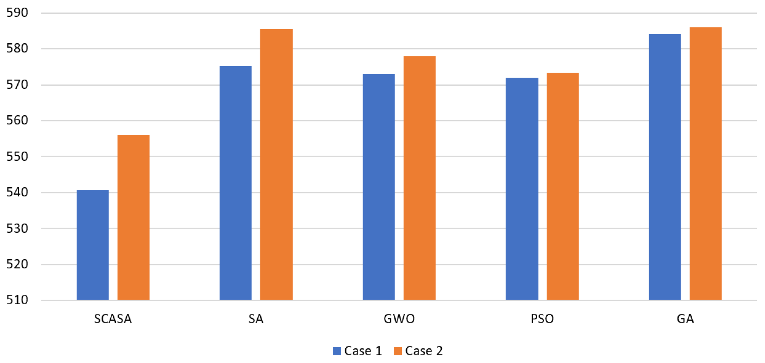
From this table, we can conclude that, in terms of $C_{max}$, the proposed method outperformed the other methods in 7 out of 12 problems and its results are closer to the reference values. Whereas, in terms of $STD$, the proposed algorithm performed better in 6 out of 12 problems followed by MRPS and ACO, respectively. These results are illustrated in Figure 2 to show the variation of $C_{max}$ among these algorithms; the values in this figure are normalized by the following equation:

$$Normalizedvalue=\frac{C_{ma{x}_{method}}-C_{ma{x}_{refrencevalue}}}{C_{ma{x}_{refrencevalue}}}$$

(16)

5.4.4. Statistical Test for the Large Problems

In this section, the two statistical tests (i.e., Wilcoxon’s rank sum and Friedman test) are used to further analyze the results of the proposed SASCA based on large problems.

Table 8. Results of Wilcoxon test for the large problems (best results are in boldface).

	ACO	MRPS	TS	PH
$C_{max}$	0.924	0.689	0.420	0.420
Time	0.140	0.687	0.021	0.001

depicts that there is no significant difference between SASCA and the other methods in terms of $C_{max}$. Meanwhile, there are significant differences between SASCA and TS and PH methods in terms of CPU time(s). The same observation is noticed from

Table 9. Results of Friedman test for the large problems (best results are in boldface).

	SASCA	ACO	MRPS	TS	PH
$C_{max}$	1.58	1.58	2.83	4.33	4.67
Time	2.33	2.42	1.67	4.00	4.58

, where the SASCA and ACO have the same average rank, followed by MRPS, TS, and PH, respectively, in terms of $C_{max}$. Moreover, in terms of the CPU time(s), the MRPS allocates the first rank followed by the SASCA which allocates the second rank, while the ACO in the third rank followed by the TS and PH, respectively.

5.5. Average Percent Deviations

The average percent deviations values ($apd$) for the small and the large problems are provided in

Table 10. The $apd$ values for the small problems for the hybrid method of Simulated Annealing algorithm and Sine Cosine Algorithm (SASCA) and the other methods.

M	Jobs	SA	Tabu(T9)	Tabu(T8)
2	6	0.015	0.112	0.106
	7	0.038	0.108	0.092
	8	0.003	0.020	0.018
	9	0.102	0.084	0.072
	10	0.083	0.016	0.009
	11	0.101	0.012	0.009
4	6	0.101	0.109	0.118
	7	0.256	0.222	0.245
	8	0.303	0.071	0.078
	9	0.102	0.017	0.013
	10	0.171	0.067	0.059
	11	0.180	0.020	0.022
6	8	0.140	0.097	0.119
	9	0.104	0.008	0.029
	10	0.291	0.114	0.133
	11	0.239	0.031	0.061
8	10	0.137	0.038	0.047
	11	0.480	0.052	0.063

and

Table 11. The $apd$ values for the large problems among SASCA and the other methods.

M	Jobs	ACO	MRPS	TS	PH
2	40	0.002	0.010	0.037	0.051
	60	0.000	0.012	0.045	0.044
	80	0.001	0.014	0.043	0.040
	100	−0.015	0.000	0.032	0.024
	120	−0.021	−0.005	0.029	0.014
4	60	0.012	0.022	0.041	0.060
	80	0.006	0.017	0.033	0.045
	100	−0.002	0.004	0.028	0.037
	120	−0.008	0.000	0.024	0.031
6	100	0.000	0.001	0.026	0.044
	120	−0.020	−0.019	0.008	0.025
8	120	0.001	0.013	0.033	0.056

to prove the superiority of the proposed method against the other methods. The $apd$ of ($C_{ma{x}_{method}}$) of each method are recorded where $apd$ is calculated as follows:

$$apd=\frac{C_{ma{x}_{method}}-C_{ma{x}_{SASCA}}}{C_{ma{x}_{SASCA}}}$$

(17)

Table 10 shows that the SASCA outperformed all algorithms in all machines and jobs. Table 11 illustrates that the SASCA outperformed the PH and TS in all large problems and got over MRPS in 10 out of 12 problems; while the SASCA works better than ACO in 7 out of 12 problems. In general, the SASCA shows good ability to work with both small and large problems.

5.6. Parameters Sensitivity

5.6.1. Influence of ($\beta$) value on the SASCA

In this subsection, the influence of ($\beta$) variable on the performance of the SASCA is evaluated. In this test, two machines are used with five types of jobs (i.e., 40, 60, 80, 100, and 120).

Table 12. Influence of the $\beta$ on the performance of the SASCA.

Job	$\mathit{\beta }=\mathbf{0.95}$		$\mathit{\beta }=\mathbf{0.5}$		$\mathit{\beta }=\mathbf{0.1}$
	${\mathit{C}}_{\mathit{max}}$	STD	${\mathit{C}}_{\mathit{max}}$	STD	${\mathit{C}}_{\mathit{max}}$	STD
40	2398.40	39.45	2416.15	31.46	2401.17	30.14
60	3574.70	22.15	3598.00	19.75	3616.00	30.61
80	4737.00	11.19	4857.13	19.71	4823.00	27.00
100	5986.73	81.02	6054.25	75.78	6083.50	74.72
120	7234.87	56.93	7337.50	49.50	7350.60	54.76

shows the $C_{max}$ and the STD values. It can be observed that the best value for the $\beta$ is 0.95 which has the smallest $C_{max}$ value followed by $\beta =0.5$. Meanwhile, in the case of $\beta =0.5$ the proposed SASCA becomes more stable than other two values. In addition, the $\beta =0.95$ is more stable than $\beta =0.1$.

5.6.2. Influence of the Parameters Setting in the Algorithms

In this section, we study the influence of the parameters setting on the performance of the MH. The values of the parameters for each algorithm are given in

Table 13. New parameters setting for testing the sensitivity of the parameters.

Algorithm	Parameters Setting
SASCA	$T0=5,\beta =0.97,a=3,r1\in [3,0]$
SA	$T0=5,\beta =0.97,localstep=1$
GWO	$a\in [3,0]$
PSO	$w=0.9,wDamp=0.2,c1=2,c2=2$
GA	$pc=0.6,mu=0.05,\gamma =0.4,pm=0.5,sp=5$

, with the same number of population and the number of iterations used in the previous experiments. Moreover, the number of machines is two and the number of jobs varies from 6 to 11. The comparison results are given in

Table 14. Average of $C_{max}$ of the small problems on 2 machines for testing the sensitivity of the parameters (best results are in boldface).

J	SASCA	SA	GWO	PSO	GA
6	372.33	391.12	390.25	388.75	389.00
7	457.50	488.11	496.60	479.40	519.67
8	512.80	536.36	535.80	534.33	539.25
9	568.00	623.50	605.75	605.00	629.60
10	696.50	700.02	689.40	681.00	688.40
11	729.67	775.45	749.75	751.50	749.75

and Figure 3. From Table 14 it can be noticed that the SASCA has the smallest $C_{max}$ overall the tested problems except at the number of jobs is 10, the PSO is the best algorithm. Whereas, Figure 3 depicts the comparison between the average of the $C_{max}$ of the parameter setting in Table 1 and the current one (i.e., Table 13). It can be noticed that the performance of the MH methods based on the value in Table 1 is better than their performance based on Table 13.

From the previous analysis, it can be observed the high performance of the SASCA method, however, there are some limitations. For example, the time computational of the SASCA needs more improvements since it updates the solutions using SA operators followed by the operators of SCA. Besides, the diversity of the solution needs to be enhanced and this can be achieved using the Disruptor operators.

6. Conclusions

Recently, unrelated parallel machine scheduling problems (UPMSPs) have received more attention due to their wide applications in various domains. To solve UPMSPs, Simulated Annealing (SA) algorithm provides suitable results compared to other meta-heuristic methods (MH) methods, but its performance still requires more improvement. Therefore, in this paper, an alternative method was proposed for determining the optimal solution to solve UPMSPs by minimizing the makespan value. The proposed method called SASCA combined the SA algorithm with Sine-Cosine Algorithm (SCA). SASCA worked in sequence order; in the first stage, the optimization process started by using SA to evaluate the problem solution, then the output solution was fed to SCA to continue the optimization process. The final solution was evaluated by the objected function. The performance of the proposed method was compared with several methods including ACO, MRPS, TS, and PH in terms of makespan values and standard deviation. In general, SASCA has the ability to solve small and large problems of unrelated parallel machine scheduling. In the future, the proposed method will be evaluated in different kinds of problems such as image segmentation, task scheduling in cloud computing, and other optimization problems.

References

1. Shim, S.O.; Park, K. Technology for production scheduling of jobs for open innovation and sustainability with fixed processing property on parallel machines. Sustainability 2016, 8, 904. [Google Scholar] [CrossRef]
2. Nguyen, N.Q.; Yalaoui, F.; Amodeo, L.; Chehade, H.; Toggenburger, P. Total completion time minimization for machine scheduling problem under time windows constraints with jobs’ linear processing rate function. Comput. Oper. Res. 2018, 90, 110–124. [Google Scholar] [CrossRef]
3. Gafarov, E.; Werner, F. Two-Machine Job-Shop Scheduling with Equal Processing Times on Each Machine. Mathematics 2019, 7, 301. [Google Scholar] [CrossRef]
4. Expósito-Izquierdo, C.; Angel-Bello, F.; Melián-Batista, B.; Alvarez, A.; Báez, S. A metaheuristic algorithm and simulation to study the effect of learning or tiredness on sequence-dependent setup times in a parallel machine scheduling problem. Expert Syst. Appl. 2019, 117, 62–74. [Google Scholar] [CrossRef]
5. Hsieh, J.C.; Chang, P.C.; Hsu, L.C. Scheduling of Drilling Operations in Printed Circuit Board Factory. Comput. Ind. Eng. 2003, 44, 461–473. [Google Scholar] [CrossRef]
6. Bilyk, A.; Mönch, L. A Variable Neighborhood Search Approach for Planning and Scheduling of Jobs on Unrelated Parallel Machines. J. Intell. Manuf. 2012, 23, 1621–1635. [Google Scholar] [CrossRef]
7. Silva, C.; Magalhaes, J.M. Heuristic Lot Size Scheduling on Unrelated Parallel Machines with Applications in the Textile Industry. Comput. Ind. Eng. 2006, 50, 76–89. [Google Scholar] [CrossRef]
8. Kim, D.W.; Na, D.G.; Chen, F.F. Unrelated Parallel Machine Scheduling with Setup times and a Total Weighted Tardiness Objective. Robot. Comput.-Integr. Manuf. 2003, 19, 179–181. [Google Scholar] [CrossRef]
9. Fanjul-Peyro, L.; Ruiz, R. Iterated greedy local search methods for unrelated parallel machine scheduling. Eur. J. Oper. Res. 2010, 207, 55–69. [Google Scholar] [CrossRef]
10. Pinedo, M.L. Scheduling: Theory, Algorithms, and Systems; Springer: Berlin, Germany, 2016. [Google Scholar]
11. Yalaoui, F.; Chu, C. An Efficient Heuristic Approach for Parallel Machine Scheduling with Job Splitting and Sequence-dependent Setup Times. IIE Trans. 2003, 35, 183–190. [Google Scholar] [CrossRef]
12. Bektur, G.; Saraç, T. A mathematical model and heuristic algorithms for an unrelated parallel machine scheduling problem with sequence-dependent setup times, machine eligibility restrictions and a common server. Comput. Oper. Res. 2019, 103, 46–63. [Google Scholar] [CrossRef]
13. Hamzadayi, A.; Yildiz, G. Event driven strategy based complete rescheduling approaches for dynamic m identical parallel machines scheduling problem with a common server. Comput. Ind. Eng. 2016, 91, 66–84. [Google Scholar] [CrossRef]
14. Hamzadayi, A.; Yildiz, G. Hybrid strategy based complete rescheduling approaches for dynamic m identical parallel machines scheduling problem with a common server. Simul. Model. Pract. Theory 2016, 63, 104–132. [Google Scholar] [CrossRef]
15. Wang, H.; Alidaee, B. Effective heuristic for large-scale unrelated parallel machines scheduling problems. Omega 2019, 83, 261–274. [Google Scholar] [CrossRef]
16. Ezugwu, A.E.; Akutsah, F. An Improved Firefly Algorithm for the Unrelated Parallel Machines Scheduling Problem With Sequence-Dependent Setup Times. IEEE Access 2018, 6, 54459–54478. [Google Scholar] [CrossRef]
17. Logendran, R.; McDonellb, B.; Smuckera, B. Scheduling unrelated parallel machines with sequence-dependent setups. Comput. Oper. Res. 2007, 34, 3420–3438. [Google Scholar] [CrossRef]
18. Bozorgirad, M.A.; Logendran, R. Sequence-dependent group scheduling problem on unrelated-parallel machines. Expert Syst. Appl. 2012, 39, 9021–9030. [Google Scholar] [CrossRef]
19. Chen, C.L. Iterated hybrid metaheuristic algorithms for unrelated parallel machines problem with unequal ready times and sequence-dependent setup times. Int. J. Adv. Manuf. Technol. 2012, 60, 693–705. [Google Scholar] [CrossRef]
20. Eva, V.; Rubén, R. A genetic algorithm for the unrelated parallel machine scheduling problem with sequence dependent setup times. Eur. J. Oper. Res. 2011, 211, 612–622. [Google Scholar]
21. Duygu, Y.E.; Ozmutlu, H.C.; Seda, O. Genetic algorithm with local search for the unrelated parallel machine scheduling problem with sequence-dependent set-up times. Int. J. Prod. Res. 2014, 52, 5841–5856. [Google Scholar]
22. Tavakkoli-Moghaddam, R.; Taheri, F.; Bazzazi, M.; Izadi, M.; Sassani, F. Design of a genetic algorithm for bi-objective unrelated parallel machines scheduling with sequence-dependent setup times and precedence constraints. Comput. Oper. Res. 2009, 36, 3224–3230. [Google Scholar] [CrossRef]
23. Arnaout, J.P.; Musa, R.; Rabadi, G. Ant colony optimization algorithm to parallel machine scheduling problem with setups. In Proceedings of the 2008 IEEE International Conference on Automation Science and Engineering, Arlington, VA, USA, 23–26 August 2008; pp. 578–582. [Google Scholar]
24. Helal, M.; Rabadi, G.; Al-Salem, A. A tabu search algorithm to minimize the makespan for the unrelated parallel machines scheduling problem with setup times. Int. J. Oper. Res. 2006, 3, 182–192. [Google Scholar]
25. Arnaout, J.P.; Rabadi, G.; Musa, R. A two-stage ant colony optimization algorithm to minimize the makespan on unrelated parallel machines with sequence-dependent setup times. J. Intell. Manuf. 2010, 21, 693–701. [Google Scholar] [CrossRef]
26. Rabadi, G.; Moraga, R.J.; Al-Salem, A. Heuristics for the unrelated parallel machine scheduling problem with setup times. J. Intell. Manuf. 2006, 17, 85–97. [Google Scholar] [CrossRef]
27. Arnaout, J.P.; Musa, R.; Rabadi, G. A two-stage ant colony optimization algorithm to minimize the makespan on unrelated parallel machines—-Part II: enhancements and experimentations. J. Intell. Manuf. 2014, 25, 43–53. [Google Scholar] [CrossRef]
28. Lin, Y.K.; Hsieh, F.U. Unrelated Parallel Machine Scheduling with Setup times and Ready times. Int. J. Prod. Res. 2014, 52, 1200–1214. [Google Scholar] [CrossRef]
29. Sheremetov, L.; Martínez-Muñoz, J.; Chi-Chim, M. Two-stage genetic algorithm for parallel machines scheduling problem: Cyclic steam stimulation of high viscosity oil reservoirs. Appl. Soft Comput. 2018, 64, 317–330. [Google Scholar] [CrossRef]
30. Ezugwu, A.E. Enhanced symbiotic organisms search algorithm for unrelated parallel machines manufacturing scheduling with setup times. Knowl.-Based Syst. 2019, 172, 15–32. [Google Scholar] [CrossRef]
31. Wu, X.; Che, A. A memetic differential evolution algorithm for energy-efficient parallel machine scheduling. Omega 2019, 82, 155–165. [Google Scholar] [CrossRef]
32. Kim, D.W.; Kim, K.H.; Jang, W.; Chen, F.F. Unrelated parallel machine scheduling with setup times using simulated annealing. Robot. Comput. Integr. Manuf. 2002, 18, 223–231. [Google Scholar] [CrossRef]
33. Mirjalili, S. SCA: a sine cosine algorithm for solving optimization problems. Knowl.-Based Syst. 2016, 96, 120–133. [Google Scholar] [CrossRef]
34. Elaziz, M.E.A.; Ewees, A.A.; Oliva, D.; Duan, P.; Xiong, S. A Hybrid Method of Sine Cosine Algorithm and Differential Evolution for Feature Selection. In International Conference on Neural Information Processing; Springer: Cham, Switzerland, 2017; pp. 145–155. [Google Scholar]
35. Abd ElAziz, M.; Selim IM, X.S. Automatic Detection of Galaxy Type From Datasets of Galaxies Image Based on Image Retrieval Approach. Sci. Rep. 2017, 7, 4463. [Google Scholar] [CrossRef] [PubMed]
36. Sahlol, A.T.; Ewees, A.A.; Hemdan, A.M.; Hassanien, A.E. Training feedforward neural networks using Sine-Cosine algorithm to improve the prediction of liver enzymes on fish farmed on nano-selenite. In Proceedings of the 2016 12th International Computer Engineering Conference (ICENCO), Cairo, Egypt, 28–29 December 2016; pp. 35–40. [Google Scholar]
37. Kumar, V.; Kumar, D. Data clustering using sine cosine algorithm: Data clustering using SCA. In Handbook of Research on Machine Learning Innovations and Trends; IGI Global: Hershey, PA, USA, 2017; pp. 715–726. [Google Scholar]
38. Ramanaiah, M.L.; Reddy, M.D. Sine Cosine Algorithm for Loss Reduction in Distribution System with Uniffied Power Quality Conditioner. i-Manag. J. Power Syst. Eng. 2017, 5, 10. [Google Scholar]
39. Li, S.; Fang, H.; Liu, X. Parameter optimization of support vector regression based on sine cosine algorithm. Expert Syst. Appl. 2018, 91, 63–77. [Google Scholar] [CrossRef]
40. Kirkpatrick, S.; Gelatt, C.D.; Vecchi, M.P. Optimization by simulated annealing. Science 1983, 220, 671–680. [Google Scholar] [CrossRef]
41. WebSite, D. Scheduling Research Dataset. 2018. Available online: http://www.schedulingresearch.com (accessed on 1 April 2018).
42. Ewees, A.A.; Elaziz, M.A.; Houssein, E.H. Improved grasshopper optimization algorithm using opposition-based learning. Expert Syst. Appl. 2018, 112, 156–172. [Google Scholar] [CrossRef]
43. Ibrahim, R.A.; Elaziz, M.A.; Ewees, A.A.; Selim, I.M.; Lu, S. Galaxy images classification using hybrid brain storm optimization with moth flame optimization. J. Astron. Telesc. Instrum. Syst. 2018, 4, 038001. [Google Scholar] [CrossRef]
44. Al-qaness, M.A.; Abd Elaziz, M.; Ewees, A.A.; Cui, X. A Modified Adaptive Neuro-Fuzzy Inference System Using Multi-Verse Optimizer Algorithm for Oil Consumption Forecasting. Electronics 2019, 8, 1071. [Google Scholar] [CrossRef] [Green Version]
45. Ewees, A.A.; El Aziz, M.A.; Hassanien, A.E. Chaotic multi-verse optimizer-based feature selection. Neural Comput. Appl. 2019, 31, 991–1006. [Google Scholar] [CrossRef]
46. Derrac, J.; García, S.; Molina, D.; Herrera, F. A practical tutorial on the use of nonparametric statistical tests as a methodology for comparing evolutionary and swarm intelligence algorithms. Swarm Evol. Comput. 2011, 1, 3–18. [Google Scholar] [CrossRef]
47. Črepinšek, M.; Liu, S.H.; Mernik, M. Replication and comparison of computational experiments in applied evolutionary computing: Common pitfalls and guidelines to avoid them. Appl. Soft Comput. 2014, 19, 161–170. [Google Scholar] [CrossRef]
48. Črepinšek, M.; Liu, S.H.; Mernik, L. A note on teaching—Learning-based optimization algorithm. Inf. Sci. 2012, 212, 79–93. [Google Scholar] [CrossRef]
Figure 1. The entire phases of the proposed method.
Mathematics 07 01120 g001
Figure 2. Normalized C m a x to show the performances of all methods.
Mathematics 07 01120 g002
Figure 3. Average C m a x of the 6 jobs on 2 machines to show the difference between the original parameters (Case 1) and the new parameters (Case 2) to show the performances of all methods.
Mathematics 07 01120 g003