Target Fusion Detection of LiDAR and Camera Based on the Improved YOLO Algorithm

College of Transportation, Shandong University of Science and Technology, Huangdao District, Qingdao 266590, China
*
Author to whom correspondence should be addressed.
Mathematics 2018, 6(10), 213; https://doi.org/10.3390/math6100213
Submission received: 7 September 2018
/
Revised: 16 October 2018
/
Accepted: 17 October 2018
/
Published: 19 October 2018
(This article belongs to the Special Issue Mathematics and Engineering)
Abstract
:Target detection plays a key role in the safe driving of autonomous vehicles. At present, most studies use single sensor to collect obstacle information, but single sensor cannot deal with the complex urban road environment, and the rate of missed detection is high. Therefore, this paper presents a detection fusion system with integrating LiDAR and color camera. Based on the original You Only Look Once (YOLO) algorithm, the second detection scheme is proposed to improve the YOLO algorithm for dim targets such as non-motorized vehicles and pedestrians. Many image samples are used to train the YOLO algorithm to obtain the relevant parameters and establish the target detection model. Then, the decision level fusion of sensors is introduced to fuse the color image and the depth image to improve the accuracy of the target detection. Finally, the test samples are used to verify the decision level fusion. The results show that the improved YOLO algorithm and decision level fusion have high accuracy of target detection, can meet the need of real-time, and can reduce the rate of missed detection of dim targets such as non-motor vehicles and pedestrians. Thus, the method in this paper, under the premise of considering accuracy and real-time, has better performance and larger application prospect.

1. Introduction
To improve road traffic safety, autonomous vehicles have become the mainstream of future traffic development in the world. Target recognition is one of the fundamental parts to ensure the safe driving of autonomous vehicles, which needs the help of various sensors. In recent years, the most popular sensors include LiDAR and color camera, due to their excellent performance in the field of obstacle detection and modeling.
The color cameras can capture images of real-time traffic scenes and use target detection to find where the target is located. Compared with the traditional target detection methods, the deep learning-based detection method can provide more accurate information, and therefore has gradually become a research trend. In deep learning, convolutional neural networks combine artificial neural networks and convolutional algorithms to identify a variety of targets. It has good robustness to a certain degree of distortion and deformation [1] and You only look once (YOLO) is a target real-time detection model based on convolutional neural network. For the ability to learn massive data, capability to extract point-to-point feature and good real-time recognition effect [2], YOLO has become a benchmark in the field of target detection. Gao et al. [3] clustered the selected initial candidate boxes, reorganized the feature maps, and expanded the number of horizontal candidate boxes to construct the YOLO-based pedestrian (YOLO-P) detector, which reduced the missed rate for pedestrians. However, the YOLO model was limited to static image detection, making a greater limitation in the detection of pedestrian dynamic changes. Thus, based on the original YOLO, Yang et al. [4] merged it with the detection algorithm DPM (Deformable Part Model) and R-FCN (Region-based Fully Convolutional Network), designed an extraction algorithm that could reduce the loss of feature information, and then used this algorithm to identify situations involving privacy in the smart home environment. However, this algorithm divides the grid of the recognition image into 14 × 14. Although dim objects can be extracted, the workload does not meet the requirement of real-time. Nguyen et al. [5] extracted the information features of grayscale image and used them as the input layer of YOLO model. However, the process of extracting information using the alternating direction multiplier method to form the input layer takes much more time, and the application can be greatly limited.
LiDAR can obtain three-dimensional information of the driving environment, which has unique advantages in detecting and tracking obstacle detection, measuring speed, navigating and positioning vehicle. Dynamic obstacle detection and tracking is the research hotspot in the field of LiDAR. Many scholars have conducted a lot of research on it. Azim et al. [6] proposed the ratio characteristics method to distinguish moving obstacles. However, it is only uses numerical values to judge the type of object, which might result in the high missed rate when the regional point cloud data are sparse, or the detection region is blocked. Zhou et al. [7] used a distance-based vehicle clustering algorithm to identify vehicles based on multi-feature information fusion after confirming the feature information, and used a deterministic method to perform the target correlation. However, the multi-feature information fusion is cumbersome, the rules are not clear, and the correlated methods cannot handle the appearance and disappearance of goals. Asvadi et al. [8] proposed a 3D voxel-based representation method, and used a discriminative analysis method to model obstacles. This method is relatively novel, and can be used to merge the color information from images in the future to provide more robust static/moving obstacle detection.
All of these above studies use a single sensor for target detection. The image information of color camera will be affected by the ambient light, and LiDAR cannot give full play to its advantages in foggy and hot weather. Thus, the performance and recognition accuracy of the single sensor is low in the complex urban traffic environment, which cannot meet the security needs of autonomous vehicles.
To adapt to the complexity and variability of the traffic environment, some studies use color camera and LiDAR to detect the target simultaneously on the autonomous vehicle, and then provide sufficient environmental information for the vehicle through the fusion method. Asvadi et al. [9] uses a convolutional neural network method to extract the obstacle information based on three detectors designed by combining the dense depth map and dense reflection map output from the 3D LiDAR and the color images output from the camera. Xue et al. [10] proposed a vision-centered multi-sensor fusion framework for autonomous driving in traffic environment perception and integrated sensor information of LiDAR to achieve efficient autonomous positioning and obstacle perception through geometric and semantic constraints, but the process and algorithm of multiple sensor fusion are too complex to meet the requirements of real-time. In addition, references [9,10] did not consider the existence of dimmer targets such as pedestrians and non-motor vehicle.
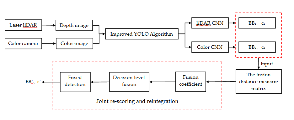
Based on the above analysis, this paper presents a multi-sensor (color camera and LiDAR) and multi-modality (color image and LiDAR depth image) real-time target detection system. Firstly, color image and depth image of the obstacle are obtained using color camera and LiDAR, respectively, and are input into the improved YOLO detection model frame. Then, after the convolution and pooling processing, the detection bounding box for each mode is output. Finally, the two types of detection bounding boxes are fused on the decision-level to obtain the accurate detection target.
In particular, the contributions of this article are as follows:
- (1)
- By incorporating the proposed secondary detection scheme into the algorithm, the YOLO target detection model is improved to detect the targets effectively. Then, decision level fusion is introduced to fuse the image information of LiDAR and color camera output from the YOLO model. Thus, it can improve the target detection accuracy.
- (2)
- The proposed fusion system has been built in related environments, and the optimal parameter configuration of the algorithm has been obtained through training with many samples.
2. System Method Overview
2.1. LiDAR and Color Camera
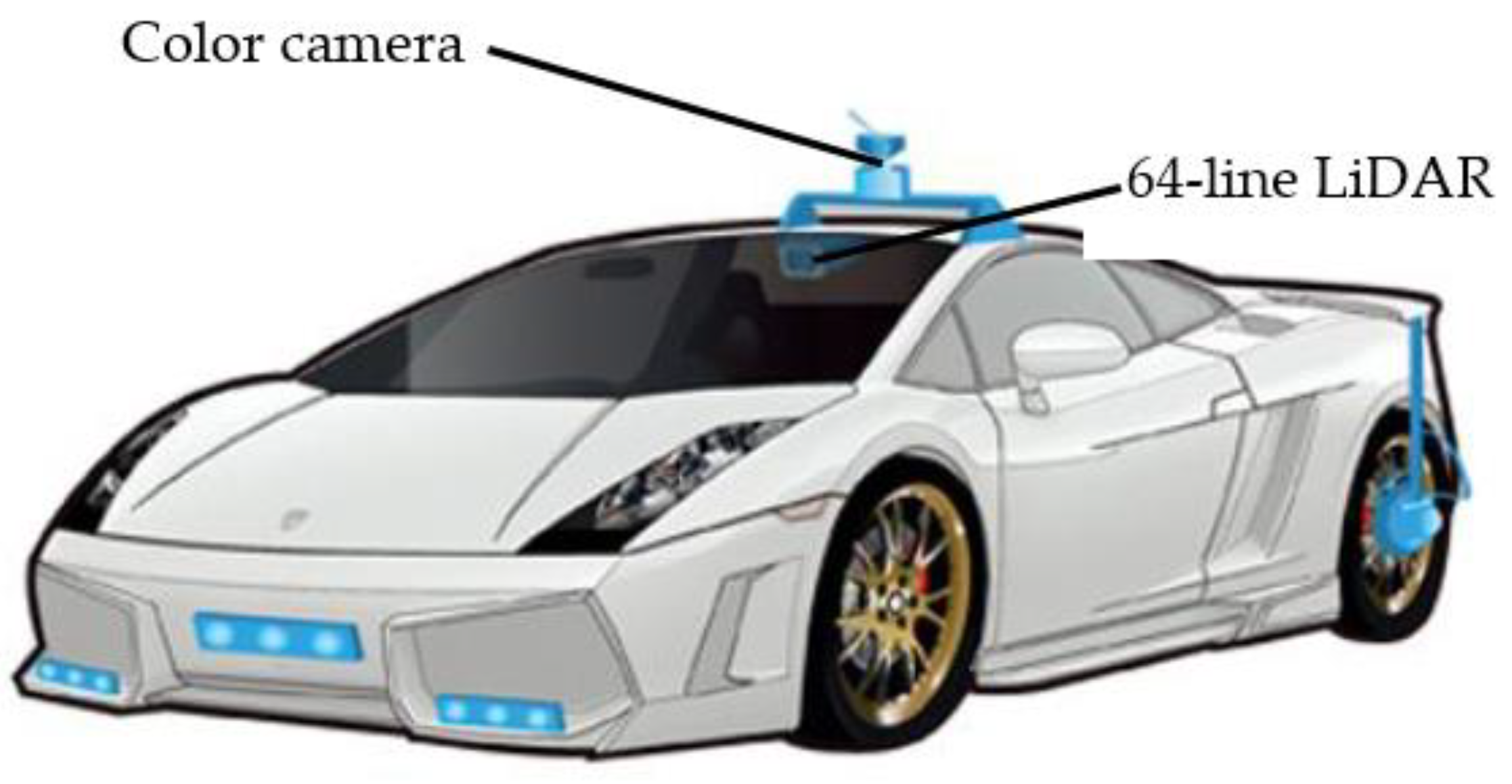
The sensors used in this paper include color camera and LiDAR, as shown in Figure 1.
The LiDAR is a Velodyne (Velodyne LiDAR, San Jose, CA, USA) 64-line three-dimensional radar system which can send a detection signal (laser beam) to a target, and then compare the received signal reflected from the target (the echo of the target) with the transmitted signal. After proper processing, the relevant information of the target can be obtained. The LiDAR is installed at the top center of a vehicle and capable of detecting environmental information through high-speed rotation scanning [11]. The LiDAR can emit 64 laser beams at the head. These laser beams are divided into four groups and each group has 16 laser emitters [12]. The head rotation angle is 360° and the detectable distance is 120 m [13]. The 64-line LiDAR has 64 fixed laser transmitters. Through a fixed pitch angle, it can get surrounding environmental information for each and output a series of three-dimensional coordinate points. Then, the 64 points acquired by the transmitter are marked, and the distance from each point in the scene to the LiDAR is used as the pixel value to obtain a depth image. The color camera is installed under the top LiDAR. The position of the camera is adjusted according to the axis of the transverse and longitudinal center of the camera image and the transverse and longitudinal orthogonal plane formed with the laser projector, so that the camcorder angle and the yaw angle are approximated to 0, and the pitch angle is approximately to 0. Color images can be obtained directly from color cameras, but images output from LiDAR and camera must be matched in time and space to realize the information synchronization of the two.
2.2. Image Calibration and Synchronization
To integrate information in the vehicle environment perceptual system, information calibration and synchronization need to be completed.
2.2.1. Information Calibration
(1) The installation calibration of LiDAR: The midpoints of the front bumper and windshield can be measured with a tape measure, and, according to these two midpoints, the straight line of central axis of the test vehicle can be marked by the laser thrower. Then, on the central axis, a straight line perpendicular to the central axis is marked at a distance of 10 m from the rear axle of the test vehicle; the longitudinal axis of the radar center can be measured by a ruler, and corrected by the longitudinal beam perpendicular to the ground with a laser thrower, to make the longitudinal axis and the beam coincide, and the lateral shift of the radar is approximately 0 m. The horizontal beam of the laser thrower is coincided with the transverse axis of the radar, then the lateral shift of the radar is approximately 0 m.
(2) The installation calibration of camera: The position of the camera is adjusted according to the axis of the transverse and longitudinal center of the camera image and the transverse and longitudinal orthogonal plane formed with the laser projector, so that the camcorder angle and the yaw angle are approximated to 0. Then, the plumb line is used to adjust the pitch angle of the camera to approximately 0.
2.2.2. Information Synchronization
(1) Space matching
Space matching requires the space alignment of vehicle sensors. Assuming that the Velodyne coordinate system is and the color camera coordinate system is , the coordinate system is in translational relationship with respect to the Velodyne coordinate system. The fixing angle between the sensors is adjusted to unify the camera coordinates to the Velodyne coordinate system. Assuming that the vertical height of the LiDAR and color camera is , the conversion relationship of a point “M” in space is as follows:
(2) Time matching
The method of matching in time is to create a data collection thread for the LiDAR and the camera, respectively. By setting the same acquisition frames rate of 30 fps, the data matching on the time is achieved.
2.3. The Process of Target Detection
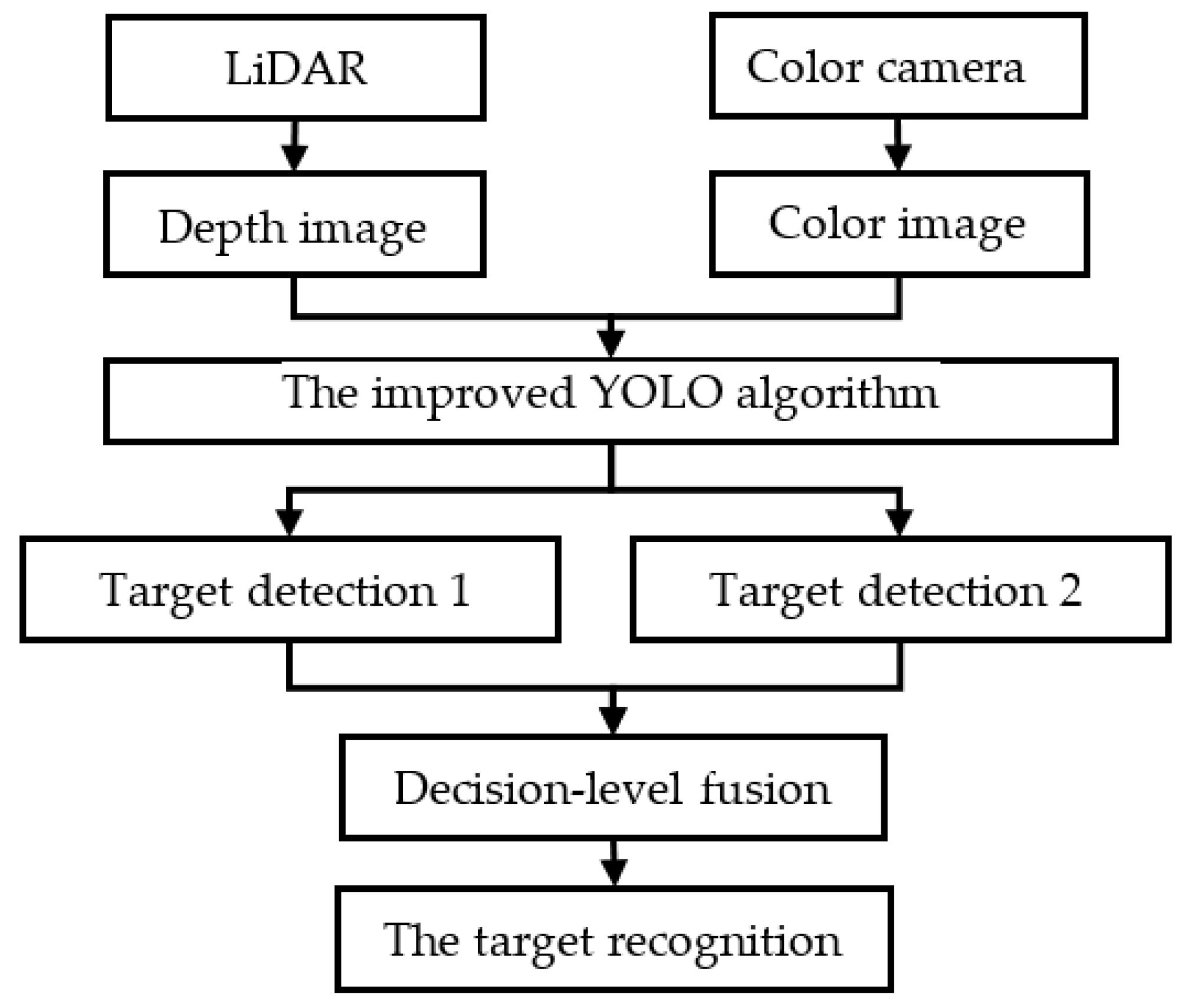
The target detection process based on sensor fusion is shown in Figure 2. After collecting information from the traffic scene, the LiDAR and the color camera output the depth image and the color image, respectively, and input them into the improved YOLO algorithm (the algorithm has been trained by many images collected by LiDAR and color camera) to construct target detection Models 1 and 2. Then, the decision-level fusion is performed to obtain the final target recognition model, which realizes the multi-sensor information fusion.
3. Obstacle Detection Method
3.1. The Original YOLO Algorithm
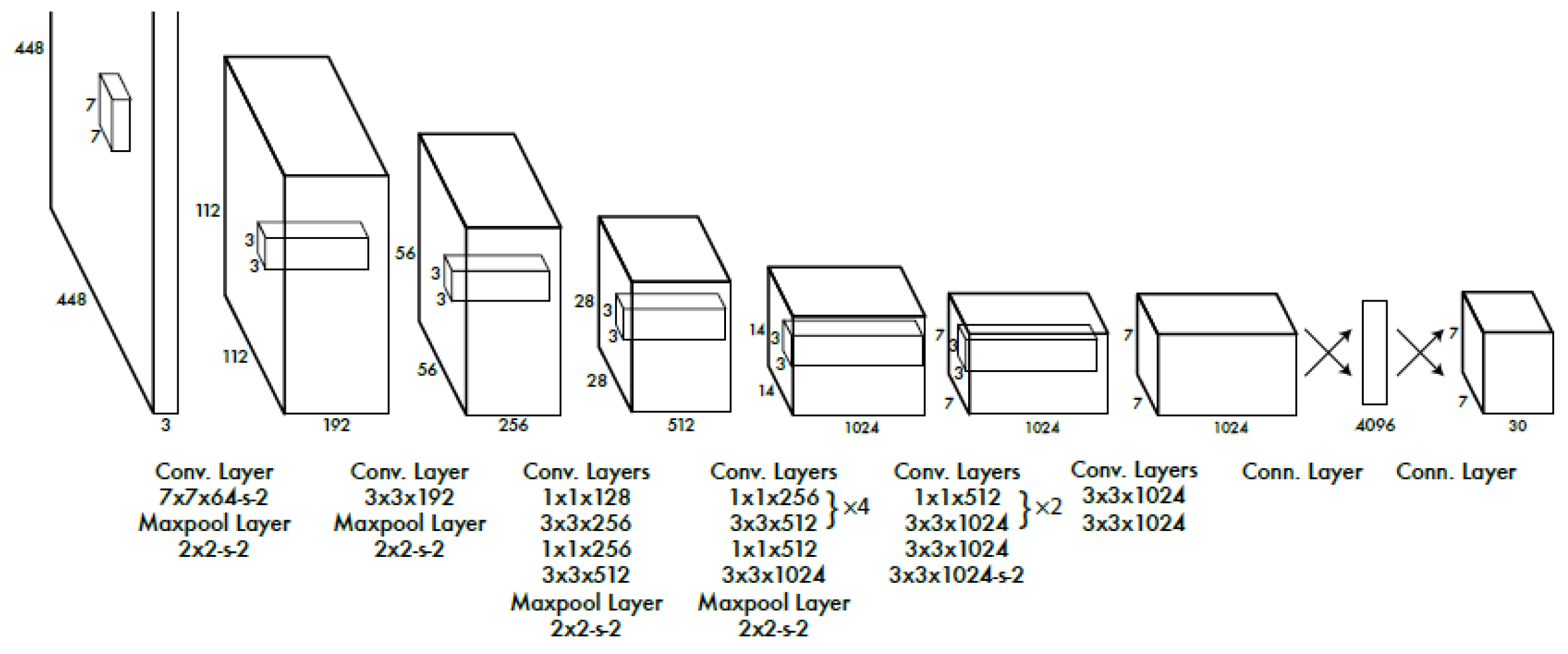
You Only Look Once (YOLO) is a single convolution neural network to predict the bounding boxes and the target categories from full images, which divides the input image into S × S cells and predicts multiple bounding boxes with their class probabilities for each cell. The architecture of YOLO is composed of input layer, convolution layer, pooling layer, fully connected layer and output layer. The convolution layer is used to extract the image features, the full connection layer is used to predict the position of image and the estimated probability values of target categories, and the pooling layer is responsible for reducing the pixels of the slice.
Assume that B is the number of sliding windows used for each cell to predict objects and C is the total number of categories, then the dimensions of output layer is .
The output model of each detected border is as follows:
where represents the center coordinates of the bounding box and represents the height and width of the detection bounding box. The above four indexes have been normalized with respect to the width and height of the image. c is the confidence score, which reflects the probability value of the current window containing the accuracy of the detection object, and the formula is as follows:
where Po indicates the probability of including the detection object in the sliding window, PIOU indicates the overlapping area ratio of the sliding window and the real detected object.
In the formula, BBg is the detection bounding box, and BBg is the reference standard box based on the training label.
For the regression method in the YOLO, the loss function can be calculated as follows:
denotes that the grid cell contains part of the traffic objects. represents the j bounding box in grid cell i. Conversely, represents the j bounding box in grid cell i which does not contain any part of traffic objects. The time complexity of Formula (5) is , which is calculated for one image.
3.2. The Improved YOLO Algorithm
In the application process of the original YOLO algorithm, the following issues are found:
- (1)
- YOLO imposes strong spatial constraints on bounding box predictions since each grid cell only predicts two boxes and can only have one class. This spatial constraint limits the number of nearby objects that our model can predict.
- (2)
- The cell division of the image is set as 7 × 7 in the original YOLO model, which can only detect large traffic objects such as buses, cars and trucks, but does not meet the requirements of cell division of the picture for dim objects such as non-motor vehicles and pedestrians. When the target is close to the safe distance from the autonomous vehicle and the confidence score of the detection target is low, it is easy to ignore the existence of the target to cause security risk.
Based on the above deficiencies, this paper improves the original YOLO algorithm as follows: (1) To eliminate the problem of redundant time caused by the identification of undesired targets, and according to the size and driving characteristics of common targets in traffic scenes, the total number of categories is set to six types, including {bus, car, truck, non-motor vehicle, pedestrian and others}. (2) For the issue of non-motor vehicle and pedestrian detection, this paper proposes a secondary image detection scheme. Then, the cell division of the image is kept as 7 × 7, the sliding window convolution kernel is set as 3 × 3.
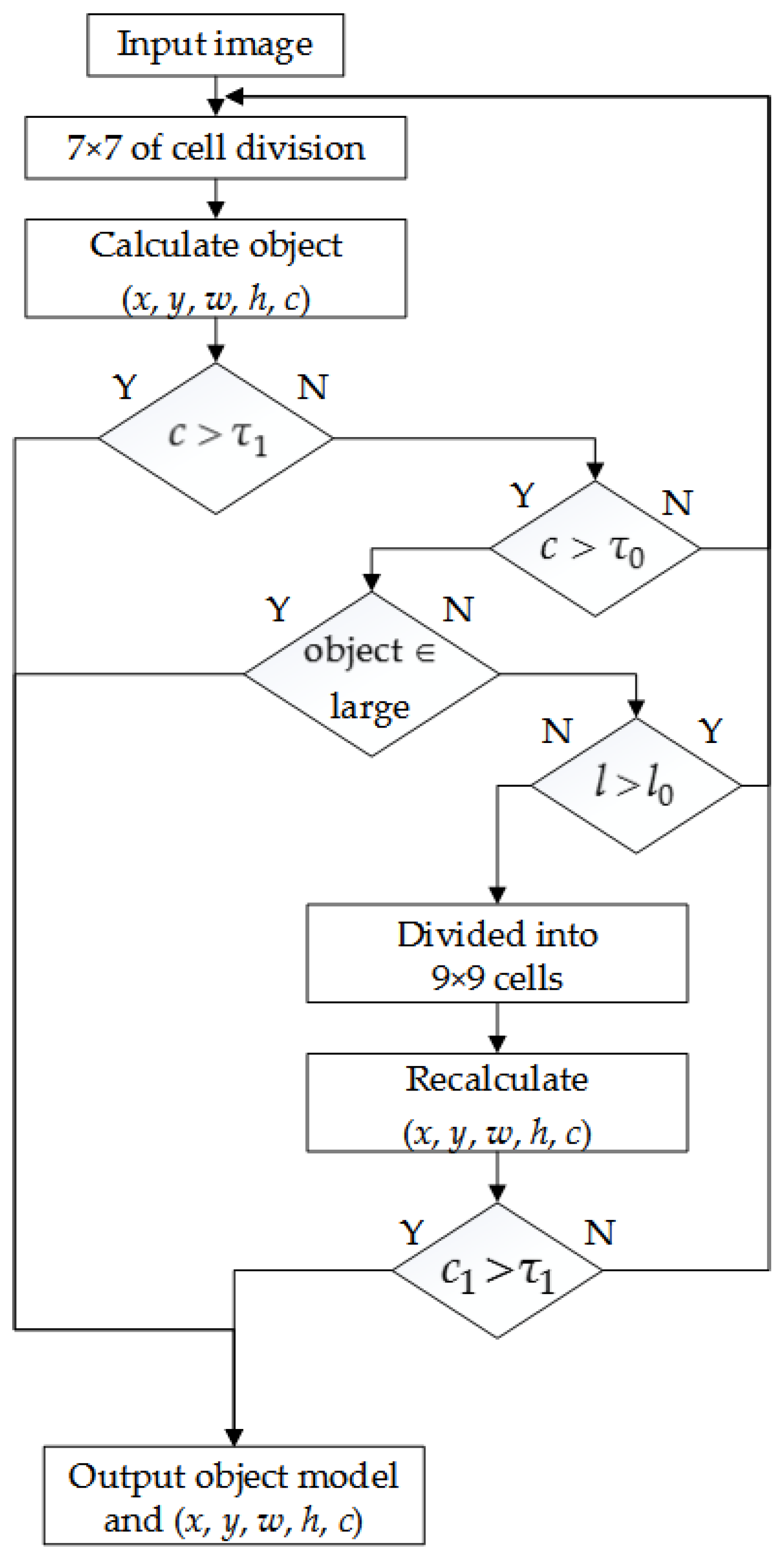
The whole target detection process of the improved YOLO algorithm is shown in Figure 4, and the steps are as follows:
- (1)
- When the target is identified, the confidence score c is higher than the maximum threshold , indicating that the recognition accuracy is high, and the frame model of target detection is directly output.
- (2)
- When the recognition categories are {bus, car and truck}, and the confidence score is ( is the minimum threshold), indicating such targets are large in size and easy to detect, and they can be recognized at the next moment, the current border detection model can be directly output.
- (3)
- When the recognition categories are {non-motor vehicle and pedestrian}, the confidence score is . Due to the dim size and mobility of such targets, it is impossible to accurately predict the position of the next moment. At this time, this target is marked as {others}, indicating that it is required to be detected further. Then, the next steps need to be performed:
- (3a)
- When the distance l between the target marked as {others} and the autonomous vehicle is less than the safety distance l0 (the distance that does not affect decision making; if the distance exceeds it, the target can be ignored), i.e., , the slider region divided as {other} is marked, and the region is subdivided into 9 × 9 cells. The secondary convolution operation is performed again. When the confidence score c of the secondary detection is higher than the threshold , the border model of {others} is output, and the category is changed from {others} to {non-motor vehicle} or {pedestrian}. When the confidence score c of the secondary detection is lower than the threshold , it is determined that the target does not belong to the classification item, and the target is eliminated.
- (3b)
- When , this target is kept as {others}. It does not require a secondary convolution operation.
The original YOLO algorithm fails to distinguish and recognize the targets according to their characteristics, and may lose some targets. The improved YOLO algorithm can try to detect the target twice in a certain distance according to the characteristic of dim of pedestrians and non-motor vehicles. Thus, it is can reduce the missing rate of the target and output a more comprehensive scene model and ensure the safe driving of vehicles.
4. Decision-Level Fusion of the Detection Information
After inputting the depth image and color image into the improved YOLO model algorithm, the detected target frame and confidence score are output, and then the final target model is output based on the fusion distance measurement matrix for decision level fusion.
4.1. Theory of Data Fusion
It is assumed that multiple sensors measure the same parameter, and the data measured by the i sensor and the j sensor are and , and both obey the Gaussian distribution, and their pdf (probability distribution function) curve is used as the characteristic function of the sensor and is denoted as , . and are the observations of and , respectively. To reflect the deviation between and , the confidence distance measure is introduced [15]:
Among them:
The value of is called the confidence distance measure of the i sensor and the j sensor observation, and its value can be directly obtained by means of the error function erf (), namely:
If there are n sensors measuring the same indicator parameter, the confidence distance measure (i, j = 1, 2, ..., n) constitutes the confidence distance matrix of the multi-sensor data:
The general fusion method is to use experience to give an upper bound of fusion, and then the degree of fusion between sensors is:
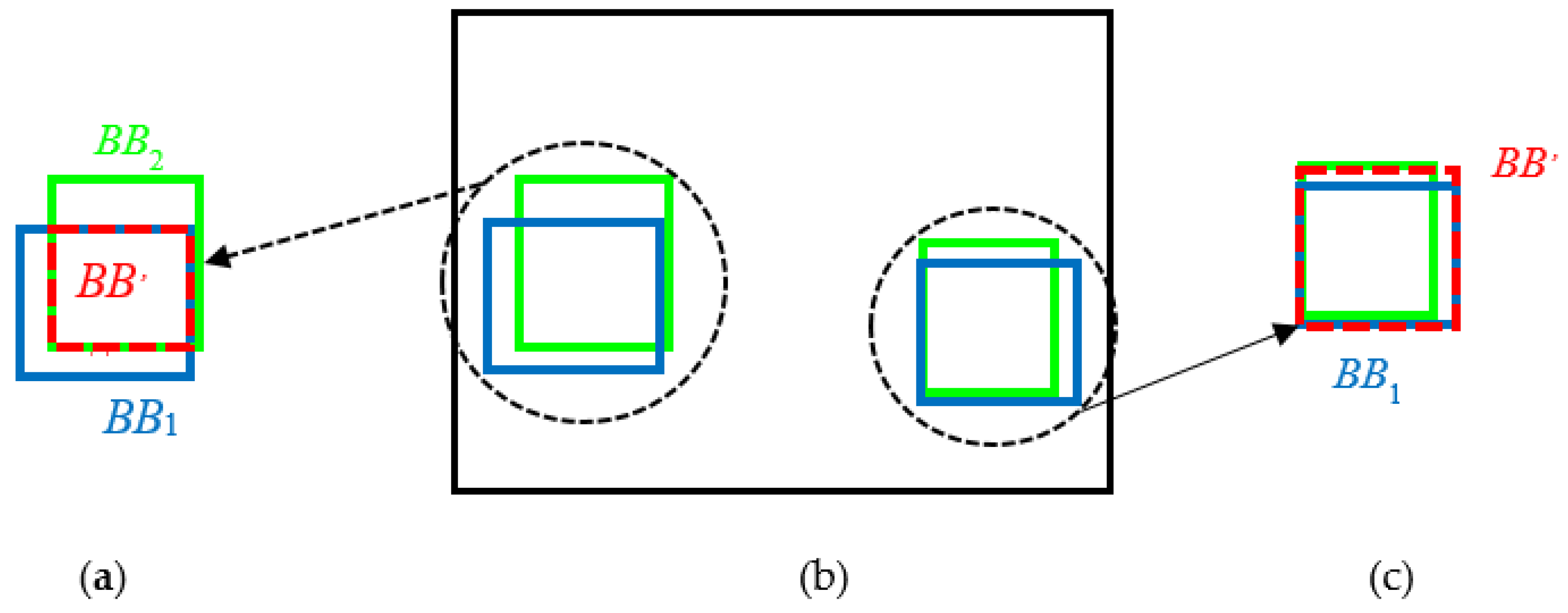
In this paper, there are two sensors, i.e., LiDAR and color camera, so . Then, taking βij = 0.5 [16], r12 is set as the degree of fusion between the two sensors. Figure 5 explains the fusion process.
- (1)
- When r12 = 0, it means that the two sets of border models (green and blue areas) do not completely overlap. At this time, the overlapping area is taken as the final detection model (red area). The fusion process is shown in Figure 5a,b.
- (2)
- When r12 = 1, it indicates that the two border models (green and blue areas) basically coincide with each other. At this time, all border model areas are valid and expanded to the standard border model (red area). The fusion process is shown in Figure 5b,c.
Simple average rules between scores are applied in confidence scores. The formula is as follows:
where c1 is the confidence score of target Model 1, and c2 is the confidence score of target Model 2. In addition, it should be noted that, when there is only one bounding box, to reduce the missed detection rate, this bounding box information is retained as the final output result. The final target detection model can be output through decision-level fusion and confidence scores.
4.2. The Case of the Target Fusion Process
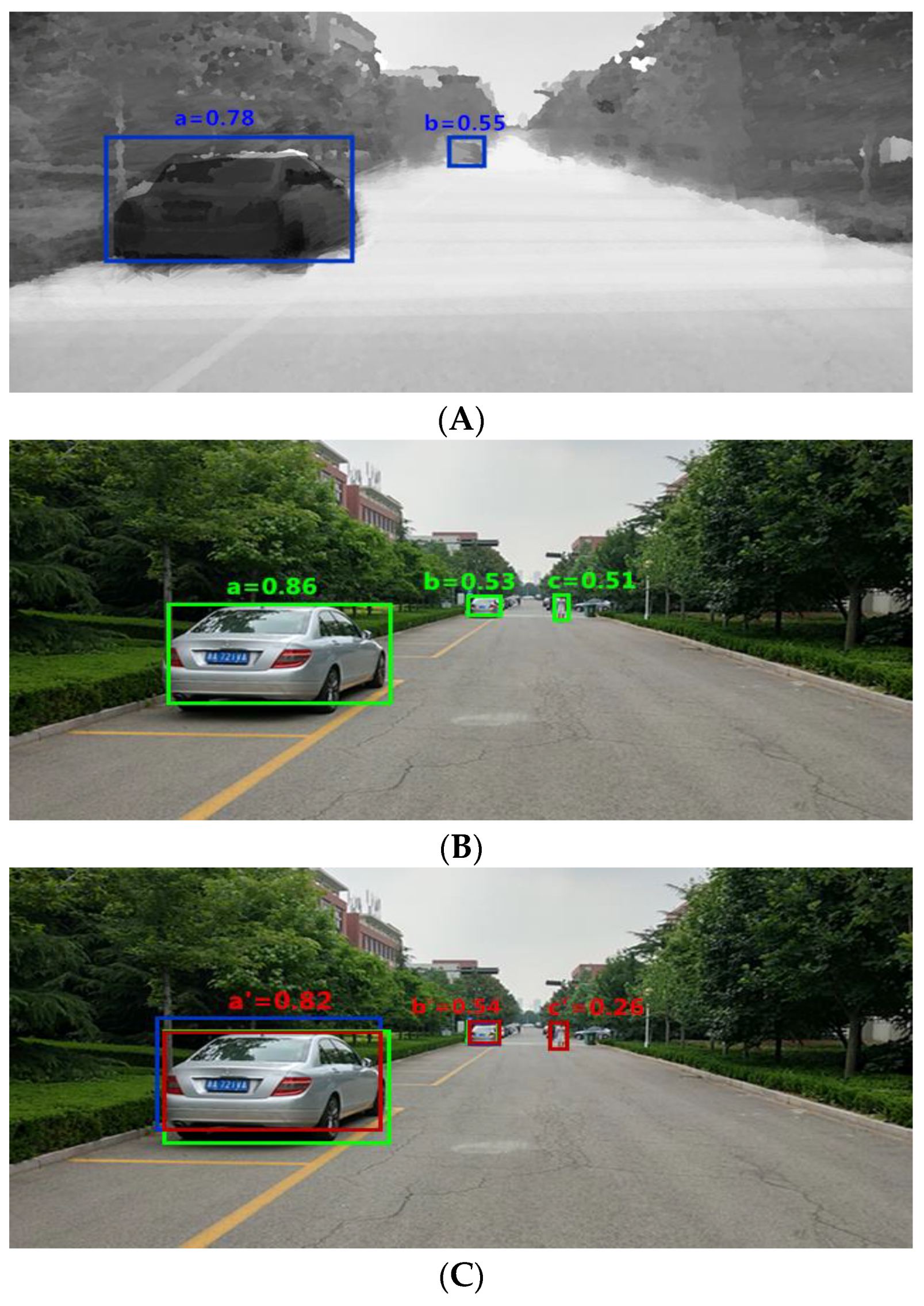
An example of the target fusion process is shown in Figure 6, and the confidence scores obtained using different sensors can be seen in Table 1.
- (1)
- Figure 6A is a processed depth image. It can be seen that the improved YOLO algorithm identifies two targets, a and b, and gives the confidence scores of 0.78 and 0.55, respectively.
- (2)
- Figure 6B is a color image. It can be seen that three targets, a, b, and c, are identified and the confidence scores are given as 0.86, 0.53 and 0.51, respectively.
- (3)
- The red box in Figure 6C is the final target model after fusion:
- (1)
- For target a, according to the decision-level fusion scheme, the result is obtained; then, the overlapping area is taken as the final detection model, and the confidence score after fusion is 0.82, as shown in Figure 6C (a’).
- (2)
- For target b, according to the decision-level fusion scheme, the result is obtained; then, the union of all regions is taken as the final detection model, and the confidence score after fusion is 0.54, as shown in Figure 6C (b’).
- (3)
- For target c, since there is no such information in Figure 6A, and Figure 6B identifies the pedestrian information on the right, according to the fusion rule, the bounding box information of c in Figure 6B is retained as the final output result, and the confidence score is kept as 0.51, as shown in Figure 6C (c’).
5. Results and Discussion
5.1. Conditional Configuration
The target detection training dataset included 3000-frame resolution images of 1500 × 630 and was divided into six different categories: bus, car, truck, non-motor vehicle, pedestrian and others. The dataset was partitioned into three subsets: 60% as training set (1800 observations), 20% as validation set (600 observations), and 20% as testing set (600 observations).
The autonomous vehicles collected data on and off campus. The shooting equipment included a color camera and a Velodyne 64-line LiDAR. The camera was synchronized with a 10 Hz spining LiDAR. The Velodyne has 64-layer vertical resolution, 0.09 angular resolutions, 2 cm of distance accuracy, and captures 100 k points per cycle [9]. The processing platform was completed in the PC segment, including the i5 processor (Intel Corporation, Santa Clara, CA, USA) and GPU (NVIDIA, Santa Clara, CA, USA). The improved YOLO algorithm was accomplished by building a Darket framework and using Python (Python 3.6.0, JetBrains, Prague, The Czech Republic) for programming.
5.2. Time Performance Testing
The whole process included the extraction of depth image and color image, and they were, respectively, substituted into the improved YOLO algorithm and the proposed decision-level fusion scheme as the input layer. The improved YOLO algorithm involved the image grid’s secondary detection process and is therefore slightly slower than the normal recognition process. The amount of computation to implement the different steps of the environment and algorithm is shown in Figure 7. In the figure, it can be seen that the average time to process each frame is 81 ms (about 13 fps). Considering that the operating frequency of the camera and Velodyne LiDAR is about 10 Hz, it can meet the real-time requirements of traffic scenes.
5.3. Training Model Parameters Analysis
The training of the model takes more time, so the setting of related parameters in the model has a great impact on performance and accuracy. Because the YOLO model involved in this article has been modified from the initial model, the relevant parameters in the original model need to be reconfigured through training tests.
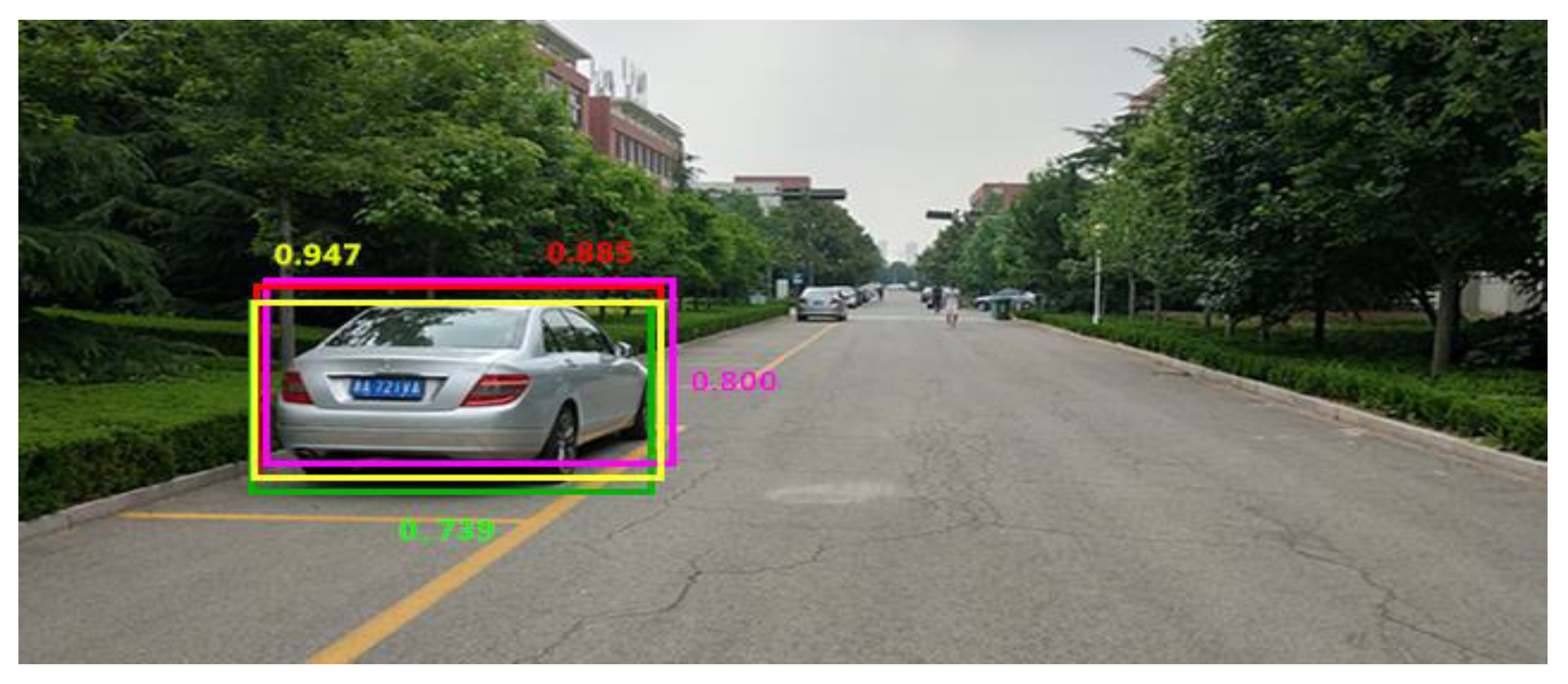
The training step will affect the training time and the setting of other parameters. For this purpose, eight steps of training scale were designed. Under the learning rate of 0.001 given by YOLO, the confidence prediction score, actual score, and recognition time of the model are statistically analyzed. Table 1 shows the performance of the BB2 model, and Figure 7 shows the example results of the BB2 model under D1 (green solid line), D3 (violet solid line), D7 (yellow solid line) and D8 (red solid line).
Table 2 shows that, with the increase of training steps, the confidence score for the BB2 model is constantly increasing, and the actual confidence level is also in a rising trend. When the training step reaches 10,000, the actual confidence score arrives at the highest value of 0.947. However, when the training step reaches 20,000, the actual confidence score begins to fall, and the recognition time also slightly increases, which is related to the configuration of model and the selection of learning rate.
Figure 8 shows the vehicle identification with the training steps of 4000, 6000, 10,000, and 20,000. The yellow dotted box indicates the recognition rate when the learning rate is 10,000. Clearly, the model box basically covers the entire goal and almost no redundant area. Based on the above analysis, the number of steps set in this paper is 10,000.
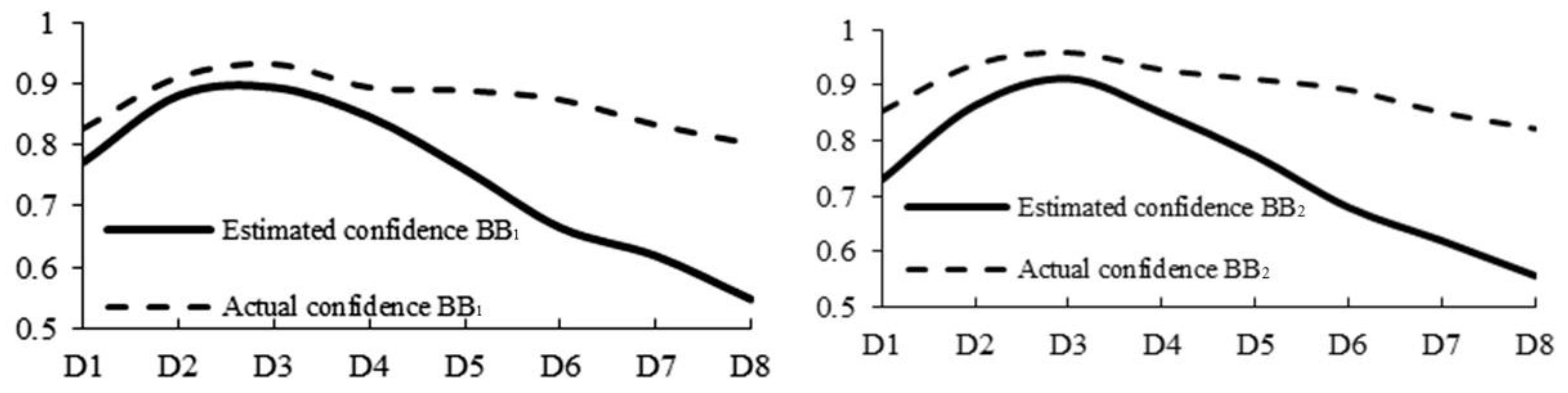
The learning rate determines the speed at which the parameters are moved to the optimal value. To find the optimal learning rate, the model performances with the learning rate of 10−7, 10−6, 10−5, 10−4, 10−3, 10−2, 10−1 and 1 are estimated, respectively, when the training step is set to 10,000.
Table 3 shows the estimated confidence scores and final scores of the output detection models BB1 and BB2 under different learning rates. Figure 9 shows the change trend of the confidence score. After analyzing Table 3 and Figure 9, we can see that, with the decrease of learning rate, all of the confidence prediction score and actual score of model experienced a rising trend firstly and then decreasing. When the learning rate reaches D3 (10−2), the confidence score reaches a maximum value, and the confidence level remains within a stable range with the change of learning rate. Based on the above analysis, when the learning rate is 10−2, the proposed model can obtain a more accurate recognition rate.
5.4. Evaluation of Experiment Results
The paper takes the IOU as the evaluation criteria of recognition accuracy obtained by comparing the BBi (i = 1, 2) of output model and the BBg of actual target model, and defines three evaluation grades:
- (1)
- Low precision: Vehicle targets can be identified within the overlap area, and the identified effective area accounts for 60% of the model total area.
- (2)
- Medium precision: Vehicle targets are more accurately identified in overlapping areas, and the identified effective area accounts for 80% of the model’s total area.
- (3)
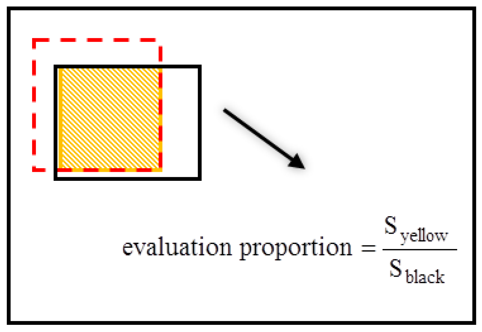
- High precision: The vehicle is accurately identified in the overlapping area, and the identified effective area accounts for 90% of the model total area. Figure 10 is used to describe the definition of evaluation grade. The red dotted frame area is the target actual area and the black frame area is the area BBi output from the model.
To avoid the influence caused by the imbalance of all kinds of samples, the precision and recall were introduced to evaluate the box model under the above three levels:
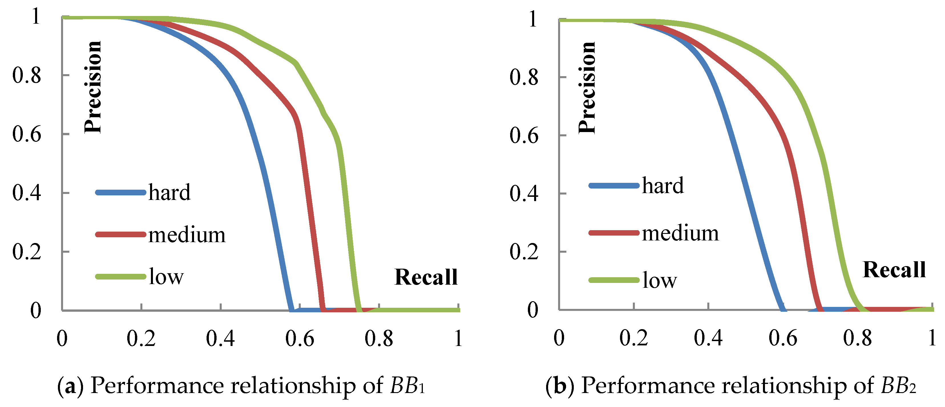
In the formula, TP, FP, and FN indicate the correctly defined examples, wrongly defined examples and wrongly negative examples, respectively. The Precision–Recall diagram for each model BBi (i = 1, 2) is calculated, as shown in Figure 11a,b.
When the recall is less than 0.4, all the accuracy under the three levels is high; when the recall reaches around 0.6, only the accuracy of the level hard decreases sharply and tends to zero, while the accuracy of the other two levels is basically maintained at a relatively high level. Therefore, when the requirements of level for target detection is not very high, the method proposed in this paper can fully satisfy the needs of vehicle detection under real road conditions.
5.5. Method Comparison
The method proposed in this paper is compared with the current more advanced algorithms. The indicators are mainly mAP (mean average precision) and FPS (frames per second). The results obtained are shown in Table 4.
In Table 4, the recognition accuracy of the improved algorithm proposed in this paper is better than that of the original YOLO algorithm. This is related to the fusion decision of the two images and the proposed secondary image detection scheme. To ensure the accuracy, the detection frame number of the improved YOLO dropped from 45 to 13, and the running time increased, but it can fully meet the normal target detection requirements and ensure the normal driving of autonomous vehicles.
6. Conclusions
This paper presents a detection fusion system with integrating LiDAR and color camera. Based on the original YOLO algorithm, the second detection scheme is proposed to improve the YOLO algorithm for dim targets such as non-motorized vehicles and pedestrians. Then, the decision level fusion of sensors is introduced to fuse the color image of color camera and the depth image of LiDAR to improve the accuracy of the target detection. The final experimental results show that, when the training step is set to 10,000 and the learning rate is 0.01, the performance of the model proposed in this paper is optimal and the Precision–Recall performance relationship could satisfy the target detection in most cases. In addition, in the aspect of algorithm comparison, under the requirement of both accuracy and real-time, the method of this paper has better performance and a relatively large research prospect.
Since the samples needed in this paper are collected from several traffic scenes, the coverage of the traffic scenes is relatively narrow. In the future research work, we will gradually expand the complexity of the scenario and make further improvements to the YOLO algorithm. In the next experimental session, the influence of environmental factors will be considered, because the image-based identification method is greatly affected by light. At different distances (0–20 m, 20–50 m, 50–100 m, and >100 m), the intensity level of light is different, so how to deal with the problem of light intensity and image resolution is the primary basis for target detection.
Author Contributions
Conceptualization, J.Z.; Data curation, J.H. and Y.L.; Formal analysis, J.H.; Funding acquisition, S.W.; Investigation, J.H. and J.Z.; Methodology, Y.L.; Project administration, Y.L.; Resources, J.H.; Software, J.Z.; Supervision, J.Z. and S.W.; Validation, S.W.; Visualization, Y.L.; Writing—original draft, J.H.; and Writing—review and editing, J.Z., S.W. and S.L.
Funding
This work was financially supported by the National Natural Science Foundation of China under Grant No. 71801144, and the Science & Technology Innovation Fund for Graduate Students of Shandong University of Science and Technology under Grant No. SDKDYC180373.
Conflicts of Interest
The authors declare no conflict of interest.
References
- Batch Re-normalization of Real-Time Object Detection Algorithm YOLO. Available online: http://www.arocmag.com/article/02-2018-11-055.html (accessed on 10 November 2017).
- Liu, Y.; Zhang, Y.; Zhang, X. Adaptive spatial pooling for image classification. Pattern Recognit. 2016, 55, 58–67. [Google Scholar] [CrossRef]
- Gao, Z.; Li, S.B.; Chen, J.N.; Li, Z.J. Pedestrian detection method based on YOLO network. Comput. Eng. 2018, 44, 215–219, 226. [Google Scholar]
- Improved YOLO Feature Extraction Algorithm and Its Application to Privacy Situation Detection of Social Robots. Available online: http://kns.cnki.net/kcms/detail/11.2109.TP.20171212.0908.023.html (accessed on 12 December 2017).
- Nguyen, V.T.; Nguyen, T.B.; Chung, S.T. ConvNets and AGMM Based Real-time Human Detection under Fisheye Camera for Embedded Surveillance. In Proceedings of the 2016 International Conference on Information and Communication Technology Convergence (ICTC), Jeju, South Korea, 19–21 October 2016; pp. 840–845. [Google Scholar]
- Azim, A.; Aycard, O. Detection, Classification and Tracking of Moving Objects in a 3D Environment. In Proceedings of the IEEE Intelligent Vehicles Symposium, Alcala de Henares, Spain, 3–7 June 2012; pp. 802–807. [Google Scholar]
- Zhou, J.J.; Duan, J.M.; Yang, G.Z. A vehicle identification and tracking method based on radar ranging. Automot. Eng. 2014, 36, 1415–1420, 1414. [Google Scholar]
- Asvadi, A.; Premebida, C.; Peixoto, P.; Nunes, U. 3D Lidar-based static and moving obstacle detection in driving environments: An approach based on voxels and multi-region ground planes. Robot. Auton. Syst. 2016, 83, 299–311. [Google Scholar] [CrossRef]
- Asvadi, A.; Garrote, L.; Premebida, C.; Peixoto, P.; Nunes, U.J. Multimodal Vehicle Detection: Fusing 3D-LIDAR and Color Camera Data. Pattern Recognit. Lett. 2017. [Google Scholar] [CrossRef]
- Xue, J.R.; Wang, D.; Du, S.Y. A vision-centered multi-sensor fusing approach to self-localization and obstacle perception for robotic cars. Front. Inf. Technol. Electron. Eng. 2017, 18, 122–138. [Google Scholar] [CrossRef]
- Wang, X.Z.; Li, J.; Li, H.J.; Shang, B.X. Obstacle detection based on 3d laser scanner and range image for intelligent vehicle. J. Jilin Univ. (Eng. Technol. Ed.) 2016, 46, 360–365. [Google Scholar]
- Glennie, C.; Lichti, D.D. Static calibration and analysis of the Velodyne HDL-64E S2 for high accuracy mobile scanning. Remote Sens. 2010, 2, 1610–1624. [Google Scholar] [CrossRef]
- Yang, F.; Zhu, Z.; Gong, X.J.; Liu, J.L. Real-time dynamic obstacle detection and tracking using 3D lidar. J. Zhejiang Univ. 2012, 46, 1565–1571. [Google Scholar]
- Zhang, J.M.; Huang, M.T.; Jin, X.K.; Li, X.D. A real-time Chinese traffic sign detection algorithm based on modified YOLOv2. Algorithms 2017, 10, 127. [Google Scholar] [CrossRef]
- Han, F.; Yang, W.H.; Yuan, X.G. Multi-sensor Data Fusion Based on Correlation Function and Fuzzy Clingy Degree. J. Proj. Rocket. Missiles Guid. 2009, 29, 227–229, 234. [Google Scholar]
- Chen, F.Z. Multi-sensor data fusion mathematics. Math. Pract. Theory 1995, 25, 11–15. [Google Scholar]
- Redmon, J.; Divvala, S.; Girshick, R.; Farhadi, A. You Only Look Once: Unified, Real-Time Object Detection. In Proceedings of the IEEE Conference on Computer Vision and Pattern Recognition, Las Vegas, NV, USA, 27–30 June 2016; pp. 779–788. [Google Scholar]
- Girshick, R. Fast R-CNN. In Proceedings of the 2015 IEEE International Conference on Computer Vision (ICCV), Santiago, Chile, 7–13 December 2015; pp. 1440–1448. [Google Scholar]
- Ren, S.; He, K.; Girshick, R. Faster R-CNN: Towards real-time object detection with region proposal networks. Int. Conf. Neural Inf. Process. Syst. 2015, 39, 91–99. [Google Scholar] [CrossRef] [PubMed]
- Wei, P.; Cagle, L.; Reza, T.; Ball, J.; Gafford, J. LiDAR and camera detection fusion in a real-time industrial multi-sensor collision avoidance system. Electronics 2018, 7, 84. [Google Scholar] [CrossRef]
- Li, B. 3D fully convolutional network for vehicle detection in point cloud. arXiv, 2017; arXiv:1611.08069. [Google Scholar]
- Voting for Voting in Online Point Cloud Object Detection. Available online: Https://www.researchgate.net/publication/314582192_Voting_for_Voting_in_Online_Point_Cloud_Object_Detection (accessed on 13 July 2015).
Figure 1.
Installation layout of two sensors.

Figure 2.
The flow chart of multi-modal target detection.

Figure 3.
The YOLO network architecture. The detection network has 24 convolutional layers followed by two fully connected layers. Alternating 1 × 1 convolutional layers reduce the features space from preceding layers. We pre-train the convolutional layers on the ImageNet classification task at half the resolution (224 × 224 input images) and then double the resolution for detection.

Figure 4.
The flow chart of secondary image detection program. Object large means that targets are {bus, car, truck}.
Figure 4.
The flow chart of secondary image detection program. Object large means that targets are {bus, car, truck}.

Figure 5.
Decision-level fusion diagram of detection model. Blue area (BB1) is the model output from the depth image. Green area (BB2) is the model output from the color image. Red area (BB’) is the final detection model. When r12 = 0, the fusion process is shown in (a). The models not to be fused are shown in (b). When r12 = 1, the fusion process is shown in (c).

Figure 6.
An example of target detection fusion process. (A) is a processed depth image. The models detected a and b are shown with blue. (B) is a color image. The models detected a, b and c are shown with green. (C) is the final target model after fusion. The models fused a’, b’ and c’ are shown with red.

Figure 7.
Processing time for each step of the inspection system (in ms).

Figure 8.
Performance comparison of BB2 model under 4 kinds of training steps.

Figure 9.
Performance trends under different learning rates.

Figure 10.
The definition of evaluation grade. The yellow area is the identified effective area. The black frame area is model’s total area. The above proportion is the ratio between yellow area and black area.
Figure 10.
The definition of evaluation grade. The yellow area is the identified effective area. The black frame area is model’s total area. The above proportion is the ratio between yellow area and black area.

Figure 11.
Detection performance of the target. (A) is the performance relationship of model BB1. (B) is the performance relationship of model BB2.
Figure 11.
Detection performance of the target. (A) is the performance relationship of model BB1. (B) is the performance relationship of model BB2.


Table 1.
Confidence scores obtained using different sensors.
| Sensor | Confidence Score (Detected Object from Left to Right) | ||
|---|---|---|---|
| a (a’) | b (b’) | c (c’) | |
| LiDAR | 0.78 | 0.55 | -- |
| Color camera | 0.86 | 0.53 | 0.51 |
| The fusion of both | 0.82 | 0.54 | 0.26 |
Table 2.
Performance of BB2 model under different steps.
| Mark | Number of Steps | Estimated Confidence | Actual Confidence | Recognition Time (ms) |
|---|---|---|---|---|
| D1 | 4000 | 0.718 | 0.739 | 38.42 |
| D2 | 5000 | 0.740 | 0.771 | 38.40 |
| D3 | 6000 | 0.781 | 0.800 | 38.33 |
| D4 | 7000 | 0.825 | 0.842 | 38.27 |
| D5 | 8000 | 0.862 | 0.885 | 38.20 |
| D6 | 9000 | 0.899 | 0.923 | 38.12 |
| D7 | 10,000 | 0.923 | 0.947 | 38.37 |
| D8 | 20,000 | 0.940 | 0.885 | 38.50 |
Table 3.
Model performance under different learning rates.
| Mark | Learning Rate | Estimated Confidence | Actual Confidence | ||
|---|---|---|---|---|---|
| BB1 | BB2 | BB1 | BB2 | ||
| D1 | 1 | 0.772 | 0.73 | 0.827 | 0.853 |
| D2 | 10−1 | 0.881 | 0.864 | 0.911 | 0.938 |
| D3 | 10−2 | 0.894 | 0.912 | 0.932 | 0.959 |
| D4 | 10−3 | 0.846 | 0.85 | 0.894 | 0.928 |
| D5 | 10−4 | 0.76 | 0.773 | 0.889 | 0.911 |
| D6 | 10−5 | 0.665 | 0.68 | 0.874 | 0.892 |
| D7 | 10−6 | 0.619 | 0.62 | 0.833 | 0.851 |
| D8 | 10−7 | 0.548 | 0.557 | 0.802 | 0.822 |
© 2018 by the authors. Licensee MDPI, Basel, Switzerland. This article is an open access article distributed under the terms and conditions of the Creative Commons Attribution (CC BY) license (http://creativecommons.org/licenses/by/4.0/).
Share and Cite
MDPI and ACS Style
Han, J.; Liao, Y.; Zhang, J.; Wang, S.; Li, S. Target Fusion Detection of LiDAR and Camera Based on the Improved YOLO Algorithm. Mathematics 2018, 6, 213. https://doi.org/10.3390/math6100213
AMA Style
Han J, Liao Y, Zhang J, Wang S, Li S. Target Fusion Detection of LiDAR and Camera Based on the Improved YOLO Algorithm. Mathematics. 2018; 6(10):213. https://doi.org/10.3390/math6100213
Chicago/Turabian StyleHan, Jian, Yaping Liao, Junyou Zhang, Shufeng Wang, and Sixian Li. 2018. "Target Fusion Detection of LiDAR and Camera Based on the Improved YOLO Algorithm" Mathematics 6, no. 10: 213. https://doi.org/10.3390/math6100213
Note that from the first issue of 2016, this journal uses article numbers instead of page numbers. See further details here.