A Within-Host Stochastic Model for Nematode Infection


1
Instituto de Ciencias Matemáticas CSIC-UAM-UC3M-UCM, Calle Nicolás Cabrera 13-15, 28049 Madrid, Spain
2
Department of Applied Mathematics, School of Mathematics, University of Leeds, Leeds LS2 9JT, UK
*
Author to whom correspondence should be addressed.
Mathematics 2018, 6(9), 143; https://doi.org/10.3390/math6090143
Submission received: 25 June 2018
/
Revised: 6 August 2018
/
Accepted: 11 August 2018
/
Published: 21 August 2018
(This article belongs to the Special Issue Stochastic Processes with Applications)
Abstract
:We propose a stochastic model for the development of gastrointestinal nematode infection in growing lambs under the assumption that nonhomogeneous Poisson processes govern the acquisition of parasites, the parasite-induced host mortality, the natural (no parasite-induced) host mortality and the death of parasites within the host. By means of considering a number of age-dependent birth and death processes with killing, we analyse the impact of grazing strategies that are defined in terms of an intervention instant , which might imply a move of the host to safe pasture and/or anthelmintic treatment. The efficacy and cost of each grazing strategy are defined in terms of the transient probabilities of the underlying stochastic processes, which are computed by means of Strang–Marchuk splitting techniques. Our model, calibrated with empirical data from Uriarte et al and Nasreen et al., regarding the seasonal presence of nematodes on pasture in temperate zones and anthelmintic efficacy, supports the use of dose-and-move strategies in temperate zones during summer and provides stochastic criteria for selecting the exact optimum time instant when these strategies should be applied.
1. Introduction
Gastrointestinal (GI) nematodes are arguably (see [1,2]) the major cause of ill health and poor productivity in grazing sheep worldwide, especially in young stock. Productivity losses result from both parasite challenge and parasitism, while regular treatment of the infections is costly in terms of chemicals and labour. The relative cost of GI parasitism has become greater in recent decades as the availability of effective broad-spectrum anthelmintics (see Chapter 5 of [1]) has enabled the intensification of pastoral agriculture. To an extent, it appears the success of the various anthelmintic products developed since the 1960s has created a rod for our own backs, particularly as resistance has arisen to each active family in turn (see, for example, [3,4]). Options for the control of GI nematode infections (which do not rely uniquely on the use of anthelmintics) include management procedures (involving intervention with anthelmintics, grazing management, level of nutrition and bioactive forages), biological control (with nematophagous fungi), selection for genetic resistance in sheep (within breed/use of selected breeds) and vaccination. The article by Stear et al. [5] gives an overview of alternatives to anthelmintics for the control of nematodes in livestock, and it complements and extends other review articles by Hein et al. [6], Knox [7], Sayers and Sweeney [8] and Waller and Thamsborg [9]. Moreover, we refer the reader to the article by Smith et al. [10] for stochastic and deterministic models of anthelmintic resistance emergence and spread.
The aim of this paper is to present a stochastic model for quantitatively comparing among various grazing strategies involving isolation, movement or treatment of the host, but without incorporating the risk of selecting for resistance. This amounts to the assumption that the nematodes in our model have not been previously exposed to the anthelmintic treatments under consideration; see, for example, [11]. We point out that the effect of the resistance in the dynamics is usually limited by the rotation of different anthelmintic classes on an annual basis (see [12,13]).
A wide range of mathematical models can be found in the literature for modelling the infection dynamics of nematodes in ruminants. Originally, simple deterministic models were proposed in terms of systems of ordinary differential equations describing the population dynamics of infected ruminants and nematodes on pasture. By describing these dynamics in a deterministic way, the resulting models were tractable from a mathematical and analytical point of view [14]. However, efforts were soon redirected towards stochastic approaches given the importance of stochastic effects in these systems [15]. These stochastic effects are related to, among others, spatial dynamics, clumped infection events or individual heterogeneities related to the host’s immune response to infection [16]. Without any aim of an exhaustive enumeration, we refer the reader to [15,17,18] for deterministic and stochastic models of nematode infection in ruminants for a population of hosts maintaining a fixed density.
In this paper, we develop a mathematical model for the within-host GI nematode infection dynamics, to compare the effectiveness and cost of various worm control strategies, which are related to pasture management practices and/or strategic treatments based on the use of a single anthelmintic drug. Control criteria are applied to the development of GI nematode parasitism in growing lambs. Specifically, the interest is in the parasite Nematodirus spp. with Nematodirus battus, Nematodirus filicollis and Nematodirus spathiger as the main species. The resulting grazing management strategies are specified in terms of an intervention instant that, under certain specifications, implies moving animals to safe pastures and/or anthelmintic treatment. For a suitable selection of , we present two control criteria that provide a suitable balance between the efficacy and cost of intervention. Our methodology is based on simple stochastic principles and time-dependent continuous-time Markov chains; see the book by Allen [19] for a review of the main results for deterministic and stochastic models of interacting biological populations.
Our work in this paper is directly related to that in [20], where we examine stochastic models for the parasite load of a single host and where the interest is in analysing the efficacy of various grazing management strategies. In [20], we defined control strategies based on isolation and treatment of the host at a certain age . This means that the host is free living in a seasonal environment, and it is transferred to an uninfected area at age . In the uninfected area, the host does not acquire new parasites, undergoes an anthelmintic treatment to decrease the parasite load and varies in its susceptibility to parasite-induced mortality and natural (no parasite-induced) mortality. From a mathematical point of view, an important feature of the analysis in [20] is that the underlying processes, recording the number of parasites infesting the host at an arbitrary time t, can be thought of as age-dependent versions of a pure birth process with killing and a pure death process with killing, which are both defined on a finite state space.
Here, we complement the treatment of control strategies applied to GI nematode burden that we started in [20] by focusing on strategies that are not based on isolation of the host; to be concrete, our interest is in three grazing strategies that reflect the use of a paddock with safe pasture and/or the efficacy of an anthelmintic drug. Seasonal fluctuations in the acquisition of parasites, the death of parasites within the host and the natural and parasite-induced host mortality are incorporated into our model by using nonhomogeneous Poisson processes. Contrary to [20], grazing management strategies considered in this work lead to, instead of pure birth/death processes with killing, the analysis of several age-dependent birth and death processes with killing. The efficacy and cost of each grazing strategy are defined in terms of the transient probabilities of each of the underlying stochastic processes; that is, the probability that the parasite load of the infected host is at any given level at each time instant, given that a particular control strategy has been applied at the intervention instant . In order to compute these probabilities, we apply Strang–Marchuk splitting techniques for solving the corresponding systems of differential equations.
The paper is organized as follows. In Section 2, we define the mathematical model used in various grazing management strategies, derive the analytical solution of the underlying time-dependent systems of linear differential equations and present two criteria allowing us to find the instant that appropriately balances effectiveness and cost of intervention in these grazing strategies. In Section 3, we examine seasonal changes of GI nematode burden in growing lambs. Finally, concluding remarks are given in Section 4.
2. Stochastic Within-Host Model and Control Criteria
In this section, we first propose a mathematical stochastic model for the within-host infection dynamics by GI nematodes in growing lambs, define grazing management strategies and set down a set of equations governing the dynamics of the underlying processes. We then present control criteria based on stochastic principles. For the sake of brevity, we refer the reader to Appendix A where we comment on the equivalence used in Table 1 of [20] in the identification of the degree of infestation, level of infection, eggs per gram (EPG) value, number of infective larvae in the small intestine and the points system. Further details on the taxonomy and morphology of the parasite Nematodirus spp. and the treatment and control of parasite gastroenteritis in sheep can be found in [1,2,21].
2.1. Grazing Management Strategies: A Stochastic Within-Host Model
We define the mathematical model in terms of levels of infection and let the random variable record the infection level of the host at time t. From Table 1 of [20], this means that the degree of infestation is null if , light if with , moderate if with , high if with and heavy if . In the setting of GI nematode parasitism, the value amounts to a critical level that does not permit the host to develop immunity to the nematode infection, in such a way that an eventual intervention is assumed to be ineffective as the degree of infestation is heavy. Therefore, we let be equivalent to the degree heavy of infestation (i.e., the number of infective larvae in the small intestine is greater than 12,000 worms) or the death of the host. Let denote the set of infection levels, with .
We consider individual-based grazing strategies, which are related to a single lamb (host) that is born, parasite-free, at time and, over its lifetime, is exposed to parasites at times that form a nonhomogeneous Poisson process of rate . At every exposure instant, the host acquires parasites, independently of one exposure to another. It is assumed that the number of acquired parasites does not allow the level of infection to increase more than one unit at any acquisition instant, which is a plausible assumption in our examples where increments in the number of infective larvae in the small intestine are registered at daily intervals. Let be the death rate of the host at age t in the absence of any parasite burden, and assume that this rate is increased by an amount , which is related to the parasite-induced host mortality as the infection level equals m at age t. For later use, we define the functions and for levels , where denotes Kronecker’s delta.
At age , the interest is in the level of infection as, under certain grazing assumptions, intervention is prescribed at a certain age . Note that the host at age can be dead or its degree of infestation can be heavy (), and it can be alive and parasite-free (), or it can be alive and infected ( with ).
In analysing the process , we distinguish between the free-living interval and the post-intervention interval ; for ease of presentation, we first digress to briefly recall the analytic solution for ages given in [20]. For a host that has survived at age t with , the infection dynamics within the host are analysed in terms of transient probabilities , for levels . That is, represents the probability of the host being at infection level m at time t. These dynamics lead us to a pure birth process with killing on the state space (see Figure 1 in [20]), the age-dependent birth and killing rates of which are given by and , respectively, for , and where is an absorbing state. Expressions for can be then evaluated following our arguments in Section 2.2 of [20].
Next, we focus on three grazing strategies that are defined in terms of the intervention instant . This implies that, at post-intervention ages , the rates , and are replaced by functions , and , respectively, allowing us to show concrete effects of an intervention on the lamb and its environmental conditions. To be concrete, the functions , and appropriately reflect the use of a paddock with safe pasture and/or the efficacy of an anthelmintic treatment, in accordance with the following grazing strategies:
- Strategy UM:
- The host is left untreated, but moved to a paddock with safe pasture at age . The resulting process can be thought of as an age-dependent pure birth process with killing, the birth rates of which are given by if , and if , and killing rates are defined by if and if , for .
- Strategy TS:
- The host is treated with anthelmintics and set-stocked at age . Let be the death rate of parasites when the infection level of the host is at time t with . In this case, can be seen as an age-dependent birth and death process with killing. The birth and death rates are defined by if , if and if , for , respectively. Killing rates are defined identically to the rates in strategy UM.
- Strategy TM:
- The host is treated with anthelmintics and moved to safe pasture at age . In a similar manner to strategy TS, the process may be formulated as an age-dependent birth and death process with killing. Birth, death and killing rates are identical to those in strategy TS with the exception of for time instants , which has the form .
In strategies TS and TM, a single anthelmintic drug is used. In accordance with the empirical data in [22], resistance is not incorporated into modelling aspects since year is assumed in Section 3. The resulting models are thus related to the rotation of different anthelmintic classes on an annual basis, which has been widely promoted and adopted as a strategy to delay the development of anthelmintic resistance in nematode parasites; see, e.g., [12,13].
For the sake of completeness, we introduce the term scenario US to reflect no intervention, that is the host is left untreated and set-stocked. Note that, in such a case, the process is an age-dependent pure birth process with killing, and its birth and killing rates are specified by and if , for . It follows then that the transient distribution of is readily derived from [20] for time instants .
A slight modification of our arguments in solving Equations (1) and (2) of [20] allows us to derive explicit expressions for the transient solution at post-intervention instants in grazing strategy UM. For time instants , we introduce the probability of the process being at infection level m at time t, given that strategy UM is implemented at the intervention instant , and initial conditions , for . Then, the transient solution at time instants can be readily expressed as:
where and . Starting from:
the functions , for values , are iteratively computed as:
with .
2.2. Splitting Techniques
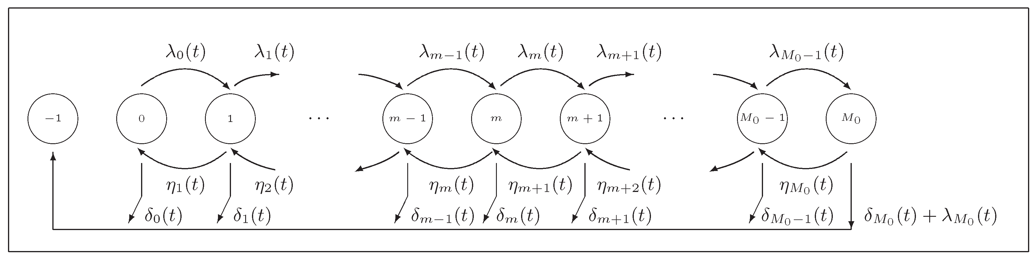
For grazing strategies TS and TM, the transient solution at time instants can be numerically derived by using splitting techniques; see [23]. In a unifying manner, we may observe that, for a host that has survived at age t with and , the possible transitions (in both strategies TS and TM) are as follows (Figure 1):
- (i)
- at rate , for levels ;
- (ii)
- at rate , for levels ;
- (iii)
- at rate , for levels ;
- (iv)
- at rate .
Then, if we select a certain grazing strategy s with , the resulting probabilities , for and time instants , satisfy the equality:
and the time-dependent linear system of differential equations:
where , and is a tridiagonal matrix with entries:
Needless to say, initial conditions in Equation (2) are given by where the values for with do not depend on the grazing strategy under consideration.
In principle, the system (2) of differential equations could be solved in many ways, but Strang–Marchuk splitting techniques are concretely used in Section 3 to derive its solution. Following the approach in [23], the original problem given by Equation (2) is first split into several subsystems that are then solved cyclically one after the other. This procedure is particularly advisable when tailor-made numerical methods can be applied for each split subsystem or when, as occurs in our case, explicit solutions for the subsystems can be derived.
The approach in Section 1.3 of [23] is of particular interest when, for a certain splitting , the time-dependent linear systems of differential equations:
can be accurately and efficiently solved, which is our case here. In our examples in Section 3, we consider the splitting with:
and we evaluate numerically the transient solution at time instants by solving a sequence of four time-dependent linear subsystems of differential equations.
In order to determine the probabilities for levels and a certain grazing strategy s with , we first select the splitting time-step as with , and introduce the notation:
At step n with , we solve the subsystems , , and cyclically on successive intervals of length , using the solution of one subsystem as the initial condition of the other one as follows:
This procedure results in the solution at , which is given by since . Then, we may proceed similarly in the numerical evaluation of the transient solution at subsequent time instants with and , by replacing by in (3) and (4), so that the solution of the previous subsystems at time instant is now used as the initial condition in the subsystem at step . We refer the reader to [23] for qualitative properties of the operator splitting approach and convergence order.
For grazing strategy , the entries , for levels , of the vector are given by Equation (1) for time instants , with replaced by , and the function replaced by in the case TS.
The solution at time instants has entries:
where and, starting from:
the functions , for values , can be iteratively evaluated as:
with .
2.3. Control Criteria Based on Stochastic Principles
For grazing strategies UM, TS and TM, we define a control strategy by means of an age and an intervention rule, which is related to a concrete infection level and the resulting probability:
This age-dependent probability allows us to determine a set of potential intervention instants satisfying the inequality for a predetermined index ; note that in the case regardless of the threshold .
It should be pointed out that, in grazing strategies UM and TM, maintaining safe-pasture conditions in a paddock for the whole year does not seem feasible in practice. Moreover, treating the host with anthelmintic drugs (cases TS and TM) within early days of the year will not yield optimal results, since profits of treatment cannot be obtained before host exposure to infection; see Figure A1 in Appendix A. Thus, we focus on values in such a way that, for a fixed pair with , those instants can be seen as either low-risk (states ) or extreme-risk () intervention instants, and consequently, they are not taken into account in our next arguments.
In carrying out our examples, we select the threshold yielding a moderate degree of infestation (according to Table 1 of [20]) and the index . Then, for each resulting set of potential intervention instants, the problem is to find a single instant that appropriately balances the effectiveness and cost of intervention in the grazing strategy under consideration. In our approach, the effectiveness and cost functions can be seen as alternative measures of the efficacy of an intervention, with a negative significance in the case of the cost function. To be concrete, in an attempt to reflect the effect of the parasite burden on the lamb weight at age , effectiveness is measured in terms of:
which corresponds to the probability that the degree of infestation at age is null or light as the intervention is prescribed at age in accordance with the grazing strategy s with . In contrast, we make the cost of intervention depend on the probability:
that either the host does not survive or its degree of infestation is high at age . It is worth noting that operational (financial) costs are not considered within the modelling framework, which will allow us to derive a single intervention instant regardless of concrete specifications for the cost of maintaining safe-pasture conditions, or the cost of purchasing the anthelmintic drugs. Then, the proposed cost function , which can be seen as a negative measure of efficacy, is related to productivity losses corresponding to high levels of infection, and it may be advisable when the financial fluctuations (in comparing various drugs, how prices of anthelmintics change) over time are not known in advance.
For a suitable choice of , the following control criteria are suggested:
- Criterion 1:
- We select the intervention instant verifying , where the subset consists of those potential intervention instants satisfying the inequality , for a certain probability .
- Criterion 2:
- We select the intervention instant such that , where the subset is defined by those time instants verifying , for a certain probability .
Our objective in Criterion 1 is thus to minimize the cost of intervention and to maintain a minimum level of effectiveness, which is translated into the probability . In Criterion 2, the objective is to maximize the effectiveness and to set an upper bound to the cost of intervention. An alternative manner to measure the effectiveness and cost of intervention at a certain age is given by the respective values:
where if in scenario US and if , and if in grazing strategy s with ; then, values for and are related to the expected proportions of time that the degree of infestation is either null or light, and either high or heavy, respectively.
3. Empirical Data, Age-Dependent Rates and Results
Age-dependent patterns are from now on specified to reflect that the parasite-induced death of the host is negligible, and death rates in the absence of any parasite burden at free-living instants and post-intervention instants are identical, that is for levels . Nevertheless, we point out that, in a general setting, the analytical solution in Equations (1) and (2) allows and to be potentially different from and , respectively, and it can be therefore applied when, among other circumstances, maintaining identical environmental conditions at free-living and post-intervention instants is not possible (i.e., different rates and ) and/or anthelmintic resistance must be considered within the modelling framework (i.e., different functions and ). In our examples, we select = , from which it follows that the probability that, in absence of any parasite burden, the host dies in the interval with year equals , and the conditional probability that the host death occurs within the first 24 hours, given that it dies in the interval , equals .
In Section 3.1, the age-dependent rates and defining grazing strategies UM, TS and TM are inherently connected to the empirical data in [24] and Figure 2 of [22]. To be concrete, we first use the results in Section 3.2 of [20] to specify the function for time instants in scenario US and for time instants in grazing strategies UM, TS and TM. Concrete specifications for age-dependent patterns at time instants are then derived by suitably modifying these functions under the distributional assumptions in the cases UM, TS and TM. Results yielding scenario US are related to the study conducted by Uriate et al. [22], which was designed to describe monthly fluctuations of nematode burden in sheep (Rasa Aragonesa female lambs) raised under irrigated conditions in Ebro Valley, Spain, by using worm-free tracer lambs and monitoring the faecal excretion of eggs by ewes. Specifically, the age-dependent rate for ages in scenario US and grazing strategy TS and ages in the cases UM and TM is obtained by following our arguments in Section 3.2 of [20]. Therefore, the function is related to increments in the number of infective larvae in the small intestine of the lamb (Figure 2, Figure 3 and Figure 4, shaded area), and it is computed as a function of the infection levels in Table 1 of [20]. To reflect the use of safe pasture in grazing strategies UM and TM, it is assumed that for ages , where denotes the previously specified function, which is linked to the original paddock. In grazing strategies TS and TM, the empirical data in [22] are appropriately combined with those data in [24] on the clinical efficacy assessment of ivermectin, fenbendazole and albendazole in lambs parasited with nematode infective larvae; similarly to Section 3.2 in [20], the death rates of parasites in the cases TS and TM are then given by , for levels , where reflects the chemotherapeutic efficacy of a concrete anthelmintic over time. More details on the specific form of and can be found in Appendix A.
3.1. Preliminary Analysis
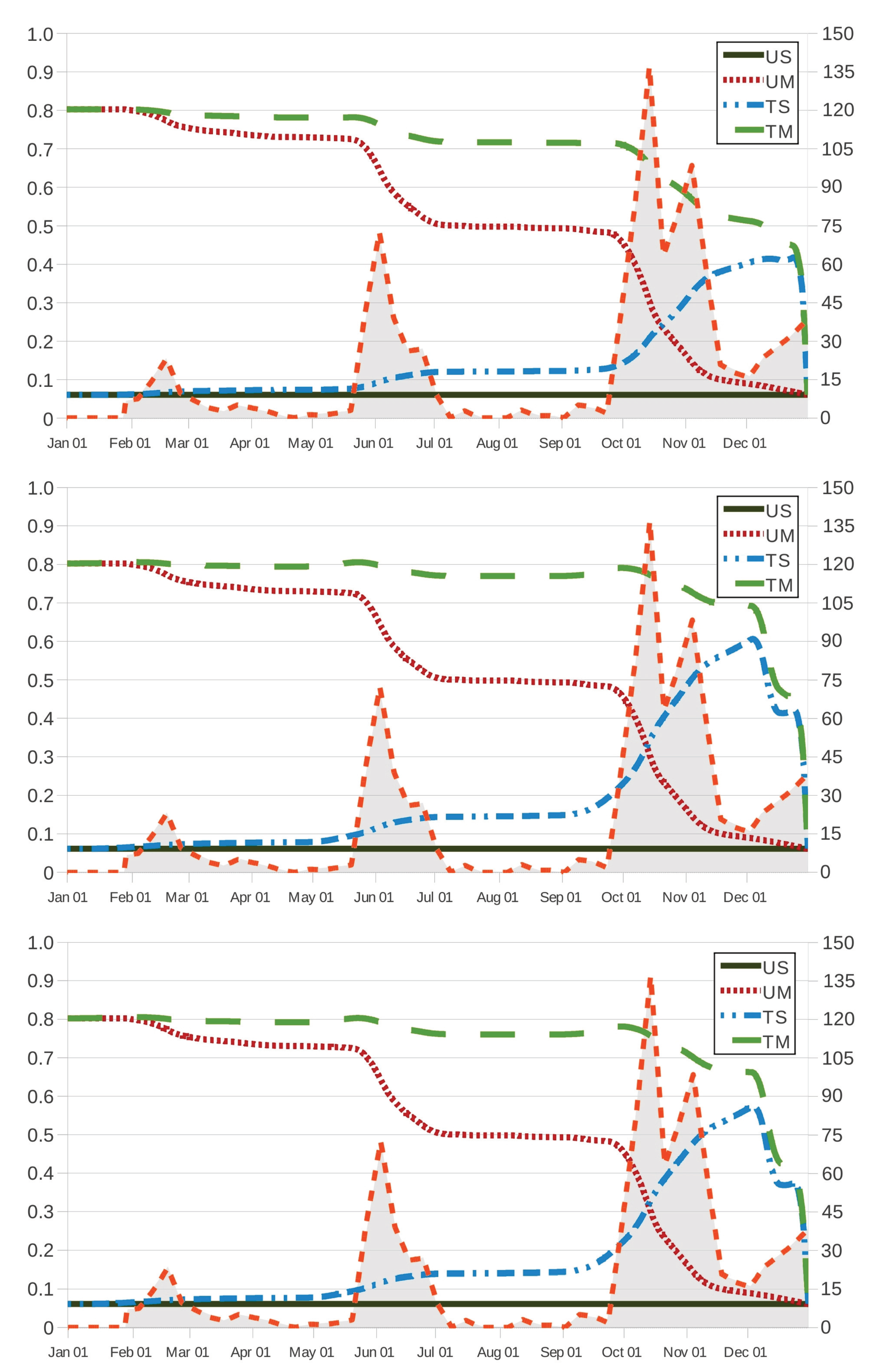
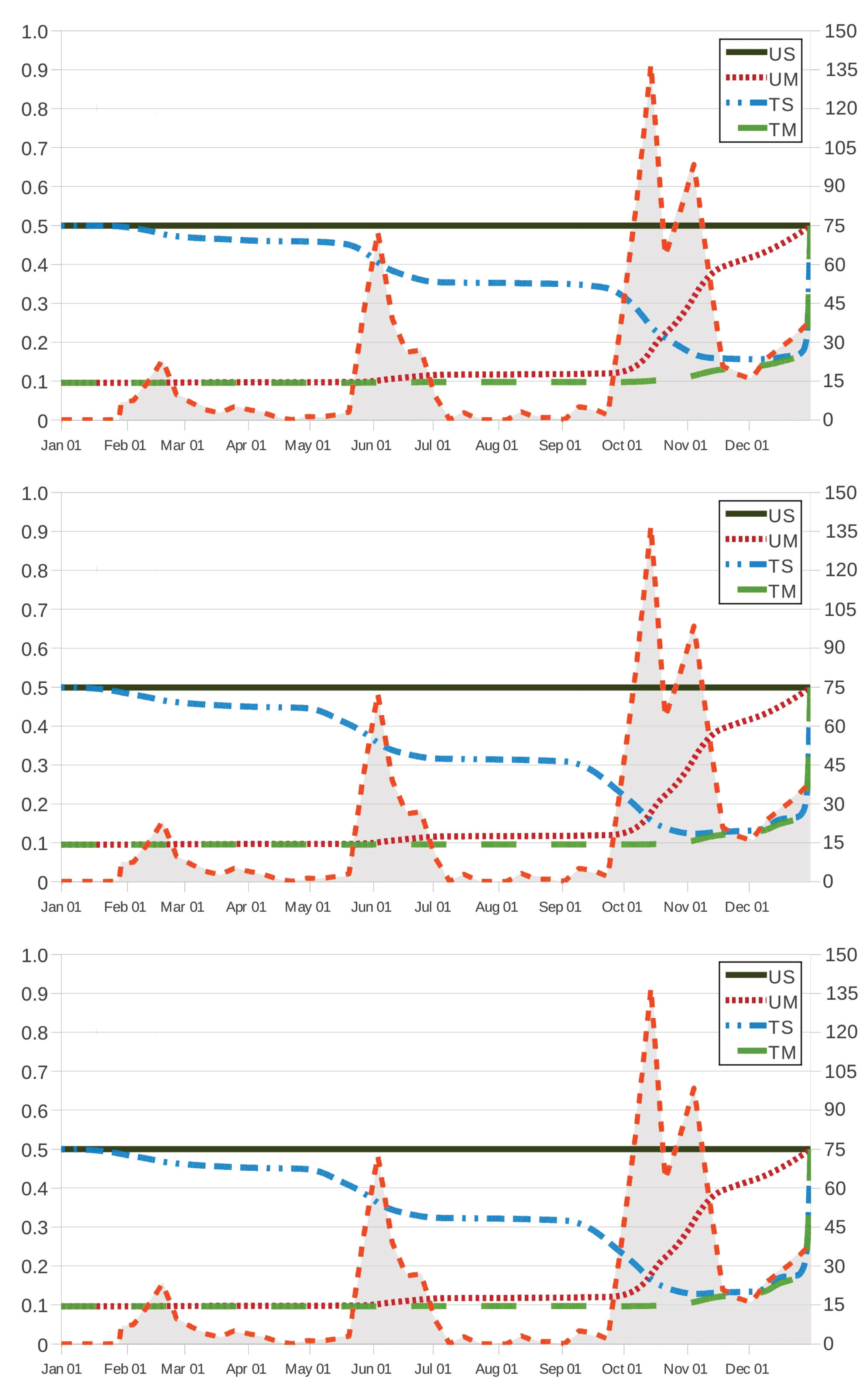
Because of seasonal conditions, a preliminary analysis of the probabilities and in the cases UM, TS and TM is usually required to determine values and in such a way that Criteria 1 and 2 lead us to non-empty subsets and of potential intervention instants , for a predetermined threshold . A graphical representation of and can help in measuring allowable values for the minimum value of effectiveness and the maximum cost of intervention in terms of concrete values for and , respectively. Figure 2 and Figure 3 show how and behave in terms of for grazing strategies UM, TS and TM. We remark here that, in scenario US, the effectiveness (respectively, cost of intervention) is given by (respectively, ), which is a constant as a function of . It is worth noting that the value (respectively, ) results in a lower bound (respectively, upper bound) to the corresponding values of effectiveness (respectively, cost of intervention) in grazing strategies UM, TS and TM.
The effectiveness and cost functions for strategies UM and TM are monotonic in one direction, while the corresponding curves for strategy TS are largely in the opposite direction. This corroborates that an early movement of the host to safe pasture results in a more effective (Figure 2) and less expensive (Figure 3) solution regardless of other actions on the use of anthelmintic drugs, which is related to the safe-pasture conditions having less free-living than the original paddock. On the contrary, set-stocking conditions made an early intervention seem inadvisable and, due to the effect of the therapeutic period (28 days), intervention should be prescribed by the end of November in the case TS.
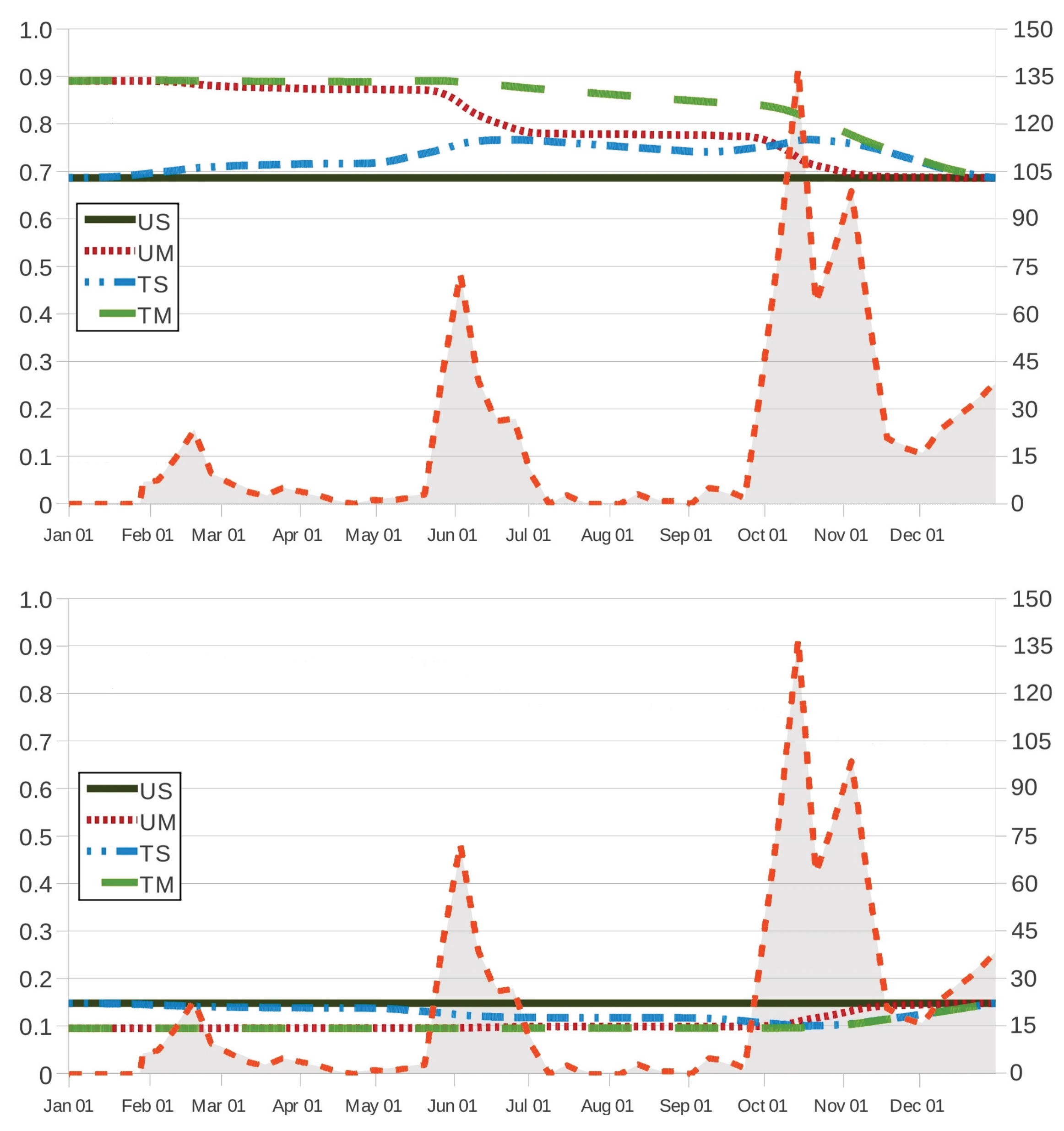
As intuition tells us, grazing strategy TM results in the most effective procedure for every time instant , regardless of the anthelmintic treatment. In Figure 2 and Figure 3, it is also seen that grazing strategy UM is preferred to grazing strategy TS when intervention is prescribed at ages (21 October), 285 (13 October) and 286 (14 October) as the respective anthelmintics ivermectin, fenbendazole and albendazole are used in the case TS; on the contrary, the latter is preferred to the former at intervention instants , 285 and 286. This behaviour is also noted in Figure 4, where we make the effectiveness and cost of intervention amount to and , respectively; in such a case, grazing strategy UM is preferred to grazing strategy TS for intervention instants (6 October) as the host is treated with fenbendazole, and the latter is preferred to the former in the case of intervention instants (9 October). For grazing strategy TS, it is seen in Figure 2 (respectively, Figure 3) that the effectiveness function (respectively, the cost function ) appears to behave as an increasing (respectively, decreasing) function of the intervention instant as (13 December) and 338 (5 December) if the anthelmintic ivermectin and the anthelmintics fenbendazole and albendazole are administered to the host (respectively, (6 November), 308 (5 November) and 339 (6 December) if anthelmintics ivermectin, fenbendazole and albendazole are used); moreover, its variation over time seems to be more apparent, in agreement with three periods of maximum pasture contamination, with kg DM (by mid-February), kg DM (by 2 June) and kg DM (between October and November) as maximum values of infective larvae on herbage. Figure 2 (respectively, Figure 3) allows us to remark that, in comparison with the case TS, these periods of maximum pasture contamination influence in an opposite manner the effectiveness (respectively, cost of intervention) in grazing strategies UM and TM.
3.2. Intervention Instants
In Table 1, we list the value of the effectiveness and the cost of intervention for certain intervention instants derived by applying Criteria 1 and 2 in grazing strategies UM, TS and TM, for probabilities and and a variety of values of the index p; in scenario US, effectiveness and cost are replaced by the probabilities and , respectively. A detailed discussion on the instants in Table 1 and some related consequences can be found in Appendix A.2. It can be noticed that the selection (1 October), which is related to the index in the case TM with the anthelmintic fenbendazole, results in the minimum cost of intervention (0.09589, instead of 0.49951 in scenario US) and the maximum effectiveness (0.79086, instead of 0.06072 in scenario US), and it can be thus taken as optimal for our purposes. Moreover, the anthelmintic fenbendazole is found the most effective drug since the highest values of and the smallest values of are observed in Table 1 for every grazing strategy and fixed intervention instant .
Values for and in Table 1 correspond to the expected proportions of time that the host infection level remains in the subsets of levels and , respectively. It is remarkable to note that the maximum effectiveness (instead of 0.68645 in scenario US) and the minimum cost of intervention (instead of 0.14746 in scenario US) are both related to the selection (19 June) in grazing strategy TM with the anthelmintic ivermectin. It should be noted that results in the longest post-intervention interval in our examples; similarly to the case of control strategies based on isolation and anthelmintic treatment of the host (see Section 3.3 in [20]), the maintenance of stable safe-pasture conditions for a long period of time may often be difficult and highly expensive, so that the choice might be unsustainable for practical use.
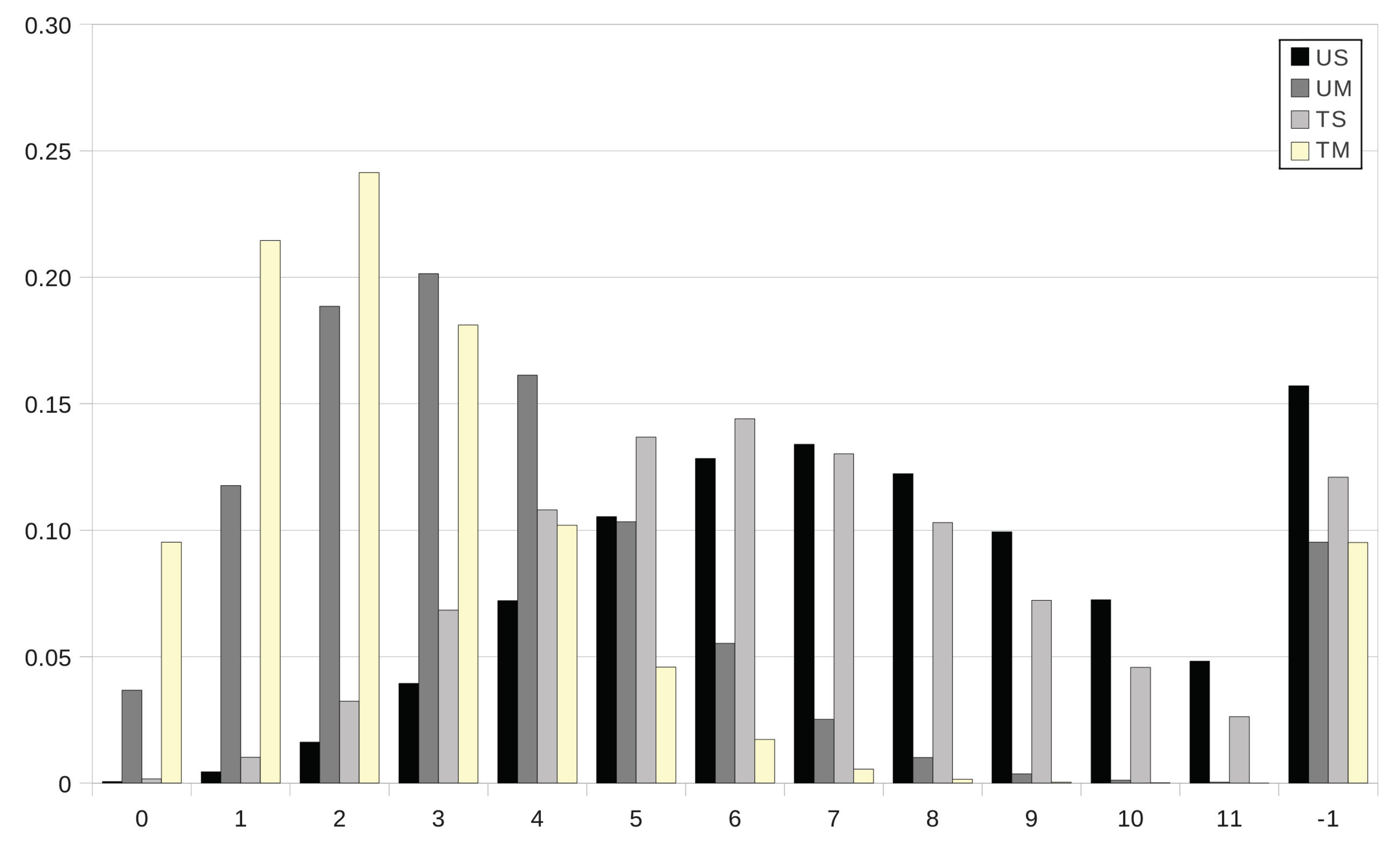
An interesting question concerns the comparative analysis between the mass functions of the parasite burden at age year in grazing strategies UM, TS and TM and the corresponding mass function in the case of no intervention. In Figure 5, we first focus on this question as intervention is prescribed at age in grazing strategies UM, TS and TM, with the anthelmintic drug ivermectin in the cases TS and TM. The movement of the host to safe pasture (strategies UM and TM) at day yields a significant decrease in the probability that the host does not survive at age year ( and in the cases UM and TM, respectively, instead of in scenario US), as well as an important decrease in the expected degree of infestation in the case of survival; more particularly, the degree of infestation is expected to be light as either anthelmintic drugs are used () or the host is transferred to a paddock with safe pasture (), instead of moderate and nearly high in the case US (). Set-stocking conditions are not as effective as the movement of the host to safe pasture since the expected degree of infestation amounts to a moderate degree in the case of survival (); moreover, for grazing strategy TS, the decrease in the probability of no-survival is apparent, but it is not as notable as for strategies UM and TM. In Figure 6, we plot the mass function of the parasite burden at age year in scenario US versus its counterpart in grazing strategy TM, when animals are treated with ivermectin, fenbendazole and albendazole at ages , 273 and 272, respectively. By Table A2 and Table A3 in Appendix A, ages , 273 and 272 are all feasible intervention instants, which leads us to mass functions that are essentially comparable in magnitude. On the contrary, the shape and magnitudes of the mass function in grazing strategy TM are dramatically different from the shape and magnitudes in scenario US, where no intervention is prescribed, irrespective of the anthelmintic product.
4. Conclusions
It is of fundamental importance in the development of GI nematode infection in sheep to understand the role of grazing management in reducing anthelmintic use and improving helminth control. With empirical data of [22,24], we present a valuable modelling framework for better understanding the host-parasite interaction under fluctuations in time, which arguably represents the most realistic setting for assessing the impact of seasonal changes in the parasite burden of a growing lamb. Grazing strategies UM, TS and TM in Section 2.1 are defined in terms of an eventual movement to safe pasture and/or chemotherapeutic treatment of the host at a certain age . For a suitable choice of , we suggest to use two control criteria that adequately balance the effectiveness and cost of intervention at age by using simple stochastic principles. Specifically, each intervention instant in Table 1 yields an individual-based grazing strategy for a lamb that is born, parasite-free, at time (1 January, in our examples). The individual-based grazing strategies UM, TS and TM can be also thought of as group-based grazing strategies in the case of a flock consisting of young lambs, essentially homogeneous in age. In such a case, intervention at age is prescribed (in accordance with a predetermined grazing strategy) by applying our methodology to a typical lamb that is assumed to be born, parasite-free, at a certain average day . Then, results may be routinely derived by handling the set of empirical data in Figure 2 in [22] starting from day , instead of Day 0, since intervention at time instant amounts to age of the typical lamb in the paddock. From an applied perspective, the descriptive model in Section 2 becomes a prescriptive model as the set of empirical data in Figure 2 in [22] is appropriately replaced by a set of data derived by taking the average of annual empirical data from historical records.
For practical use, the profits of applying Criteria 1 and 2 in grazing strategies UM, TS and TM should be appropriately compared with experimental results. To that end, we first comment on general guidelines (see Part II of [25]) for control of GI nematode infection. From an experimental perspective, the dose-and-move strategy (termed TM) is usually recommended in mid-July, this recommendation being applicable in temperate zones where the maximum numbers of infective larvae do not occur before midsummer, which is our case (Figure 2, Figure 3 and Figure 4, shaded area). As stated in [25], midsummer movement to safe pasture without deworming (strategy UM) is thought of as a low cost control measure; it can even be effective at moderate levels of pasture infectivity, and it has the advantage of creating no anthelmintic resistance by drug selection. We may translate these specifications into an intervention at day (15 July) in strategies TM and UM. Guidelines for the application of an anthelmintic drug without movement (strategy TS) are not so clearly available, and various alternatives (based mainly on the several-dose approach) are applied in a variety of circumstances that strongly depend on the geographical region, climate and farming system. For comparative purposes in strategy TS, we compare our results (derived by applying Criteria 1 and 2) with an intervention at day (15 October), when the maximum number of infective larvae on herbage is observed (Figure 2, Figure 3 and Figure 4, shaded area).
We present in Table 2 a sample of our results when the anthelmintic fenbendazole is used in grazing strategies TS and TM. Table 2 lists values of the reduction in the mean infection level (RMIL) at age year, under the taboo that the host survives at age year, and the reduction in the total lost probability (RTLP) when, instead of scenario US, intervention is prescribed at day by a certain grazing strategy s with . The indexes RMIL and RTLP for grazing strategy s, with , are defined by:
where denotes the conditional expected infection level of the host at age year, given that it survives at age year, and is the probability that the host does not survive at age year, when intervention is prescribed at day according to grazing strategy s. The values and are related to scenario US, and they reflect no intervention.
In grazing strategies UM and TM, the experimental selection (midsummer) is found to be near an optimal solution, and Table 2 permits us to analyse the effects of the stochastic control criteria in a more detailed manner. Based on the decreasing monotonic behaviour of RMIL and RTLP with respect to the intervention instant , it is noticed that the later we apply grazing strategies UM and TM, the worse the results we obtain. This is closely related to the important role played in the cases UM and TM by the use of safe pasture, which is reflected in the contamination reduction with respect to the original paddock. Therefore, the movement of the host to safe pasture appears to be dominant in the use of anthelmintics, so that the sooner the host is moved, the safer it is for the host. The maintenance of stable safe-pasture conditions for a long period of time may be difficult and/or highly expensive, whence additional considerations should be taken into account when selecting the time instant for moving the host. In grazing strategy UM, the intervention instant should be considered as optimal for our purposes, and it yields a reduction of in the mean infection level at the end of the year, as well as a reduction of in the probability of no-survival. However, an intervention at day (i.e., moving the host to safe pasture more than one hundred days later) would result in significantly lower operational costs, but predicted reductions are still around high levels (, ). It is clear that a balance between operational costs and the magnitudes of the indexes RMIL and RTLP should be made. It is seen that the experimental selection seems to implicitly incorporate this balance, delaying the movement of the host almost a month with respect to , at the expense of losing and of efficiency in the indexes RMIL and RTLP, respectively. Although the selection of may depend on external factors, the movement of the host to safe pasture before day (maximum pasture contamination) is highly recommendable, and intervention instants and 298 should be discarded in the light of these results.
Similar comments can be made for grazing strategy TM. In this case, the experimental selection allows us to achieve a good index RMIL in comparison with those time instants obtained by applying Criteria 1 and 2, while obtaining the highest index RTLP. The intervention at day is more than two months advanced with respect to the day , which is derived by applying Criteria 1 and 2. The experimental selection results in higher operational costs due to an early movement, and it amounts to a minor improvement of in the index RTLP; it is also seen that the option yields the value , which is higher than the corresponding value for the experimental choice. Thus, when comparing grazing strategy TM with strategy UM, the use of an anthelmintic drug seems to permit delaying the movement of the host to safe pasture, while maintaining good indexes RMIL and RTLP; note that it is still possible to have values of RMIL and RTPL above and , respectively, if the intervention is delayed at day .
Under set-stocking conditions, the use of an anthelmintic drug at day (15 October) may be seen as optimal in terms of the index RTLP, but at the expense of an unacceptable value of RMIL. Note that an application of Criteria 1 and 2 leads us to intervention instants , 336 and 338, with values varying between and . In particular, the time instant permits us to achieve a significant improvement of the index RMIL ( instead of ) and maintain the index RTLP above , which is comparable with the value resulting from an intervention when maximum values of on herbage are observed.
One of the simplifying assumptions in Section 3 (see also Appendix A) is related to the effect that the infestation degree of the lambs might have on the pasture infection level itself. We deal with a non-infectious assumption, and specifically, the empirical data in Figure 2 in [22] allow us to partially incorporate this effect into the age-dependent patterns in terms of the infection level of a standard paddock during the year. The analytical solution in Section 2.1 can be however used to examine the infectious nature of the parasite in a more explicit manner. Although it is an additional topic for further study, we stress that the infectious nature of the parasite appears to be a relevant feature in grazing strategy UM, where the force-of-infection in a field seeded with untreated lambs would likely increase back up to a similar level to the original paddock. In an attempt to address this question, various variants of the age-dependent rate can be conjectured, such as the function at post-intervention instants, with . Then, under proper data availability, the selection reflects the use of a paddock with safe pasture at initial post-intervention instants () and how the pasture infection level reaches the pre-intervention level, represented by , after a period consisting of h days.
Author Contributions
A.G.-C. and M.L.-G. conceived of the model, carried out the stochastic analysis and designed the numerical results. M.L.-G. programmed the computer codes and obtained results for all figures and tables. A.G.C. wrote the first version of the draft. A.G.-C. and M.L.-G. finalised the paper and revised the literature.
Funding
This research was funded by the Ministry of Economy, Industry and Competitiveness (Government of Spain), project MTM2014-58091-P and grant BES-2009-018747.
Acknowledgments
The authors thank two anonymous referees whose comments and suggestions led to improvements in the manuscript.
Conflicts of Interest
The authors declare no conflict of interest.
Appendix A. GI Nematode Infection in Growing Lambs
In its complete life cycle, the parasitic phase of Nematodirus spp. commences when worms in the larval stage encounter the host, which is a largely passive process with the grazing animal inadvertently ingesting larvae with herbage as it feeds. As a result, infection occurs by ingestion of the free-living , with an establishment proportion (i.e., the proportion of ingested free-living that become established in the small intestine of the host) ranging between and ; see, e.g., [26,27,28]. Various external factors (moisture levels, temperature and the availability of oxygen) are key drivers that affect how quickly eggs hatch and larvae develop and how long larvae and eggs survive on pasture. Therefore, the occurrence of nematode infections in sheep is inherently linked to seasonal conditions, and it is therefore connected to a diversity of physiographic and climatic conditions; see [22,29,30], among others. The adverse effects of GI nematode parasites on productivity are diverse, and reductions of live weight gain in growing stock have been recorded as being as high as 60–100%. Anthelmintics, such as ivermectin, fenbendazole and albendazole, are drugs that are effective in removing existing burdens or that prevent establishment of ingested .
Faecal examination for the presence of worm eggs or larvae is the most common routine aid to diagnosis employed. In the faecal egg count (FEC) reduction test, animals are allocated to groups of ten based on pre-treatment FEC, with one group of ten for each anthelmintic treatment tested and a further untreated control group. For instance, this requires the use of forty animals in [24], where the efficacy of three anthelmintics (ivermectin, fenbendazole and albendazole) against GI nematodes is investigated. A full FEC reduction test is understandably expensive and takes a significant length of time before farmers are presented with the results; in addition, accurate larval differentiation also demands a high degree of skill. As an alternative test, a points system (see [21]) may serve as a crude guide to interpreting worm counts, which is based on the fact that one point is equivalent to the presence of 4000 worms, a total of two points in a young sheep is likely to be causing measurable losses of productivity and clinical signs and deaths are unlikely unless the total exceeds three points.
Based on the above comments, Table 1 in [20] presents an equivalence in the identification of the degree of infestation, level of infection, eggs per gram (EPG) value, number of infective larvae in the small intestine and the points system, which can be used to study the parasite load of a lamb in a unified manner. We refer the reader to [1,2,21] for further details on nematode taxonomy and morphology and the treatment and control of parasite gastroenteritis in sheep.
Appendix A.1. Empirical Data and Age-Dependent Rates
In this section, we first use the results in Section 3.2 of [20] to specify the functions and for time instants in scenario US and for time instants in grazing strategies UM, TS and TM. Concrete specifications for age-dependent patterns at time instants are then derived by suitably modifying these functions under the distributional assumptions in the cases UM, TS and TM. Results yielding scenario US are related to the study conducted by Uriate et al. [22], which is designed to describe monthly fluctuations of nematode burden in sheep (Rasa Aragonesa female lambs) raised under irrigated conditions in Ebro Valley, Spain, by using worm-free tracer lambs and monitoring the faecal excretion of eggs by ewes. Specifically, we use the set of empirical data in Figure 2 of [22] recording the number of infective larvae on herbage samples at weekly intervals from a fixed paddock of the farm. In grazing strategies TS and TM, the empirical data in [22] are appropriately combined with those data in [24] on the clinical efficacy assessment of ivermectin, fenbendazole and albendazole in lambs parasited with nematode infective larvae.
In Figure 2 of [22], results are expressed as infective larvae per kilogram of dry matter ( kg DM) after drying the herbage overnight at 60 C, and the numbers of infective larvae on herbage samples correspond to Chabertia ovina and Haemonchus spp. (), Nematodirus spp. (), Ostertagia spp. () and Trichostrongylus spp. (). In our work, the increments in the number of infective larvae in the small intestine (Figure 1, shaded area) are estimated by fixing the value as the establishment proportion and incorporating concrete specifications for the lamb growth pre- and post-weaning. To be concrete, it is assumed that, for a host that is born on 1 January (Day 0), the lamb birth weight equals 5 kg, the pre-weaning period consists of four weeks and the lamb growth rate from birth to weaning is given by kg per day. The lamb growth rate on pasture post-weaning is assumed to be equal to kg per day, and the daily DM intake is given by the of body weight (BW); see [31] for details on lamb growth rates on pasture.
These specifications determine the age-dependent rate for ages in scenario US and grazing strategy TS, and for ages in grazing strategies UM and TM, with year. More concretely, the function is defined to be the piecewise linear function formed by connecting the points in order by segments, where the value at the n-th day is determined in [20] as a function of the number of infective larvae of Nematodirus spp. on pasture, from Figure 2 of [22], the DM intake at the n-th day, the establishment proportion and the interval length used in Table 1 of [20] to define infection levels in terms of numbers of infective larvae in the small intestine. To reflect the use of safe pasture in grazing strategies UM and TM, it is assumed that for ages where denotes the previously specified function, which is related to the original paddock.
Similarly to Section 3.2 in [20], the death rates of parasites in grazing strategies TS and TM are given by for levels , where reflects the chemotherapeutic efficacy of a concrete anthelmintic over time. We use the empirical data of [24], where the efficacy of three anthelmintic products against GI nematodes is investigated. In the FEC reduction test of [24], animals were allocated to four groups termed A, B, C and D. Animals of Group A served as the control, whereas animals of Groups B, C and D were orally administered ivermectin (0.2 mg·kgBW), fenbendazole (5.0 mg·kgBW) and albendazole (7.5 mg·kgBW), respectively. Animals were sampled for FEC at Day 0 immediately before administering the drug and thereafter on Days 3, 7, 14, 21 and 28. Then, the function associated with each anthelmintic is defined as the polyline connecting the points , where the instants are given by , , , , and . The length of the therapeutic period is assumed to be equal to 28 days, so that for instants . Values are determined in Table 1 of [20] from the EPG value and the infection level at time , as well as the length used to define levels of infection in terms of EPG values.
Appendix A.2. Intervention Instants t0
Values of are listed in Table A1 for grazing strategy UM and denoted by and as they are derived by applying Criteria 1 and 2, respectively. In Table A2 and Table A3, values of are listed for grazing strategies TS and TM and the anthelmintics ivermectin (Group B), fenbendazole (Group C) and albendazole (Group D), which are denoted by , and , respectively. The selection in Table A1, Table A2 and Table A3 amounts to a degree of infestation that is moderate (Figure A1), and consequently, a measurable presence of worms is observed.

Table A1.
Intervention instants versus the index p and the lower bound for effectiveness (Criterion 1) and the upper bound for the cost of intervention (Criterion 2) for . Grazing strategy UM.
Table A1.
Intervention instants versus the index p and the lower bound for effectiveness (Criterion 1) and the upper bound for the cost of intervention (Criterion 2) for . Grazing strategy UM.
| p | |||||||
|---|---|---|---|---|---|---|---|
| 0.1 | [170, 365) | 0.70 | —– | —– | 0.25 | [170, 299] | 170 |
| 0.60 | —– | —– | 0.20 | [170, 290] | 170 | ||
| 0.50 | [170, 194] | 170 | 0.15 | [170, 282] | 170 | ||
| 0.2 | [274, 365) | 0.70 | —– | —– | 0.25 | [274, 299] | 274 |
| 0.60 | —– | —– | 0.20 | [274, 290] | 274 | ||
| 0.50 | —– | —– | 0.15 | [274, 282] | 274 | ||
| 0.3 | [281, 365) | 0.70 | —– | —– | 0.25 | [281, 299] | 281 |
| 0.60 | —– | —– | 0.20 | [281, 290] | 281 | ||
| 0.50 | —– | —– | 0.15 | [281, 282] | 281 | ||
| 0.4 | [286, 365) | 0.70 | —– | —– | 0.25 | [286, 299] | 286 |
| 0.60 | —– | —– | 0.20 | [286, 290] | 286 | ||
| 0.50 | —– | —– | 0.15 | —– | —– | ||
| 0.5 | [290, 365) | 0.70 | —– | —– | 0.25 | [290, 299] | 290 |
| 0.60 | —– | —– | 0.20 | [290, 290] | 290 | ||
| 0.50 | —– | —– | 0.15 | —– | —– | ||
| 0.6 | [298, 365) | 0.70 | —– | —– | 0.25 | [298, 299] | 298 |
| 0.60 | —– | —– | 0.20 | —– | —– | ||
| 0.50 | —– | —– | 0.15 | —– | —– | ||
| 0.7 | [308, 365) | 0.70 | —– | —– | 0.25 | —– | —– |
| 0.60 | —– | —– | 0.20 | —– | —– | ||
| 0.50 | —– | —– | 0.15 | —– | —– |
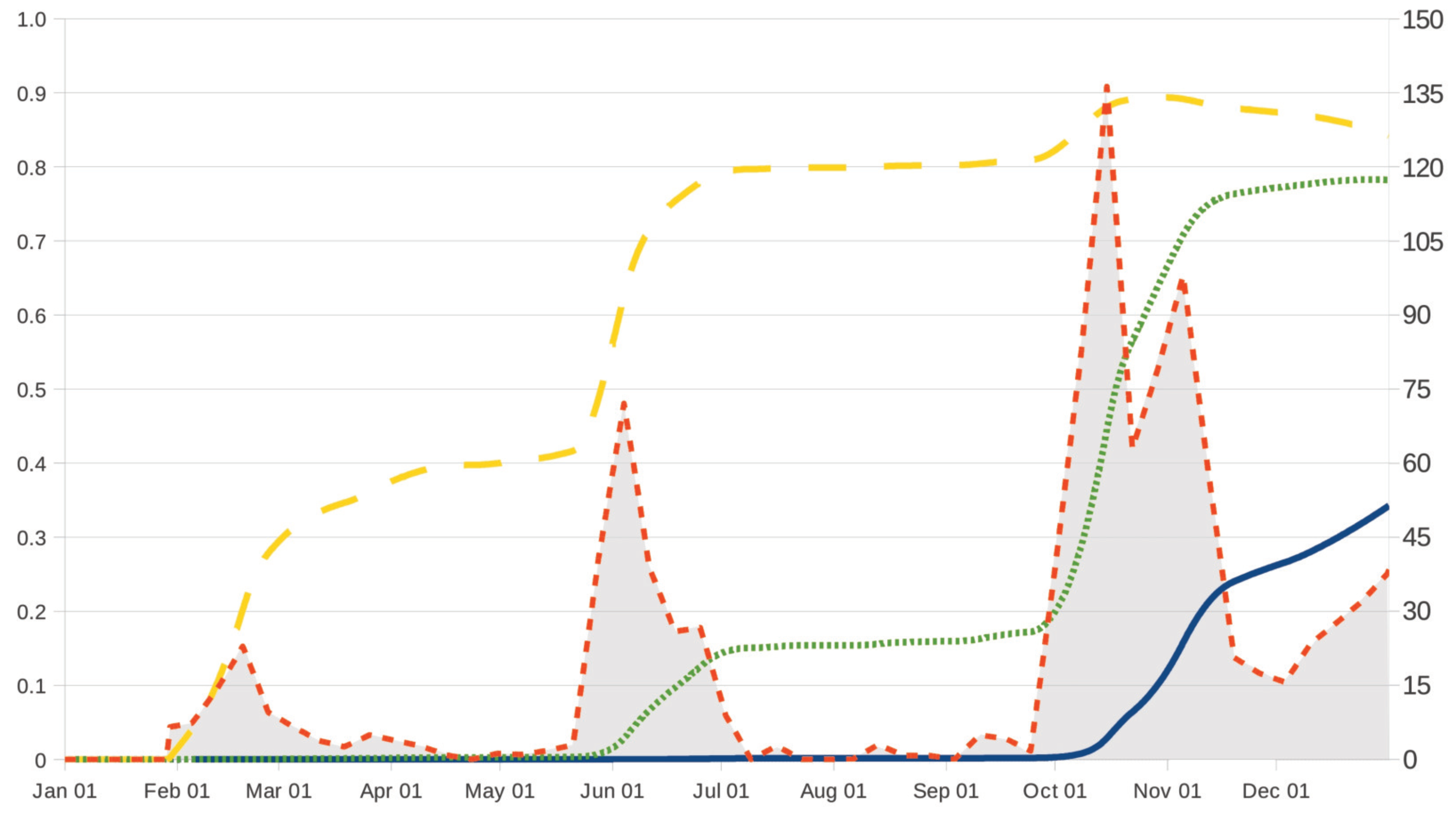
Figure A1.
The age-dependent probability as a function of the age with year, for (broken line), 4 (dotted line) and 8 (solid line), and increments in the number of infective larvae on the small intestine (shaded area, right vertical axis).
Figure A1.
The age-dependent probability as a function of the age with year, for (broken line), 4 (dotted line) and 8 (solid line), and increments in the number of infective larvae on the small intestine (shaded area, right vertical axis).

Table A2.
Intervention instants versus the index p and the lower bound for effectiveness (Criterion 1) for . Grazing strategies TS and TM with the anthelmintics ivermectin (B), fenbendazole (C) and albendazole (D).
Table A2.
Intervention instants versus the index p and the lower bound for effectiveness (Criterion 1) for . Grazing strategies TS and TM with the anthelmintics ivermectin (B), fenbendazole (C) and albendazole (D).
| p | |||||||||
|---|---|---|---|---|---|---|---|---|---|
| 0.1 | [170, 365) | 0.70 | TS | —– | —– | —– | —– | —– | —– |
| TM | [170, 278] | 170 | [170, 319] | 273 | [170, 308] | 272 | |||
| 0.60 | TS | —– | —– | [336, 339] | 336 | —– | —– | ||
| TM | [170 ,301] | 170 | [170, 344] | 273 | [170, 342] | 272 | |||
| 0.50 | TS | —– | —– | [308, 344] | 308 | [313, 343] | 313 | ||
| TM | [170, 343] | 170 | [170, 348] | 273 | [170, 346] | 272 | |||
| 0.2 | [274, 365) | 0.70 | TS | —– | —– | —– | —– | —– | —– |
| TM | [274, 278] | 274 | [274, 319] | 274 | [274, 308] | 274 | |||
| 0.60 | TS | —– | —– | [336, 339] | 336 | —– | —– | ||
| TM | [274, 301] | 274 | [274, 344] | 274 | [274, 342] | 274 | |||
| 0.50 | TS | —– | —– | [308, 344] | 308 | [313, 343] | 313 | ||
| TM | [274, 343] | 274 | [274, 348] | 274 | [274, 346] | 274 | |||
| 0.3 | [281, 365) | 0.70 | TS | —– | —– | —– | —– | —– | —– |
| TM | —– | —– | [281, 319] | 281 | [281, 308] | 281 | |||
| 0.60 | TS | —– | —– | [336, 339] | 336 | —– | —– | ||
| TM | [281, 301] | 281 | [281, 344] | 281 | [281, 342] | 281 | |||
| 0.50 | TS | —– | —– | [308, 344] | 308 | [313, 343] | 313 | ||
| TM | [281, 343] | 281 | [281, 348] | 281 | [281, 346] | 281 | |||
| 0.4 | [286, 365) | 0.70 | TS | —– | —– | —– | —– | —– | —– |
| TM | —– | —– | [286, 319] | 286 | [286, 308] | 286 | |||
| 0.60 | TS | —– | —– | [336, 339] | 336 | —– | —– | ||
| TM | [286, 301] | 286 | [286, 344] | 286 | [286, 342] | 286 | |||
| 0.50 | TS | —– | —– | [308, 344] | 308 | [313, 343] | 313 | ||
| TM | [286, 343] | 286 | [286, 348] | 286 | [286, 346] | 286 | |||
| 0.5 | [290, 365) | 0.70 | TS | —– | —– | —– | —– | —– | —– |
| TM | —– | —– | [290, 319] | 290 | [290, 308] | 290 | |||
| 0.60 | TS | —– | —– | [336, 339] | 336 | —– | —– | ||
| TM | [290, 301] | 290 | [290, 344] | 290 | [290, 342] | 290 | |||
| 0.50 | TS | —– | —– | [308, 344] | 308 | [313, 343] | 313 | ||
| TM | [290, 343] | 290 | [290, 348] | 290 | [290, 346] | 290 | |||
| 0.6 | [298, 365) | 0.70 | TS | —– | —– | —– | —– | —– | —– |
| TM | —– | —– | [298, 319] | 298 | [298, 308] | 298 | |||
| 0.60 | TS | —– | —– | [336, 339] | 336 | —– | —– | ||
| TM | [298, 301] | 298 | [298, 344] | 298 | [298, 342] | 298 | |||
| 0.50 | TS | —– | —– | [308, 344] | 308 | [313, 343] | 313 | ||
| TM | [298, 343] | 298 | [298, 348] | 298 | [298, 346] | 298 | |||
| 0.7 | [308, 365) | 0.70 | TS | —– | —– | —– | —– | —– | —– |
| TM | —– | —– | [308, 319] | 308 | [308, 308] | 308 | |||
| 0.60 | TS | —– | —– | [336, 339] | 336 | —– | —– | ||
| TM | —– | —– | [308, 344] | 308 | [308, 342] | 308 | |||
| 0.50 | TS | —– | —– | [308, 344] | 308 | [313, 343] | 313 | ||
| TM | [308, 343] | 308 | [308, 348] | 308 | [308, 346] | 308 |
Table A3.
Intervention instants versus the index p and the upper bound for the cost of intervention (Criterion 2) for . Grazing strategies TS and TM with the anthelmintics ivermectin (B), fenbendazole (C) and albendazole (D).
Table A3.
Intervention instants versus the index p and the upper bound for the cost of intervention (Criterion 2) for . Grazing strategies TS and TM with the anthelmintics ivermectin (B), fenbendazole (C) and albendazole (D).
| p | |||||||||
|---|---|---|---|---|---|---|---|---|---|
| 0.1 | [170, 365) | 0.25 | TS | [286, 363] | 358 | [268, 363] | 338 | [270, 363] | 338 |
| TM | [170, 363] | 170 | [170, 363] | 273 | [170, 363] | 272 | |||
| 0.20 | TS | [299, 362] | 358 | [279, 362] | 338 | [281, 361] | 338 | ||
| TM | [170, 362] | 170 | [170, 362] | 273 | [170, 362] | 272 | |||
| 0.15 | TS | —– | —– | [290, 346] | 338 | [292, 344] | 338 | ||
| TM | [170, 350] | 170 | [170, 350] | 273 | [170, 348] | 272 | |||
| 0.2 | [274, 365) | 0.25 | TS | [286, 363] | 358 | [274, 363] | 338 | [274, 363] | 338 |
| TM | [274, 363] | 274 | [274, 363] | 274 | [274, 363] | 274 | |||
| 0.20 | TS | [299, 362] | 358 | [279, 362] | 338 | [281, 361] | 338 | ||
| TM | [274, 362] | 274 | [274, 362] | 274 | [274, 362] | 274 | |||
| 0.15 | TS | —– | —– | [290, 346] | 338 | [292, 344] | 338 | ||
| TM | [274, 350] | 274 | [274, 350] | 274 | [274, 348] | 274 | |||
| 0.3 | [281, 365) | 0.25 | TS | [286, 363] | 358 | [281, 363] | 338 | [281, 363] | 338 |
| TM | [281, 363] | 281 | [281, 363] | 281 | [281, 363] | 281 | |||
| 0.20 | TS | [299, 362] | 358 | [281, 362] | 338 | [281, 361] | 338 | ||
| TM | [281, 362] | 281 | [281, 362] | 281 | [281, 362] | 281 | |||
| 0.15 | TS | —– | —– | [290, 346] | 338 | [292, 344] | 338 | ||
| TM | [281, 350] | 281 | [281, 350] | 281 | [281, 348] | 281 | |||
| 0.4 | [286, 365) | 0.25 | TS | [286, 363] | 358 | [286, 363] | 338 | [286, 363] | 338 |
| TM | [286, 363] | 286 | [286, 363] | 286 | [286, 363] | 286 | |||
| 0.20 | TS | [299, 362] | 358 | [286, 362] | 338 | [286, 361] | 338 | ||
| TM | [286, 362] | 286 | [286, 362] | 286 | [286, 362] | 286 | |||
| 0.15 | TS | —– | —– | [290, 346] | 338 | [292, 344] | 338 | ||
| TM | [286, 350] | 286 | [286, 350] | 286 | [286, 348] | 286 | |||
| 0.5 | [290, 365) | 0.25 | TS | [290, 363] | 358 | [290, 363] | 338 | [290, 363] | 338 |
| TM | [290, 363] | 290 | [290, 363] | 290 | [290, 363] | 290 | |||
| 0.20 | TS | [299, 362] | 358 | [290, 362] | 338 | [290, 361] | 338 | ||
| TM | [290, 362] | 290 | [290, 362] | 290 | [290, 362] | 290 | |||
| 0.15 | TS | —– | —– | [290, 346] | 338 | [292, 344] | 338 | ||
| TM | [290, 350] | 290 | [290, 350] | 290 | [290, 348] | 290 | |||
| 0.6 | [298, 365) | 0.25 | TS | [298, 363] | 358 | [298, 363] | 338 | [298, 363] | 338 |
| TM | [298, 363] | 298 | [298, 363] | 298 | [298, 363] | 298 | |||
| 0.20 | TS | [299, 362] | 358 | [298, 362] | 338 | [298, 361] | 338 | ||
| TM | [298, 362] | 298 | [298, 362] | 298 | [298, 362] | 298 | |||
| 0.15 | TS | —– | —– | [298, 346] | 338 | [298, 344] | 338 | ||
| TM | [298, 350] | 298 | [298, 350] | 298 | [298, 348] | 298 | |||
| 0.7 | [308, 365) | 0.25 | TS | [308, 363] | 358 | [308, 363] | 338 | [308, 363] | 338 |
| TM | [308, 363] | 308 | [308, 363] | 308 | [308, 363] | 308 | |||
| 0.20 | TS | [308, 362] | 358 | [308, 362] | 338 | [308, 361] | 338 | ||
| TM | [308, 362] | 308 | [308, 362] | 308 | [308, 362] | 308 | |||
| 0.15 | TS | —– | —– | [308, 346] | 338 | [308, 344] | 338 | ||
| TM | [308, 350] | 308 | [308, 350] | 308 | [308, 348] | 308 |
An examination of the resulting instants in Table A1, Table A2 and Table A3 reveals the following important consequences:
- (i)
- In applying Criterion 1 (respectively, Criterion 2) to grazing strategy TM, values of the lower bound for effectiveness (respectively, the upper bound for the cost of intervention) result in identical intervention instants , irrespective of the anthelmintic drug, with the exception of the case . More concretely, we observe that, in the case , identical intervention instants are derived for each fixed anthelmintic drug, but a replacement of the predetermined drug by another anthelmintic results in different intervention instants.
- (ii)
- For every anthelmintic drug and fixed index p, Criteria 1 and 2 applied to grazing strategy TM yield identical intervention instants , with the exception of those pairs for the anthelmintic ivermectin leading us to empty subsets . In order to maintain high values of the minimum level of effectiveness (Criterion 1), we have therefore to handle smaller values of the index p ( and in Table A2) for grazing strategy TM, which means that low-risk intervention instants should become potential intervention instants.
- (iii)
- For every anthelmintic, the intervention instant derived in grazing strategy TM behaves as an increasing function of the index p, regardless of the control criterion.
- (iv)
- For every anthelmintic and fixed value , the intervention instant in grazing strategy TS appears to be constant as a function of the index p. This is in agreement with the fact that the maximum levels of effectiveness (Figure 2) and the minimum costs of intervention (Figure 3) are observed at the end of the year (November–December), in such a way that this period of time always consists of potential intervention instants (Figure A1) for the index p ranging between and .
- (v)
- In contrast to grazing strategies TS and TM, the values for grazing strategy UM lead us to empty subsets of potential intervention instants, with the exception of the pair . This observation is closely related to the monotonic behaviour of the effectiveness (Figure 2) and cost (Figure 3) functions, which links the first months of the year to the highest effectiveness and the minimum cost of intervention.
- (vi)
- The upper limit of the set in Table A1, Table A2 and Table A3 is always at Day 365, which can be readily explained from the monotone behaviour (Figure A1) of the age-dependent probability in the case . It is clear that other thresholds will not necessarily yield Day 365; for example, in the case with .
- (vii)
- For strategies UM (Table A1) and TM (Table A2 and Table A3), the lower limits of the resulting sets and always coincide with the lower limit of the set of potential intervention instants , but this is not the case for strategy TS. This means that an early movement of the host to safe pasture should lead to feasible intervention instants.
The values of the effectiveness and the cost of intervention for instants in Table A1, Table A2 and Table A3 are listed in Table 1 and analysed in more detail in Section 3.2.
References
- Sutherland, I.; Scott, I. Gastrointestinal Nematodes of Sheep and Cattle. Biology and Control; Wiley-Blackwell: Chichester, UK, 2010. [Google Scholar]
- Taylor, M.A.; Coop, R.L.; Wall, R.L. Veterinary Parasitology, 3rd ed.; Blackwell: Oxford, UK, 2007. [Google Scholar]
- Bjørn, H.; Monrad, J.; Nansen, P. Anthelmintic resistance in nematode parasites of sheep in Denmark with special emphasis on levamisole resistance in Ostertagia circumcincta. Acta Vet. Scand. 1991, 32, 145–154. [Google Scholar] [PubMed]
- Entrocasso, C.; Alvarez, L.; Manazza, J.; Lifschitz, A.; Borda, B.; Virkel, G.; Mottier, L.; Lanusse, C. Clinical efficacy assessment of the albendazole-ivermectin combination in lambs parasited with resistant nematodes. Vet. Parasitol. 2008, 155, 249–256. [Google Scholar] [CrossRef] [PubMed]
- Stear, M.J.; Doligalska, M.; Donskow-Schmelter, K. Alternatives to anthelmintics for the control of nematodes in livestock. Parasitology 2007, 134, 139–151. [Google Scholar] [CrossRef] [PubMed]
- Hein, W.R.; Shoemaker, C.B.; Heath, A.C.G. Future technologies for control of nematodes of sheep. N. Z. Vet. J. 2001, 49, 247–251. [Google Scholar] [CrossRef] [PubMed]
- Knox, D.P. Technological advances and genomics in metazoan parasites. Int. J. Parasitol. 2004, 34, 139–152. [Google Scholar] [CrossRef] [PubMed]
- Sayers, G.; Sweeney, T. Gastrointestinal nematode infection in sheep—A review of the alternatives to anthelmintics in parasite control. Anim. Health Res. Rev. 2005, 6, 159–171. [Google Scholar] [CrossRef] [PubMed]
- Waller, P.J.; Thamsborg, S.M. Nematode control in ‘green’ ruminant production systems. Trends Parasitol. 2004, 20, 493–497. [Google Scholar] [CrossRef] [PubMed] [Green Version]
- Smith, G.; Grenfell, B.T.; Isham, V.; Cornell, S. Anthelmintic resistance revisited: Under-dosing, chemoprophylactic strategies, and mating probabilities. Int. J. Parasitol. 1999, 29, 77–91. [Google Scholar] [CrossRef]
- Praslička, J.; Bjørn, H.; Várady, M.; Nansen, P.; Hennessy, D.R.; Talvik, H. An in vivo dose-response study of fenbendazole against Oesophagostomum dentatum and Oesophagostomum quadrispinulatum in pigs. Int. J. Parasitol. 1997, 27, 403–409. [Google Scholar] [CrossRef]
- Coles, G.C.; Roush, R.T. Slowing the spread of anthelmintic resistant nematodes of sheep and goats in the United Kingdom. Vet. Res. 1992, 130, 505–510. [Google Scholar] [CrossRef]
- Prichard, R.K.; Hall, C.A.; Kelly, J.D.; Martin, I.C.A.; Donald, A.D. The problem of anthelmintic resistance in nematodes. Aust. Vet. J. 1980, 56, 239–250. [Google Scholar] [CrossRef] [PubMed]
- Anderson, R.M.; May, R.M. Infectious Diseases of Humans: Dynamics and Control; Oxford University Press: Oxford, UK, 1992. [Google Scholar]
- Marion, G.; Renshaw, E.; Gibson, G. Stochastic effects in a model of nematode infection in ruminants. IMA J. Math. Appl. Med. Biol. 1998, 15, 97–116. [Google Scholar] [CrossRef] [PubMed]
- Cornell, S.J.; Isham, V.S.; Grenfell, B.T. Stochastic and spatial dynamics of nematode parasites in farmed ruminants. Proc. R. Soc. B Biol. Sci. 2004, 271, 1243–1250. [Google Scholar] [CrossRef] [PubMed] [Green Version]
- Roberts, M.G.; Grenfell, B.T. The population dynamics of nematode infections of ruminants: Periodic perturbations as a model for management. IMA J. Math. Appl. Med. Biol. 1991, 8, 83–93. [Google Scholar] [CrossRef] [PubMed]
- Roberts, M.G.; Grenfell, B.T. The population dynamics of nematode infections of ruminants: The effect of seasonality in the free-living stages. IMA J. Math. Appl. Med. Biol. 1992, 9, 29–41. [Google Scholar] [CrossRef] [PubMed]
- Allen, L.J.S. An Introduction to Stochastic Processes with Applications to Biology; Pearson Education: Hoboken, NJ, USA, 2003. [Google Scholar]
- Gómez-Corral, A.; López García, M. Control strategies for a stochastic model of host-parasite interaction in a seasonal environment. J. Theor. Biol. 2014, 354, 1–11. [Google Scholar] [CrossRef] [PubMed]
- Abbott, K.A.; Taylor, M.; Stubbings, L.A. Sustainable Worm Control Strategies for Sheep, 4th ed.; A Technical Manual for Veterinary Surgeons and Advisers; SCOPS: Worcestershire, UK, 2012; Available online: http://www.scops.org.uk/workspace/pdfs/scops-technical-manual-4th-edition-updated-september-2013.pdf (accessed on 1 June 2018).
- Uriarte, J.; Llorente, M.M.; Valderrábano, J. Seasonal changes of gastrointestinal nematode burden in sheep under an intensive grazing system. Vet. Parasitol. 2003, 118, 79–92. [Google Scholar] [CrossRef] [PubMed]
- Faragó, I.; Havasi, A.; Horváth, R. On the order of operator splitting methods for time-dependent linear systems of differential equations. Int. J. Numer. Anal. Model. Ser. B 2011, 2, 142–154. [Google Scholar]
- Nasreen, S.; Jeelani, G.; Sheikh, F.D. Efficacy of different anthelmintics against gastro-intestinal nematodes of sheep in Kashmir Valley. VetScan 2007, 2, 1. [Google Scholar]
- Kassai, T. Veterinary Helminthology; Butterworth-Heinemann: Oxford, UK, 1999. [Google Scholar]
- Barger, I.A. Genetic resistance of hosts and its influence on epidemiology. Vet. Parasitol. 1989, 32, 21–35. [Google Scholar] [CrossRef]
- Barger, I.A.; Le Jambre, L.F.; Georgi, J.R.; Davies, H.I. Regulation of Haemonchus contortus populations in sheep exposed to continuous infection. Int. J. Parasitol. 1985, 15, 529–533. [Google Scholar] [CrossRef]
- Dobson, R.J.; Waller, P.J.; Donald, A.D. Population dynamics of Trichostrongylus colubriformis in sheep: The effect of infection rate on the establishment of infective larvae and parasite fecundity. Int. J. Parasitol. 1990, 20, 347–352. [Google Scholar] [CrossRef]
- Bailey, J.N.; Kahn, L.P.; Walkden-Brown, S.W. Availability of gastro-intestinal nematode larvae to sheep following winter contamination of pasture with six nematode species on the Northern Tablelands of New South Wales. Vet. Parasitol. 2009, 160, 89–99. [Google Scholar] [CrossRef] [PubMed]
- Valderrábano, J.; Delfa, R.; Uriarte, J. Effect of level of feed intake on the development of gastrointestinal parasitism in growing lambs. Vet. Parasitol. 2002, 104, 327–338. [Google Scholar] [CrossRef]
- Grennan, E.J. Lamb Growth Rate on Pasture: Effect of Grazing Management, Sward Type and Supplementation; Teagasc Research Centre: Athenry, Ireland, 1999. [Google Scholar]
Figure 1.
State space and transitions at post-intervention instants . Grazing strategies TS and TM.

Figure 2.
Effectiveness as a function of the intervention age for year and increments in the number of infective larvae in the small intestine (shaded area, right vertical axis). Scenario US, and grazing strategies UM, TS and TM with the anthelmintics ivermectin, fenbendazole and albendazole (from top to bottom).

Figure 3.
Cost of intervention as a function of the intervention age for year and increments in the number of infective larvae in the small intestine (shaded area, right vertical axis). Scenario US, and grazing strategies UM, TS and TM with the anthelmintics ivermectin, fenbendazole and albendazole (from top to bottom).

Figure 4.
Expected proportions (top) and (bottom) versus the intervention age for year and increments in the number of infective larvae in the small intestine (shaded area, right vertical axis). Scenario US, and grazing strategies UM, TS and TM with the anthelmintic fenbendazole.
Figure 4.
Expected proportions (top) and (bottom) versus the intervention age for year and increments in the number of infective larvae in the small intestine (shaded area, right vertical axis). Scenario US, and grazing strategies UM, TS and TM with the anthelmintic fenbendazole.

Figure 5.
The mass function of the parasite burden at age year. Scenario US and grazing strategies UM, TS and TM (from left to right) with the anthelmintic ivermectin as the intervention prescribed at age .
Figure 5.
The mass function of the parasite burden at age year. Scenario US and grazing strategies UM, TS and TM (from left to right) with the anthelmintic ivermectin as the intervention prescribed at age .

Figure 6.
The mass function of the parasite burden at age year. Scenario US and grazing strategy TM with the anthelmintics ivermectin, fenbendazole and albendazole (from left to right) as the intervention prescribed at ages , 273 and 272, respectively.
Figure 6.
The mass function of the parasite burden at age year. Scenario US and grazing strategy TM with the anthelmintics ivermectin, fenbendazole and albendazole (from left to right) as the intervention prescribed at ages , 273 and 272, respectively.

Table 1.
Effectiveness and cost of intervention. Scenario US and grazing strategies UM, TS and TM with the anthelmintics ivermectin, fenbendazole and albendazole.
Table 1.
Effectiveness and cost of intervention. Scenario US and grazing strategies UM, TS and TM with the anthelmintics ivermectin, fenbendazole and albendazole.
| Strategy (s) | Anthelmintic | Criteria | |||||
|---|---|---|---|---|---|---|---|
| US | — | — | — | 0.06072 | 0.49951 | 0.68645 | 0.14746 |
| UM | 170 | 1 & 2 | 0.54431 | 0.11049 | 0.79996 | 0.09726 | |
| 274 | 2 | 0.45540 | 0.12524 | 0.76629 | 0.09983 | ||
| 281 | 2 | 0.38981 | 0.14216 | 0.74973 | 0.10267 | ||
| 286 | 2 | 0.32115 | 0.16811 | 0.73306 | 0.10715 | ||
| 290 | 2 | 0.26634 | 0.19763 | 0.72023 | 0.11233 | ||
| 298 | 2 | 0.20886 | 0.24130 | 0.70769 | 0.11984 | ||
| TS | ivermectin | 358 | 2 | 0.41766 | 0.16608 | 0.69160 | 0.14217 |
| fenbendazole | 308 | 1 | 0.50340 | 0.12350 | 0.75871 | 0.10433 | |
| 336 | 1 | 0.60161 | 0.13144 | 0.71941 | 0.12421 | ||
| 338 | 2 | 0.60604 | 0.13209 | 0.71613 | 0.12578 | ||
| albendazole | 313 | 1 | 0.50240 | 0.12842 | 0.74908 | 0.10793 | |
| 338 | 2 | 0.57385 | 0.13407 | 0.71312 | 0.12626 | ||
| TM | ivermectin | 170 | 1 & 2 | 0.73224 | 0.09721 | 0.86987 | 0.09525 |
| 274 | 1 & 2 | 0.71025 | 0.09797 | 0.82480 | 0.09580 | ||
| 281 | 1 & 2 | 0.69119 | 0.09877 | 0.81634 | 0.09602 | ||
| 286 | 1 & 2 | 0.66653 | 0.10011 | 0.80686 | 0.09644 | ||
| 290 | 1 & 2 | 0.64110 | 0.10197 | 0.79743 | 0.09713 | ||
| 298 | 1 & 2 | 0.61142 | 0.10528 | 0.78209 | 0.09911 | ||
| 308 | 1 & 2 | 0.56977 | 0.11374 | 0.76202 | 0.10372 | ||
| fenbendazole | 273 | 1 & 2 | 0.79086 | 0.09589 | 0.83891 | 0.09557 | |
| 274 | 1 & 2 | 0.79080 | 0.09589 | 0.83820 | 0.09558 | ||
| 281 | 1 & 2 | 0.78559 | 0.09601 | 0.83107 | 0.09573 | ||
| 286 | 1 & 2 | 0.77604 | 0.09636 | 0.82304 | 0.09605 | ||
| 290 | 1 & 2 | 0.76467 | 0.09707 | 0.81476 | 0.09662 | ||
| 298 | 1 & 2 | 0.75182 | 0.09895 | 0.79922 | 0.09852 | ||
| 308 | 1 & 2 | 0.72721 | 0.10573 | 0.77734 | 0.10310 | ||
| albendazole | 272 | 1 & 2 | 0.78128 | 0.09605 | 0.83749 | 0.09558 | |
| 274 | 1 & 2 | 0.78102 | 0.09606 | 0.83605 | 0.09560 | ||
| 281 | 1 & 2 | 0.77361 | 0.09623 | 0.82838 | 0.09576 | ||
| 286 | 1 & 2 | 0.76132 | 0.09666 | 0.81971 | 0.09610 | ||
| 290 | 1 & 2 | 0.74737 | 0.09747 | 0.81089 | 0.09671 | ||
| 298 | 1 & 2 | 0.73134 | 0.09945 | 0.79492 | 0.09867 | ||
| 308 | 1 & 2 | 0.70211 | 0.10641 | 0.77271 | 0.10336 |
Table 2.
Indexes reduction in the mean infection level (RMIL) and reduction in the total lost probability (RTLP) for strategies UM, TS and TM with the anthelmintic fenbendazole.
Table 2.
Indexes reduction in the mean infection level (RMIL) and reduction in the total lost probability (RTLP) for strategies UM, TS and TM with the anthelmintic fenbendazole.
| Strategy (s) | Criteria | |||
|---|---|---|---|---|
| UM | 170 | |||
| 2 | 274 | |||
| 2 | 281 | |||
| 2 | 286 | |||
| 2 | 290 | |||
| 2 | 298 | |||
| Midsummer | 195 | |||
| TS | 1 | 308 | ||
| 1 | 336 | |||
| 2 | 338 | |||
| Maximum pasture contamination | 287 | |||
| TM | 273 | |||
| 274 | ||||
| 281 | ||||
| 286 | ||||
| 290 | ||||
| 298 | ||||
| 308 | ||||
| Midsummer | 195 |
© 2018 by the authors. Licensee MDPI, Basel, Switzerland. This article is an open access article distributed under the terms and conditions of the Creative Commons Attribution (CC BY) license (http://creativecommons.org/licenses/by/4.0/).
Share and Cite
MDPI and ACS Style
Gómez-Corral, A.; López-García, M. A Within-Host Stochastic Model for Nematode Infection. Mathematics 2018, 6, 143. https://doi.org/10.3390/math6090143
AMA Style
Gómez-Corral A, López-García M. A Within-Host Stochastic Model for Nematode Infection. Mathematics. 2018; 6(9):143. https://doi.org/10.3390/math6090143
Chicago/Turabian StyleGómez-Corral, Antonio, and Martín López-García. 2018. "A Within-Host Stochastic Model for Nematode Infection" Mathematics 6, no. 9: 143. https://doi.org/10.3390/math6090143
Note that from the first issue of 2016, this journal uses article numbers instead of page numbers. See further details here.