
Sentiment Difficulty in Aspect-Based Sentiment Analysis

Aix-Marseille Université, Université de Toulon, CNRS, LIS, 13007 Marseille, France
*
Author to whom correspondence should be addressed.
Mathematics 2023, 11(22), 4647; https://doi.org/10.3390/math11224647
Submission received: 14 October 2023
/
Revised: 9 November 2023
/
Accepted: 10 November 2023
/
Published: 14 November 2023
(This article belongs to the Special Issue Current Trends in Natural Language Processing (NLP) and Human Language Technology (HLT))
Abstract
:Subjectivity is a key aspect of natural language understanding, especially in the context of user-generated text and conversational systems based on large language models. Natural language sentences often contain subjective elements, such as opinions and emotions, that make them more nuanced and complex. The level of detail at which the study of the text is performed determines the possible applications of sentiment analysis. The analysis can be done at the document or paragraph level, or, even more granularly, at the aspect level. Many researchers have studied this topic extensively. The field of aspect-based sentiment analysis has numerous data sets and models. In this work, we initiate the discussion around the definition of sentence difficulty in this context of aspect-based sentiment analysis. To assess and quantify the difficulty of the aspect-based sentiment analysis, we conduct an experiment using three data sets: “Laptops”, “Restaurants”, and “MTSC” (Multi-Target-dependent Sentiment Classification), along with 21 learning models from scikit-learn. We also use two textual representations, TF-IDF (Terms frequency-inverse document frequency) and BERT (Bidirectional Encoder Representations from Transformers), to analyze the difficulty faced by these models in performing aspect-based sentiment analysis. Additionally, we compare the models with a fine-tuned version of BERT on the three data sets. We identify the most challenging sentences using a combination of classifiers in order to better understand them. We propose two strategies for defining sentence difficulty. The first strategy is binary and considers sentences as difficult when the classifiers are unable to correctly assign the sentiment polarity. The second strategy uses a six-level difficulty scale based on how many of the top five best-performing classifiers can correctly identify sentiment polarity. These sentences with assigned difficulty classes are then used to create predictive models for early difficulty detection. The purpose of estimating the difficulty of aspect-based sentiment analysis is to enhance performance while minimizing resource usage.
Keywords:
sentiment analysis; aspect-based sentiment analysis; difficulty; sentiment polarity; text representationMSC:
68T50; 68T071. Introduction
Sentiment analysis, also known as opinion mining, is a field of natural language processing that aims to automatically identify and extract subjective information from texts. Sentiment analysis has numerous applications, ranging from marketing to politics, and it has become an increasingly popular topic of research in the past decade [1,2]. Sentiment analysis can be used to identify the sentiments of customers towards a particular product, the opinions of voters towards a political candidate, or the emotions of patients towards their medical condition, among other applications.
Despite recent advancements in sentiment analysis, the detection and analysis of sentiments remain challenging due to several factors. One of the most significant challenges in sentiment analysis is the ambiguity of language [3,4,5]. For example, the word “hot” can refer to temperature, attractiveness, or anger, and it may be difficult for algorithms to determine which meaning is intended in a particular text. In the sentence “This new restaurant has some hot dishes”, the sentiment may be positive because the dishes are delicious or negative because they are too spicy. Ambiguity in language is further complicated by the use of slang, idioms, and regional dialects, which can vary widely even within the same language. For instance, the phrase “cool beans” means “excellent” in American English, but it may be meaningless or confusing to non-native speakers.
Another challenge in sentiment analysis is the detection of tone and sarcasm [6,7,8]. Texts often contain tones that can be difficult for algorithms to detect, and sarcasm can be especially challenging. For example, a person might say “great” in a sarcastic tone to indicate the opposite of what the word usually means. In the sentence “I love spending hours in traffic every day”, the sentiment may be negative despite the positive connotation of the word “love” because the text is sarcastic. Detecting the tone of a text is crucial in understanding the sentiment, as the same words can have different meanings depending on the tone in which they are expressed.
Cultural and contextual differences also pose a challenge to sentiment analysis [9]. Sentiments can vary based on culture and context, and what might be considered positive in one culture may not be the same in another. For example, in some cultures, being direct and blunt is considered a positive trait, while in others, it may be seen as negative. Let us analyze the sentence “The government imposed a strict lockdown to prevent the spread of COVID-19”. This sentence expresses a positive sentiment towards the aspect of lockdown, as it implies that the government is taking proactive measures to protect the public health and safety. However, this sentiment may not be shared by people from cultures that value individual freedom and autonomy more than collective welfare and security. For them, the lockdown may be seen as a negative aspect that infringes on their personal rights and choices. Sentiment analysis algorithms must be trained on diverse data sets to overcome such differences.
Data quality and quantity are also crucial factors in the effectiveness of sentiment analysis algorithms. Sentiment analysis algorithms require large amounts of high-quality data to train effectively. However, it can be challenging to gather such data, especially for less common languages or topics. Additionally, data quality issues such as noise, missing data, or bias [10] can affect the accuracy of sentiment analysis. In the sentence “I bought a phone from XYZ company, and it’s terrible”, the sentiment may be negative towards the phone, but it could also be negative towards the company or the customer service. Without additional context or information, it may be difficult for algorithms to determine the sentiment accurately.
One way to perform sentiment analysis is to examine different levels of granularity: the whole document, a single paragraph, a sentence, or even a specific aspect. However, each level of analysis may encounter the challenges that are discussed previously in this introduction. In this work, we will focus on the most fine-grained level, the aspect level. Indeed, apsect-based is the level for which research is currently the most productive, and consequently also generates the production of corpora whose expressiveness of sentiment is more subtle and therefore potentially more difficult to analyze.
Finally, sentiment analysis algorithms may exhibit bias [10] and subjectivity due to the training data used or the biases of the developers. For example, if a sentiment analysis algorithm was trained on texts from a particular political perspective, it may not perform well on texts from other perspectives. Bias and subjectivity can also arise from the choice of sentiment lexicons, which are dictionaries of words and phrases that are labeled.
Recent years have seen advances in language models, particularly the emergence of BERT [11] and GPT [12]. These have enabled algorithms to better capture the semantics of texts, resulting in a marked improvement in performance. This raises the question of whether the challenges mentioned above still exist, and if so, how algorithms manage to overcome them. In this article, we explore how algorithms handle these difficulties and which subjective sentences pose the greatest challenge.
Contrary to the usual focus in current aspect-based sentiment analysis research, our aim does not involve achieving better results or introducing a new classification model. Rather, it is to comprehend why existing models are not working in some cases and why some data sets are “simpler” than others. The aim is therefore to observe the behavior of classification models in the aspect-based sentiment analysis task and to estimate the degree of difficulty of the analyzed sentences. Thus, estimating the difficulty of sentiment analysis could enhance performance while minimizing resource usage.
In order to better understand the aspect-based sentiment analysis difficulty, we raise the following research questions:
- RQ1: How to define difficulty in aspect-based sentiment analysis?
- RQ2: Is difficulty data set-dependent?
- RQ3: What is the impact of text representation on performance?
- RQ4: What is the impact of classification models on performance?
- RQ5: Are we able to predict difficulty?
- RQ6: How to better understand difficult sentences (qualitative analysis on difficult sentences)?
To summarize, in order to answer these six research questions, we propose in our work to:
- Select 3 data sets whose purpose is to perform aspect-based classification. The data sets have been created at a 6–7 year time distance, and choosing three data sets that span over such a large period of time would reflect the evolution of the field;
- Select 21 models and two different text representations in order to analyze their respective behavior and performance when faced with aspect-based sentiment analysis;
- Conduct numerous experiments in order to better understand the challenges faced by the models;
- Investigate automatic sentence difficulty definition and estimation using learning-based models.
The remainder of this paper is organized as follows. Section 2 provides an overview of aspect-based sentiment analysis, text representation models and the concept of difficulty in Information Retrieval. Section 3 presents three different data sets used in the experiments. Then, Section 4 presents the 2 text representations that have been used and Section 5 presents the different used models and the employed implementations. Section 6 explains the experimental protocol and presents the aspect-based sentiment polarity classification results. Section 7 proposes difficulty definitions and tests if the difficulty may be predicted, while Section 8 discusses the results and answers the research questions. Finally, Section 9 concludes the paper and suggests directions for future work.
2. Related Work
We further divide our related work into themes that influence our analysis, including Sentiment Analysis, Aspect-based Sentiment Analysis, Text Representation, and Query Difficulty in Information Retrieval.
2.1. Sentiment Analysis and Aspect-Based Sentiment Analysis
The goal of sentiment analysis is to identify and categorize emotions and sentiments expressed in written text automatically. Sentiment analysis is a fairly broad area of research and can be defined at several levels—at a document level, paragraph level, or sentence level—but also at a much finer level, at an aspect level, which is the element on which subjectivity is focused. In the literature research works are often classified into three categories: machine learning, deeplearning, and ensemble learning. Among the most effective machine learning techniques for this task are naive Bayes [13,14,15] and SVM [16,17,18]. Algorithms based on deeplearning [19] include RNNs [20,21], LSTMs [22,23,24], and transformers [25,26]. Ensemble-based methods [27] combine multiple classifiers, which can fall into either of the previous categories. In response to the large amount of work on the subject of sentiment analysis, a number of surveys have been carried out recently [27,28,29,30]. However, for several years now, research has been more focused on multimodal, multilingual sentiment analysis and on the finest level of sentiment analysis: the aspect-based level.
The finesse of the analysis at the aspect level means that in the vast majority of cases we can be sure of having a uniqueness of subjectivity. In other words, there are not two opposite degrees of subjectivity for the same aspect. This aspect of sentiment analysis is often divided into two distinct tasks; the first consists of finding and extracting the aspects. The second is to estimate the subjectivity, generally reducing the problem of estimating the degree of subjectivity to a simpler problem of classification. This involves classifying the sentences or nominal phrases containing the aspects as neutral (no subjectivity), positive (the author speaks positively about the aspect), and negative (the author speaks negatively about the aspect). Sometimes the scale of values used is broader (often 5 classes) and sometimes there are other classes, as is the case for the data we are going to use (e.g., conflict). In this document, we will only deal with the second task, i.e., the classification of subjectivity by taking aspects into account. To carry out this task, the methods and models used are relatively similar to those used in sentiment analysis at a coarser level. This research was introduced by the seminal work of [31] and has been developed with the production of numerous models and data sets in various languages. As in the more general context of sentiment analysis, we found similar algorithms but adapted them to the task. Among these algorithms, we can cite the use of SVMs [32] and Naïve Bayes [33]. More recently, the advent of deeplearning has considerably improved model performance. For example, there are models using RNNs, LSTMs [34,35,36], and transformers [37,38]. For further reading, one can also refer to surveys on the subject [39,40,41]. As the most recent work has focused on aspect-based analysis, the recent corpora produced for this task seem to us to have a more subtle expressivity of sentiment. This is why, in order to have a more thorough study of the difficulty in sentiment analysis, we have focused in this work on the aspect-based sentiment analysis, although the conclusions and models we obtain can be applied to sentiment analysis in a general way.
2.2. Text Representation
Text representation for machine learning models has always been a major issue. Initially, the vector representation of documents was only done by taking into account the presence or absence of terms in the document. This representation was then improved by taking into account the frequency of terms in the documents and in the collection [42]. However, such representations take no account of the semantics expressed in the sentences. With the arrival of deeplearning and the emergence of less sparse representations, semantic aspects have been better taken into account. These representations were democratized thanks to the work of [43] and then improved through the work of [44]. The emergence of transformers has also made it possible to obtain new, more efficient representations [11].
2.3. Difficulty in Information Retrieval
As we have already noted, the various existing challenges in aspect-based sentiment analysis make it difficult to classify sentences. Therefore, it is important to detect such difficult sentences to choose a different strategy in order to extract the expressed sentiment. Having multiple strategies in order to classify sentiment based on the detected difficulty helps to reduce the use of resource-intensive algorithms. Thus, we reduce the economic and ecological costs of the models. Difficulty detection is a key area of research, especially in information retrieval. In the 2000s, research on query difficulty began and many predictors were defined based on distribution [45], ambiguity [46], and complexity [47]. In the field of information retrieval, models predicting difficulty are divided according to whether they use pre- or post-retrieval predictors. Models using pre-retrieval predictors include those presented in [48,49,50]. These models use statistics on the occurrence of query terms. Among the models using post-retrieval predictors we find the work of [51,52,53,54,55]. These models will use the results of the information retrieval models to make their predictions. With the advent of deep neural networks, recent work has used such models to predict difficulty. These studies notably include [55,56]. Recently, [57,58] have raised the question of the effectiveness of evaluating the difficulty of Neural Information Retrieval based on PLM (Pre-trained Language Models).
Predicting the difficulty of a sentence in sentiment classification can not only improve the performance of the algorithms by selecting models according to the difficulty encountered, but can also make the systems more resource-efficient.
The notion of difficulty in aspect-based sentiment analysis has not yet been studied. Inspired by the work that has been conducted on information retrieval, particularly inspired by works on post-retrieval predictors, we are conducting experiments that will enable us to gain a better understanding of the notion of difficulty in this specific case. In addition, we have also sought to automate the estimation of difficulty for aspect-based sentiment analysis. In the remaining part of this paper we present the experiments that have been carried out in order to better understand where the difficulties lie in the sentiment classification task based on aspects.
3. Reference Data Sets Used for Corpus Building
In this section, we will introduce the reference data sets. These data sets have been essential because they provided the data for our corpus. Following that, we will explain the process of building the corpus. After that, we will move on to an exploratory analysis.
We used three data sets for our experiments: “Laptops”, “Restaurants”, and “MTSC”. We provide details on the data sets below. In order to perceive the temporal evolution of the difficulty of the task, we selected three corpora, each spaced about 6–7 years apart. We also chose two different objects of study: reviews and political news. The first and second corpora concern Laptop and restaurant reviews, respectively. They were published in 2009 and 2014. The third concerns political news and was published in 2021.
On each of these corpora and two different representations (TF-IDF and BERT), we carried out experiments with 21 learning models in order to discover on which corpus the models had the most difficulty. We consider a model to have difficulty if its performance is below the median of model performance for a given corpus. We also consider difficulty at a more micro level, by looking at the sentences and paragraphs posing the most difficulty for the selected models.
3.1. Laptops
The SemEval Laptop Reviews data set [59] is often associated with the laptops data set for aspect-based sentiment analysis. It was first used in the SemEval-2014 Task 4: Aspect-Based Sentiment Analysis challenge. This data set is used for two subtasks: aspect identification (Subtask 1) and aspect-oriented sentiment polarity classification (Subtask 2).
It contains more than 3000 English sentences from customer reviews of laptops. It focuses on analyzing sentiments at a more granular level, targeting various aspects or attributes of laptops such as performance, battery life, design, and usability. Expert human annotators have labeled the aspect terms of the sentences and their sentiment. A part of this data set was kept as test data by the organizers of the SemEval-2014 competition.
This data set enables researchers to analyze sentiment polarities towards specific aspects of laptops. It provides insights into customers’ preferences and satisfaction levels.
Each review may contain one or multiple aspects. Each aspect is assigned one of four possible labels: “positive”, “negative”, “neutral”, or “conflict”.
3.2. Restaurants
The restaurant data set for aspect-based sentiment analysis consists of more than 3000 English sentences from restaurant reviews initially proposed by Ganu et al. [60]. As it has already been pointed out, aspect-based sentiment analysis is different from traditional sentiment analysis which focuses on overall sentiment of reviews. The original data set includes annotations for coarse aspect categories and overall sentence polarities. It has been modified for SemEval-2014 [59] to include annotations for aspect terms occurring in the sentences (Subtask 1), aspect term polarities (Subtask 2), and aspect category-specific polarities (Subtask 4). Some errors in the original data set have been corrected. Human annotators identified the aspect terms of the sentences and their polarities (Subtasks 1 and 2). Additional restaurant reviews, not present in the original data set, have been annotated in the same manner and kept by the organisers of SemEval-2014 as test data.
This data set covers reviews related to various aspects of restaurants such as food quality, service, ambiance, price, and cleanliness. Each review is labeled with sentiment ratings for each aspect. The polarities that may be identified are “positive”, “negative”, “neutral”, and “conflict”.
3.3. MSTC
NewsMTSC is an aspect-based sentiment analysis data set proposed by the authors of [61]. It focuses on news articles about policy issues and contains over 11,000 labeled sentences sampled from online US news outlets.
Most of the sentences contain several aspects that are mentioned in the data set. The conflict class does not exist, so only three polarity levels may be encountered: “positive”, “negative”, and “neutral”.
Next, we will describe how our corpus was constructed.
3.4. Corpus Preparation
There are several files formats across the considered data sets and each data set contains multiple files. The number of attributes per data set may also vary. We have unified the data into one file per corpus, in csv format.
We have kept one id generated by us, the id from the original data set (for tracing purposes), the sentences, the start position of the aspect, the end position of the aspect, the aspect, and the polarity class. We will make the data sets publicly available upon acceptance.
For the “Laptops” corpus, there are several files in the original data set. These files come in both csv and xml formats. We excluded the files Laptops_Test_Data_PhaseA and Laptops_Test_Data_PhaseB as they do not contain annotations. We used the annotated sentences from Laptop_Train_v2 as training data and the annotated sentences from laptops-trial as test data. We merged all the data into one file named laptops.csv. It has 2407 rows in total.
The “Restaurants” corpus has the same structure as the Laptops corpus. We selected the same corresponding elements, which resulted in our restaurants.csv file with 3789 rows.
The MTSC data from the NewsMTSC corpus is in json format. The files containing the data are train, devtest_mt, and devtest_rw. We did not consider devtest_mt since it is designed to evaluate a model’s classification performance only on sentences with at least two target mentions, which is out of the scope of our research. Thus, we used train as the train data and devtest_rw (w stands for “real-world”) as the test data. The resulting data file, called MTSC.csv, contains 9885 rows in total.
This last data set contains polarity scores that we have encoded as classes. There are three possible scores: 2.0 = “negative”, 4.0 = “neutral”, and 6.0 = “positive”. We have converted the scores to their corresponding strings. The “conflict” class is not present in this corpus. Sentences with multiple aspects have been duplicated the same number of times as the number of aspects. For example, a sentence with three aspects will appear three times in the data set, one time for each aspect.
The statistics of the data sets used for the experiments are shown in Table 1.
In the following, we present our exploratory analysis conducted on the three data sets.
3.5. Exploratory Analysis
We analyzed the three data sets briefly to gain insight into their structure, detect any biases, and form hypotheses.
We first examined the polarity ratios in each data set. Figure 1 shows these ratios. The most balanced data set is “MTSC”, with of the data belonging to the negative class. The other two data sets are more unbalanced, with “Restaurants” being the most unbalanced, having of the data in the positive class and only in the conflict class. The conflict class is the rarest across all three data sets, with in “Laptops” and none in “MTSC”.
First, we look at the polarity distributions for each data set, taking into account the train/test splits.
Figure 2 shows the class occurrences in the “Laptops” data set with respect to the train and test splits. Notably, the conflict class has no occurrences in the test set. Additionally, the data set relatively maintains the positive/negative/neutral ratios in the train set (, , ) as compared to the test set (, , ).
Figure 3 illustrates the “Restaurants” data set class occurrences. The remarks for “Laptops” are concurrent with this data set as well, and we underline once more that the positive class is significantly more represented than the others.
Figure 4 shows the class occurrences for the “MTSC” data set. This data set is balanced in both the train and test splits. The conflict class does not appear in this data set.
We have decided to keep the conflict class, even though it is not found in all data sets and there is no occurrence of it in any test data. This is to preserve the original data distributions for each data set as much as possible.
We now focus on analyzing the tokens and sentences from the data sets. The results are summarized in Table 2. It is common to find duplicate sentences in the data set, as one sentence may contain multiple aspects and thus may appear more than once, by design. However, the number of unique aspects is even lower than the number of unique sentences, meaning there may be multiple sentences for one aspect. Additionally, the maximum number of tokens per aspect ranges from 6 to 31 on the Laptops and MTSC data sets, respectively. This indicates that aspects may be lengthy and not necessarily composed of only one or two words.
Following this interesting observation, we continued analyzing the number of tokens from the aspects. Figure 5a depicts the frequency of the aspects by their length in terms of the number of tokens. One may notice that the vast majority of the tokens have one or two aspects. This holds for the three data sets. There is a long-tail distribution starting from aspects with four tokens per aspect and going up to 31 tokens per aspect in the case of MTSC. The maximum number of aspects for the Restaurants data set is 19. This long-tail distribution is illustrated in Figure 5b.
To gain a better understanding of the data sets, we conducted a linguistic analysis of sentiment polarity for each data set. We calculated the average number of tokens, nouns, verbs, named entities, and adjectives per instance. The results are shown in Table 3. One may notice that the sentences from MTSC are usually longer than the sentences from the other data set. However, it has been proven for query difficulty prediction that the query length is not correlated with the Average Precision performance measure [62]. Another interesting observation is that the average number of named entities in the MTSC corpus is significantly higher than for the other two data sets. This may add up to the difficulty of aspect-based polarity classification.
We wanted to investigate if the amount of nouns, verbs, or adjectives differs depending on the sentiment class. The statistics show that the positive classes have fewer nouns and verbs than the negative classes in the three data sets. However, if we normalize the number of tokens, the negative classes have the lowest values, except for “MTSC” where the ratio is almost the same. Moreover, these values are very close and the difference is not significant enough.
4. Text Representations
To assess the effect of text representations on the accuracy of classification, we selected two different text representation models: TF-IDF and BERT.
4.1. TF-IDF
Term Frequency-Inverse Document Frequency (TF-IDF) [63] is a widely used technique in natural language processing. It assigns weights to words in a document based on their frequency in the document and their rarity across all documents in a corpus. TF-IDF captures the importance of words by emphasizing both their local and global significance. The term frequency component measures the occurrence of a word within a document, while the inverse document frequency factor highlights the rarity of a word across the corpus. By multiplying these values, TF-IDF assigns higher weights to terms that are both frequent within a document and unique across the entire corpus. This approach has been successful in various text mining tasks, such as information retrieval, text classification, and recommendation systems.
Thus, TF-IDF can be calculated following this formula: , where is the number of occurrences of the term i in the document j, is the number of documents containing the term i, and N is the total number of documents in the data set.
We normalized the texts by removing HTML tags and non-alphabetic characters, transforming it into lowercase, tokenizing it with the nltk tokenizer (https://www.nltk.org/api/nltk.tokenize.html (accessed on 10 October 2023)), removing the stopwords with the nltk stopword list (https://www.nltk.org/api/nltk.corpus.html#module-nltk.corpus (accessed on 10 October 2023)), and stemming the tokens with Porter Stemmer (https://www.nltk.org/_modules/nltk/stem/porter.html (accessed on 10 October 2023)).
4.2. BERT
Bidirectional Encoder Representations from Transformers (BERT) [64] is a cutting-edge natural language processing technique. It uses transformer-based neural networks to generate contextualized word representations, instead of relying on fixed word embeddings. By pre-training on large amounts of text data and then fine-tuning on specific downstream tasks, BERT models can capture intricate semantic relationships between words and sentences. This leads to effective text vectorization, where each word or sentence is mapped to a dense representation in a high-dimensional vector space. BERT text vectorization has revolutionized many NLP tasks and opened up new possibilities in areas like sentiment analysis, question answering, and language translation.
We combined sentences and aspects into a list in the format [sentence, aspect], and then fed it to the tokenizer (https://huggingface.co/transformers/v3.0.2/model_doc/auto.html#autotokenizer (accessed on 10 October 2023)). We used the AutoModel from the transformers module (https://huggingface.co/transformers/v3.0.2/model_doc/auto.html#automodel (accessed on 10 October 2023)) to vectorize the tokens. Both the tokenizer and the model are based on distilbert-base-uncased, a pretrained model. A basic illustration of the sentence processing pipeline based on BERT is depicted in Figure 6. We tried marking the aspect inside the sentence at its corresponding position instead of adding it at the end, but the resulting representation was less effective.
5. Classification Models
This section presents the different models we used for our experiments. We have used the models proposed by the LazyText python module (https://github.com/jdvala/lazytext (accessed on 10 October 2023)) for text classification tasks. This module makes it easy to build and train text classification models. It provides a user-friendly interface and automates tedious tasks. With LazyText, users can preprocess their text data, apply feature extraction techniques such as TF-IDF or word embeddings, and train different classification models in a few lines of code. The module also offers functions to evaluate model performance and make predictions on new data. The LazyText model does not store details like the predicted class labels. To access elements such as class labels and confusion matrices, we created the models with Scikit-learn (https://scikit-learn.org/stable/supervised_learning.html (accessed on 10 October 2023)). Scikit-learn is also used internally by LazyText to train models and make predictions. The DummyClassifier is one of the classifiers. It makes predictions without considering the input features. This classifier serves as a baseline to compare with other complex classifiers. We applied the default strategy for this classifier, which always returns the most frequent class label in the data given to fit.
Next, we present the classification results using BERT and TF-IDF representations.
6. Experiments and Results
In this section, we present the results of our experiments on the three data sets presented while varying the textual representations and models used. Table 4 summarizes the hardware and software environments used for our experiments.
6.1. Classification Results with TF-IDF Representations
We used the scikit-learn vectorizer (https://scikit-learn.org/stable/modules/generated/sklearn.feature_extraction.text.TfidfVectorizer.html (accessed on 10 October 2023)) with default parameters to vectorize the sentences and the aspects separately. Then, we combined the sentence and aspect vectorizations columnwise, by placing the sentence vector first, followed by the aspect vector.
We used 20 supervised classifiers from Scikit-learn and a DummyClassifier as described in Section 5. The DummyClassifier predicts the most frequent class. We report the macro-averaged metric and weighted-averaged metric results, for all the three data sets. The macro-averaged and weighted-averaged measure, respectively, are computed by the classification\_report function from the scikit-learn python module, as follows: “The reported averages include macro average (averaging the unweighted mean per label)” and “weighted average (averaging the support-weighted mean per label)” (https://scikit-learn.org/stable/modules/generated/sklearn.metrics.classification_report.html (accessed on 10 October 2023)).
Table 5 and Table 6 show the classification results of macro and weighted metrics respectively, for the “Laptops” data set. These results are based on the TF-IDF text representations.
Analyzing Table 5, it is evident that CalibratedClassifierCV is the best classifier, achieving results higher than 90% in F1 measure. This is significantly better than DummyClassifier, indicating that the model was able to accurately distinguish between classes without any bias due to their distribution. Table 6 shows that six models achieved F1 scores of over 98%. This suggests that, even with a simple TF-IDF representation that does not capture advanced language semantics, the models can easily classify the corpus. Thus, we can conclude that this corpus is relatively easy to classify.
In Table 7 and Table 8, we present the precision, recall, and F1-score results for the “Restaurants” data set. These results are based on the same text representation, TF-IDF, and are macro-averaged and weighted, respectively.
Table 7 shows that five models achieved an excellent score of 100% in F1 measure. Table 8 also reveals that the same models achieved a score of 100% when using TF-IDF. These results demonstrate that the models can easily distinguish between classes, even though the classes are imbalanced. Thus, the “Restaurants” data set is easier to classify than the “Laptops” data set.
Finally, we summarize the classification results of the “MTSC” data set using TF-IDF text representations in Table 9 and Table 10. Both macro-averaged and weighted results are presented.
Table 9 shows different results from the previous two data sets. BernoulliNB has the highest F1 measure of 61%. Table 10 also reveals that BernoulliNB is the best model with an F1 measure of 62.6%. This indicates that it is more challenging to differentiate classes in the “MTSC” data set than in the “Restaurants” and “Laptops” corpora. Table 1 reveals that sentences in this data set are longer and the text is from newspapers instead of reviews. The sentiment vocabulary is likely to be more subtle and less direct than in the case of the other two data sets. This raises the question of how to incorporate semantics into the models. In this experiment, we used TF-IDF, which does not capture the semantics intrinsically. Therefore, using BERT to represent the text may be a solution or may at least improve the results. This is what we will explore in the next section.
6.2. Classification Results with BERT Representations
As in Section 6.1, we present here the classification results, macro-averaged and weighted, for the three data sets. The difference is that the text representations are based on BERT instead of TF-IDF.
Table 11 and Table 12 present the classification results for the “Laptops” data set, with BERT text representations.
Eleven out of twenty-one models showed an increase (and even a great increase for some) in results when using BERT, compared to TF-IDF. Four models stayed the same, while six models (BernoulliNB, CalibratedClassifierCV, BaggingClassifier, DecisionTreeClassifier, Perceptron, and PassiveAgressiveClassifier) experienced a decrease. These models did not take into account the new representation or the semantic dimension. The best model was MLPClassifier, with an F1 measure of 98%. This result was 7 points higher than the best result previously observed. On the other hand, results presented in Table 12 showed the same maximum as with TF-IDF, but for different models and only for four of them.
Next, Table 13 and Table 14 summarize the classification results with BERT text representations for the “Restaurants” data set.
TF-IDF already gave excellent results. Four of the models that achieved the best score with TF-IDF kept this score when using BERT-based representation. BaggingClassifier improved and got the highest score, while MLPClassifier decreased slightly. Surprisingly, most models saw a decrease in F1 measures. Twelve models dropped, four increased, and five stayed the same. The models that stayed the same were the decision tree-based models and the DummyClassifier, whose performance was unaffected by the textual representation. The high performance of TF-IDF compared to a more complex representation of the text using BERT may explain this drop. The relative simplicity of the sentences in the corpus means a complex representation of the text is not necessary for classification. This experiment suggests a hypothesis that can be tested further: a sentence can be considered difficult if it requires a complex representation incorporating semantics. Can we then construct an indicator of difficulty on this basis? We believe that a selective model can be trained to determine sentence difficulty. When a sentence is deemed difficult, its text can be represented using a complex model such as BERT instead of TF-IDF. This increases the likelihood of accurately classifying the polarity. The benefit of this approach is improved efficiency. Simple sentences can be processed quickly, while complex, time-, and resource-consuming text representation is reserved for difficult sentences.
Finally, the classification results on the “MTSC” data set, based on BERT text representation, are shown in Table 15 and Table 16, macro-averaged, and weighted, respectively.
We can observe from Table 15 that, in the case of “MTSC”, only BernouilliNB and ExtraTreeClassifier have lower performances when using BERT representations compared to TF-IDF. This indicates that the semantics in the textual representation significantly enhance the model’s performance. The longer sentences and more subtle expressions of sentiment in the data set require additional knowledge to better comprehend the sentences to classify. This confirms our earlier hypothesis, namely that in order to better classify sentiment polarity in the case of difficult sentences, a more complex text representation would be better suited. The same trends can be seen in Table 16. The best-performing model is LogisticegressionCV, with an F1 measure of 70.8%.
6.3. Fine-Tuned BERT
Fine-tuned BERT models have become popular in natural language processing for their capacity to improve performance on various text classification tasks. BERT, which is pre-trained on a large corpus of unlabeled text data, provides a strong base for language comprehension. The fine-tuning process involves training the model on domain-specific labeled data to make it suitable for the target task. A basic illustration of the sentence processing pipeline based on fine-tuned BERT is depicted in Figure 7. By changing the model’s parameters, it learns task-specific patterns and increases its predictive accuracy. This fine-tuning approach has been successful in achieving the best results in sentiment analysis [65], named entity recognition [66], and other classification tasks.
We fine-tuned three BERT models, one for each data set, using BertTokenizer and BertForSequenceClassification (https://huggingface.co/docs/transformers/model_doc/bert (accessed on 10 October 2023)) from the transformers python module (https://github.com/huggingface/transformers (accessed on 10 October 2023)), starting from the bert-base-uncased pre-trained model. We tried the distilled model as well, but the results were very low. We trained the models for three epochs with a batch size of 8, using the default parameters (Adam optimizer, padding, truncation, and a learning rate of ).
We emphasize that we used the default parameter settings for all models and representations. Our goal is to gain a better understanding of the difficulty in aspect-based sentiment analysis, not to introduce a new model or enhance existing results.
Table 17, Table 18 and Table 19 show the classification report results of the fine-tuned BERT on the “Laptops”, “Restaurants”, and “MTSC” data sets, respectively.
Comparing with previous experiments, fine-tuned BERT is better than TF-IDF for any model in the “Laptops” data set for the same reasons mentioned in the comparison between BERT and TF-IDF. We observe the same behavior in the “Restaurants” data set, where the use of BERT does not improve the results. However, the improvement is greater in the “MTSC” data set. Here, using the fine-tuned BERT model is even better than just using BERT as a textual representation. This improvement shows that the model takes advantage of the semantics embedded in the BERT model and also benefits from the adaptation of BERT to the “MTSC” data set, particularly the adaptation to the numerous named entities present in the “MTSC” data set.
6.4. Ensemble Learning to Improve Performance
Ensemble learning is a machine learning technique that boosts prediction accuracy and robustness. It combines the outputs of multiple models to make collective predictions, leading to a more reliable result. Bagging, boosting, and stacking are popular ensemble methods. This approach leverages the diversity of models, reducing biases and variances, and improving overall model performance. It has been effective in various domains, such as classification, regression, and anomaly detection, resulting in significant advancements [67,68,69].
We used ensemble learning (majority vote) for the three collections with both TF-IDF and BERT text representations. We employed two strategies: one that included all the classification models, and the other that only included the top 5 models with the highest accuracy.
6.4.1. Majority Vote for TF-IDF
Table 20 shows the majority vote classification report for the “Laptops” data set. Table 21 lists the top 5 models based on accuracy. Table 22 displays the classification report for these 5 models. In this scenario, we do not see any advantage in using a combination of classifiers. The top classifiers have a very low error rate, and the error stays the same for all classifiers. Because the outcomes are not diverse enough, the ensemble of classifiers has the same error as the individual classifiers.
Similarly, Table 23, Table 24 and Table 25, referring to the “Restaurants” data set, present the classification report for all the models, the top 5 models, and the classification report for the top 5 models, respectively.
A perfect score is achieved by the top classifiers on the restaurant corpus. The overall accuracy drops when all the classifiers are combined by majority vote, as the best ones are outnumbered by the rest. However, when only the five best classifiers are chosen, the resulting classifiers are flawless.
Finally, Table 26, Table 27 and Table 28 present the classification report for all the models, the top five models, and the classification report for the top five models, respectively, for the “MTSC” data set.
The “MTSC” data set presents more challenges, resulting in diverse outcomes for the models. Therefore, using an ensemble of classifiers is more appropriate compared to the “Restaurants” and “Laptops” data sets. However, using all 21 classifiers leads to a small decrease in results (around 1 point in F1 measure). On the other hand, using the top five models as an ensemble improves accuracy and maintains the F1 measure. The results from these five classifiers do not differ significantly to make a notable impact on the overall outcome.
6.4.2. Majority Vote for BERT
Similarly to the TF-IDF text representations, Table 29, Table 30 and Table 31 display the results for the “Laptops” data set. Table 32, Table 33 and Table 34 show the results for the “Restaurants” data set. Lastly, Table 35, Table 36 and Table 37 present the results for the “MTSC” data set. These results include the classification report for all the models, the top 5 models based on accuracy, and the classification report for the majority vote of the top 5 models corresponding to each data set.
The sentiment analysis task for the “Laptops” data set is relatively simple. This task produces similar results across different models. Therefore, using majority voting with TF-IDF does not improve performance. It does not matter if all the models are used or if only the top five are used.
The majority vote method, using either all the models or the top five models, did not improve the performance of the BERT-based text representation models on the “Restaurants” data set, as it did not on the “Laptops” data set.
When we apply the majority vote to the models on the “MTSC” data set, we can improve performance. This is true whether we use all models or just the top five. It shows that using text representations that are aware of meaning and having diverse model outputs can lead to better results. We can make the task easier by using representations that have semantic information and by combining multiple classifiers.
7. Sentence Difficulty Definition and Prediction
In this section, we first define the difficulty using two strategies. Following that, we attempt to predict difficult sentences automatically using our data sets. We also present two sampling strategies for the classification models. Additionally, we analyze difficult sentences qualitatively and evaluate the outcomes of our difficulty predictions.
7.1. Defining Difficulty
Correctly predicting difficult sentences in the context of aspect-based sentiment analysis can lead to effective selective approaches. We can leave the easy sentences for light models that do not require much computation, and submit the difficult sentences to heavy, complex models. This way, we can achieve a balance between efficiency and effectiveness.
We propose two strategies to define the difficulty classes:
- Binary classification. For this strategy, we conducted an analysis of the incorrect predictions across all data sets. To do this, we investigated the majority votes produced by the top five classifiers using both TF-IDF and BERT text representations for each data set. We identified the sentences that were incorrectly classified by both text representations as ’difficult’. For instance, a sentence is assigned to the difficult class if it is wrongly classified by the majority votes of both the BERT and TF-IDF models; otherwise, it is assigned to the easy class. In terms of exact numbers, on the test sets, we found one such difficult sentence in the “Laptops” data set, none in the “Restaurants” data set, and 197 in the “MTSC” data set.
- Fine-grained (multi-class) classification. For this strategy, we established several levels of difficulty, taking into account the number of correct classifications made by each of the top 5 performing models, while considering both text representations. For instance, the most difficult sentences are those of level 0, since no top 5 classifier was able to correctly classify it. On the other hand, the easiest sentences are those of level 5, for which all the top 5 classifiers had the correct polarity. Since “MTSC” was the most difficult data set, we focused this strategy only on this data set. The most represented classes for BERT are level 5, with 693 and level 0, with 217 sentences, respectively. The remaining 236 sentences are relatively evenly distributed among the four remaining classes.
One can easily notice that both strategies yield unbalanced test data, in terms of class membership. Figure 8 depicts this lack of balance. This leads us to consider two types of sampling, the default one, without any class balancing, and the SMOTE sampling [70], an oversampling technique where the synthetic samples are generated for the minority class.
To begin our analysis, we first focus on qualitative aspects, and then we analyse the difficulty prediction performance.
7.2. Qualitative Analysis of Difficult Sentences in the Chosen Data Sets
We examined the sentences that were incorrectly classified, with respect to the binary strategy. In the “Laptops” data set, there is only one such sentence. This sentences is: “But see the macbook pro is different because it may have a huge price tag but it comes with the full software that you would actually need and most of it has free future updates”, its aspect is “price tag”, and the polarity is “negative”. We have tried ChatGPT to predict the polarity of this sentence and it yielded “positive”. The term “huge” usually has a positive connotation. However, when it is used with “price tag”, it becomes negative. This is because “huge” is a specialized vocabulary used to describe prices, and thus has a negative connotation. This example demonstrates that when specialized terms are the same as everyday language, it can make understanding more challenging.
The “Restaurants” data set contains no difficult sentences. However, the “MTSC” data set has 197 difficult sentences. In order to observe the behavior of very large language models on the most difficult sentences, we chose six of them to analyze and predict their sentiment using ChatGPT. The sentences and predictions are summarized in Table 38.
We can observe that two of the six ChatGPT predictions are incorrect. The sentence “His persona is generally adult” is difficult to classify as “positive” even for a human annotator, due to the implicit reference “his”. Similarly, the last sentence about “President Muhamadu Buhari” appears to be quite neutral.
7.3. Difficulty Prediction Results for MTSC
For both binary and fine-grained classification strategies, with or without SMOTE sampling, we used the test data from MTSC and applied 10-fold cross-validation (https://scikit-learn.org/stable/modules/generated/sklearn.model_selection.cross_val_score.html (accessed on 10 October 2023)) to make sure every observation passed as test data. We employed the same 21 classifiers as we did for the previous experiments. As well, both BERT and TF-IDF text representations are considered. To summarize, there are 21 classifiers, two class definition strategies, two text representations, and two sampling strategies. The mean cross-validation scores are depicted in Figure 9 and Figure 10, by the binary classification strategy and by the fine-grained strategy, respectively.
We noticed that the best performing model in all the cases was the DummyClassifier and we first hypothesized that this occurs because it predicts everything towards the majority class. However, even with SMOTE oversampling, the situation does not change in terms of the best performing models.
For the fine-grained strategy, the performance is significantly lower than for the binary strategy, in general. This is justifiable, since it is more difficult to classify with 6 classes than with 2 classes. BERT is better performing with the fine-grained strategy, while the performances with respect to the text representations are close in the case of the binary classification.
The SMOTE oversampling method allows a better evaluation of the quality of the classifiers for the proposed tasks. For instance, we noticed that the KNeighborsClassifier constantly drops in performance when SMOTE is applied.
Decision tree-based models, logistic regressions, and SVC are generally the best-performing models.
Even though the mean accuracy is high across the models for the binary classification strategy, we cannot conclude that this is a good approach for difficulty prediction, mainly due to the score of the DummyClassifier. This suggests that the models are hardly learning to classify difficulty. However, this launches the discussion about the task of predicting difficulty.
8. Discussion
In this section, we address the research questions outlined in the introduction. We do this by examining the results of our experiments and analysis.
- RQ1: How to define difficulty in aspect-based sentiment analysis? This is not a straightforward question. If we extrapolate to the field of Information Retrieval, many studies on difficulty prediction focus on the correlation between the predicted and actual effectiveness, without requiring an exact definition of query difficulty [71]. We may struggle to assign the right sentiment to a sentence, regardless of the text format, the type of classifier, and so on. We suggest that the definition of “difficulty” could be context dependent and inherently, the quality of an eventual difficulty prediction depends on the criteria of the definition.
- RQ2: Is difficulty data set dependent? It appears to be. We have observed that on the “Laptops” and “Restaurants” data sets, there are few or no test sentences for which we fail to predict the polarity. However, this is not the case for the third data set, “MTSC”. We believe that this takes place because the first two data sets are more specific to their domain than the third, which is from the wider news domain. We have noticed that the “MTSC” data set contains more named entities and implicit references, which may contribute to the difficulty level. Expressing subjectivity is less overt and more nuanced. We also note that some sentences from “MTSC” are challenging, even for human annotators. Moreover, ”MTSC”, the most recent data set is the most challenging. We hypothesize that this may correlate with the advances in terms of performance of aspect-based sentiment analysis models that require more challenging data sets to accurately quantify effectiveness.
- RQ3: What is the impact of text representation on performance? When we look at the classification results from Section 6, we can see that BERT, the most advanced text representation, usually performs better than TF-IDF. BERT captures more complex semantics than TF-IDF. Fine-tuning also appears to be beneficial. But we must be careful not to overfit and the fine-tuning process can be time-consuming. In conclusion, the choice of text representation method can affect performance. Choosing the right representation for a task depends on its difficulty. If the task is simple, selecting a complex representation may lead to a decrease in performance and an increase in IT costs.
- RQ4: What is the impact of classification models on performance? We observed a similar pattern for the classification models as for the text representation in RQ3. The selection of the classifier has a significant impact on the classification performance. Thus, we proposed ensemble learning and a variety of classification methods of different types. For instance, in the “MTSC” data set, we found the fine-tuned BERT model more effective than just BERT, indicating its advantage in leveraging embedded semantics, especially with the data set’s numerous named entities. Moreover, BERT is generally better performing than TF-IDF, and the majority vote yields encouraging results.
- RQ5: Are we able to predict difficulty? We are far from being able to predict sentence difficulty, as indicated by the results in Section 7.3. Nevertheless, we have several ideas to enhance the prediction accuracy. Our initial attempts have started the discussion on this topic, but we do not claim to propose the best models for predicting sentence difficulty. We hope this work will stimulate the research community to pay more attention to this topic.
- RQ6: How to better understand difficult sentences (qualitative analysis on difficult sentences)? After looking at the difficult sentences that we identified, we noticed that the difficulty may be raised by several aspects, such as ambiguity, subjectivity, implicit references, and the presence of named entities. Some of the difficult sentences may be considered challenging even for human annotators, and the annotation process may be subject to subjectivity. For some difficult sentences, even advanced LLMs are not able to correctly identify the sentiment polarity.
9. Conclusions and Future Work
The goal of this paper is to better understand sentence difficulty in aspect-based sentiment analysis, and not to introduce new models or enhance current results. To our knowledge, this topic has never been formally discussed before. We conducted thorough experiments on three well-known aspect-based sentiment analysis data sets—“Laptops”, “Restaurants” and “MTSC”—testing more than 20 classification models on two different textual representations: TF-IDF and BERT. In studying performance enhancement, we considered fine-tuned BERT representations and also applied ensemble learning (majority vote).
On the “MTSC” data set, using the fine-tuned BERT model is more effective than just using BERT as a textual representation. This shows that the model utilizes the semantics embedded in the BERT model and benefits from adapting BERT to the “MTSC” data set, particularly to the many named entities present in it. The “MTSC” data set presents further challenges, resulting in diverse outcomes for the models. Using an ensemble of classifiers is more suitable compared to the “Restaurants” and “Laptops” data sets. However, using all 21 classifiers results in a small decrease (around 1 point in F1 measure). However, utilizing the top five models as an ensemble improves accuracy and maintains the F1 measure. The performance results from these top five classifiers do not differ significantly, therefore their collective contribution does not notably influence the overall result.
By applying majority vote to the models on the “MTSC” data set, we can improve performance. This holds whether we use all models or just the top five best performing classifiers. It is clear that using text representations that have a sense of meaning combined with diverse model outputs can produce better results. We can simplify the task by using representations with semantic information and combining multiple classifiers.
Regarding the difficulty of aspect-based sentiment analysis, we identified the sentences as difficult which the classifiers did not judge correctly, implying a binary classification strategy. From this viewpoint, only one sentence was considered difficult in the “Laptops” corpus compared to 197 in the recent “MTSC” corpus, indicating that “MTSC” sentences are more challenging. A different strategy for defining difficulty would be more nuanced, considering six levels of difficulty regarding how many of the top five best performing classifiers can correctly identify sentiment polarity. For instance, level 0 means all five classifiers are wrong, while level 5 means all five were correct. In analyzing sentences identified as difficult, we conclude that defining difficulty in this aspect-based sentiment analysis context is not a straightforward task.
The classification difficulty seems to be reliant on the data set. The text representation and the classification model also influence performance. Implicit references, intricate semantics, ambiguity, and other factors make polarity classification difficult. For example, of the six sentences we analyzed qualitatively, two were very difficult, even for a human. The first contained an implicit reference and the second could have been classified as neutral by a human being. Lastly, we assert that predicting difficulty is not an easy task, but there are signs that it is feasible, at least partially.
As future work, we plan to extend our experiments to other data sets, perform domain adaptation to validate model robustness and verify data set biases, and aim to propose difficulty predictors that are correlated to classification performance, inspired by the works of Query Performance Prediction (QPP) in Information Retrieval. We also intend to propose and analyze various definitions of difficulty classes by adjusting the scale levels differently than our binary proposal, or finer than the 6 level scale, based on the top five majority vote.
Author Contributions
Conceptualization, A.-G.C. and S.F.; methodology, A.-G.C. and S.F.; investigation, S.F.; data curation, A.-G.C.; writing—original draft, A.-G.C. and S.F.; writing—review & editing, A.-G.C. and S.F.; visualization, A.-G.C.; funding acquisition, S.F. All authors have read and agreed to the published version of the manuscript.
Funding
This research received no external funding.
Data Availability Statement
Data will available at https://github.com/adrianchifu/sentimentdifficultyABSA, accessed on 10 October 2023.
Conflicts of Interest
The authors declare no conflict of interest.
References
- van Atteveldt, W.; van der Velden, M.A.C.G.; Boukes, M. The Validity of Sentiment Analysis: Comparing Manual Annotation, Crowd-Coding, Dictionary Approaches, and Machine Learning Algorithms. Commun. Methods Meas. 2021, 15, 121–140. [Google Scholar] [CrossRef]
- Wankhade, M.; Rao, A.C.S.; Kulkarni, C. A survey on sentiment analysis methods, applications, and challenges. Artif. Intell. Rev. 2022, 55, 5731–5780. [Google Scholar] [CrossRef]
- Cambria, E.; Schuller, B.; Liu, B.; Wang, H.; Havasi, C. Knowledge-based approaches to concept-level sentiment analysis. IEEE Intell. Syst. 2013, 28, 12–14. [Google Scholar] [CrossRef]
- Deng, S.; Sinha, A.P.; Zhao, H. Resolving Ambiguity in Sentiment Classification: The Role of Dependency Features. ACM Trans. Manage. Inf. Syst. 2017, 8, 1–13. [Google Scholar] [CrossRef]
- Gref, M.; Matthiesen, N.; Hikkal Venugopala, S.; Satheesh, S.; Vijayananth, A.; Ha, D.B.; Behnke, S.; Köhler, J. A Study on the Ambiguity in Human Annotation of German Oral History Interviews for Perceived Emotion Recognition and Sentiment Analysis; Thirteenth Language Resources and Evaluation Conference; European Language Resources Association: Marseille, France, 2022; pp. 2022–2031.
- Maynard, D.G.; Greenwood, M.A. Who cares about sarcastic tweets? investigating the impact of sarcasm on sentiment analysis. In Proceedings of the Ninth International Conference on Language Resources and Evaluation (LREC 2014), Reykjavik, Iceland, 26–31 May 2014. [Google Scholar]
- Farias, D.H.; Rosso, P. Irony, sarcasm, and sentiment analysis. In Sentiment Analysis in Social Networks; Elsevier: Amsterdam, The Netherlands, 2017; pp. 113–128. [Google Scholar]
- Li, Q.; Zhang, K.; Sun, L.; Xia, R. Detecting Negative Sentiment on Sarcastic Tweets for Sentiment Analysis. In Artificial Neural Networks and Machine Learning: Proceedings of the 2nd International Conference on Artificial Neural Networks, Heraklion, Crete, Greece, 26–29 Septembe 2023; Iliadis, L., Papaleonidas, A., Angelov, P., Jayne, C., Eds.; Springer: Cham, Switzerland, 2023; Volume 14263. [Google Scholar]
- Kong, J.; Lou, C. Do cultural orientations moderate the effect of online review features on review helpfulness? A case study of online movie reviews. J. Retail. Consum. Serv. 2023, 73, 103374. [Google Scholar] [CrossRef]
- Asyrofi, M.H.; Yang, Z.; Yusuf, I.N.B.; Kang, H.J.; Thung, F.; Lo, D. Biasfinder: Metamorphic test generation to uncover bias for sentiment analysis systems. IEEE Trans. Softw. Eng. 2021, 48, 5087–5101. [Google Scholar] [CrossRef]
- Devlin, J.; Chang, M.; Lee, K.; Toutanova, K. BERT: Pre-training of Deep Bidirectional Transformers for Language Understanding. In Proceedings of the 2019 Conference of the North American Chapter of the Association for Computational Linguistics: Human Language Technologies, NAACL-HLT 2019, Minneapolis, MN, USA, 2–7 June 2019; Burstein, J., Doran, C., Solorio, T., Eds.; Association for Computational Linguistics: Toronto, ON, Canada, 2019; Volume 1 (Long and Short Papers), pp. 4171–4186. [Google Scholar] [CrossRef]
- Brown, T.; Mann, B.; Ryder, N.; Subbiah, M.; Kaplan, J.D.; Dhariwal, P.; Neelakantan, A.; Shyam, P.; Sastry, G.; Askell, A.; et al. Language Models are Few-Shot Learners. In Advances in Neural Information Processing Systems; Larochelle, H., Ranzato, M., Hadsell, R., Balcan, M., Lin, H., Eds.; Curran Associates, Inc.: Red Hook, NY, USA, 2020; Volume 33, pp. 1877–1901. [Google Scholar]
- Villavicencio, C.; Macrohon, J.J.; Inbaraj, X.A.; Jeng, J.H.; Hsieh, J.G. Twitter sentiment analysis towards COVID-19 vaccines in the Philippines using naïve bayes. Information 2021, 12, 204. [Google Scholar] [CrossRef]
- Mubarok, M.S.; Adiwijaya.; Aldhi, M.D. Aspect-based sentiment analysis to review products using Naïve Bayes. AIP Conf. Proc. 2017, 1867, 020060. [Google Scholar] [CrossRef]
- Goel, A.; Gautam, J.; Kumar, S. Real time sentiment analysis of tweets using Naive Bayes. In Proceedings of the 2016 2nd International Conference on Next Generation Computing Technologies (NGCT), Dehradun, India, 14–16 October 2016; pp. 257–261. [Google Scholar] [CrossRef]
- Mittal, P.; Tiwari, K.; Malik, K.; Tyagi, M. Feedback Analysis of Online Teaching Using SVM. In International Conference on Recent Trends in Computing; Mahapatra, R.P., Peddoju, S.K., Roy, S., Parwekar, P., Eds.; Springer Nature Singapore: Singapore, 2023; pp. 119–128. [Google Scholar]
- Ahmad, M.; Aftab, S.; Bashir, M.S.; Hameed, N. Sentiment analysis using SVM: A systematic literature review. Int. J. Adv. Comput. Sci. Appl. 2018, 9, 182–188. [Google Scholar] [CrossRef]
- Fikri, M.; Sarno, R. A comparative study of sentiment analysis using SVM and SentiWordNet. Indones. J. Electr. Eng. Comput. Sci. 2019, 13, 902–909. [Google Scholar] [CrossRef]
- Li, D.; Rzepka, R.; Ptaszynski, M.; Araki, K. HEMOS: A novel deep learning-based fine-grained humor detecting method for sentiment analysis of social media. Inf. Process. Manag. 2020, 57, 102290. [Google Scholar] [CrossRef]
- Wang, X.; Jiang, W.; Luo, Z. Combination of convolutional and recurrent neural network for sentiment analysis of short texts. In Proceedings of the COLING 2016, the 26th International Conference on Computational Linguistics: Technical Papers, Osaka, Japan, 11–16 December 2016; pp. 2428–2437. [Google Scholar]
- Basiri, M.E.; Nemati, S.; Abdar, M.; Cambria, E.; Acharya, U.R. ABCDM: An attention-based bidirectional CNN-RNN deep model for sentiment analysis. Future Gener. Comput. Syst. 2021, 115, 279–294. [Google Scholar] [CrossRef]
- Ma, Y.; Peng, H.; Khan, T.; Cambria, E.; Hussain, A. Sentic LSTM: A hybrid network for targeted aspect-based sentiment analysis. Cogn. Comput. 2018, 10, 639–650. [Google Scholar] [CrossRef]
- Rehman, A.U.; Malik, A.K.; Raza, B.; Ali, W. A hybrid CNN-LSTM model for improving accuracy of movie reviews sentiment analysis. Multimed. Tools Appl. 2019, 78, 26597–26613. [Google Scholar] [CrossRef]
- Ahmed, A.; Yousuf, M.A. Sentiment Analysis on Bangla Text Using Long Short-Term Memory (LSTM) Recurrent Neural Network. In International Conference on Trends in Computational and Cognitive Engineering; Kaiser, M.S., Bandyopadhyay, A., Mahmud, M., Ray, K., Eds.; Springer: Singapore, 2021; pp. 181–192. [Google Scholar]
- Hoang, M.; Bihorac, O.A.; Rouces, J. Aspect-based sentiment analysis using bert. In Proceedings of the 22nd Nordic Conference on Computational Linguistics, (NoDaLiDa), Turku, Finland, 30 September–2 October 2019; pp. 187–196. [Google Scholar]
- Gao, Z.; Feng, A.; Song, X.; Wu, X. Target-dependent sentiment classification with BERT. IEEE Access 2019, 7, 154290–154299. [Google Scholar] [CrossRef]
- Tiwari, D.; Nagpal, B.; Bhati, B.S.; Mishra, A.; Kumar, M. A systematic review of social network sentiment analysis with comparative study of ensemble-based techniques. Artif. Intell. Rev. 2023, 56, 13407–13461. [Google Scholar] [CrossRef] [PubMed]
- Liu, R.; Shi, Y.; Ji, C.; Jia, M. A Survey of Sentiment Analysis Based on Transfer Learning. IEEE Access 2019, 7, 85401–85412. [Google Scholar] [CrossRef]
- Bordoloi, M.; Biswas, S.K. Sentiment analysis: A survey on design framework, applications and future scopes. Artif. Intell. Rev. 2023, 56, 12505–12560. [Google Scholar] [CrossRef]
- Cui, J.; Wang, Z.; Ho, S.B.; Cambria, E. Survey on sentiment analysis: Evolution of research methods and topics. Artif. Intell. Rev. 2023, 56, 8469–8510. [Google Scholar] [CrossRef]
- Hu, M.; Liu, B. Mining and Summarizing Customer Reviews. In Tenth ACM SIGKDD International Conference on Knowledge Discovery and Data Mining; Association for Computing Machinery: New York, NY, USA, 2004; KDD ’04; pp. 168–177. [Google Scholar] [CrossRef]
- Varghese, R.; Jayasree, M. Aspect based Sentiment Analysis using support vector machine classifier. In Proceedings of the 2013 International Conference on Advances in Computing, Communications and Informatics (ICACCI), Mysore, India, 22–25 August 2013; pp. 1581–1586. [Google Scholar] [CrossRef]
- Mubarok, M.S.; Adiwijaya, A.; Aldhi, M.D. Aspect-based sentiment analysis to review products using Naïve Bayes. In Proceedings of the International Conference on Mathematics: Pure, Applied and Computation: Empowering Engineering using Mathematics, Surabaya, Indonesia, 1 November 2016. [Google Scholar]
- Ma, Y.; Peng, H.; Cambria, E. Targeted aspect-based sentiment analysis via embedding commonsense knowledge into an attentive LSTM. In Proceedings of the Thirty-Second AAAI Conference on Artificial Intelligence (AAAI-18), New Orleans, LA, USA, 2–7 February 2018. [Google Scholar]
- Do, H.H.; Prasad, P.W.; Maag, A.; Alsadoon, A. Deep learning for aspect-based sentiment analysis: A comparative review. Expert Syst. Appl. 2019, 118, 272–299. [Google Scholar] [CrossRef]
- Liu, H.; Chatterjee, I.; Zhou, M.; Lu, X.S.; Abusorrah, A. Aspect-based sentiment analysis: A survey of deep learning methods. IEEE Trans. Comput. Soc. Syst. 2020, 7, 1358–1375. [Google Scholar] [CrossRef]
- Karimi, A.; Rossi, L.; Prati, A. Improving BERT Performance for Aspect-Based Sentiment Analysis. In Proceedings of the International Conference on Natural Language and Speech Processing, Copenhagen, Denmark, 25–26 April 2020. [Google Scholar]
- Mutlu, M.M.; Özgür, A. A Dataset and BERT-based Models for Targeted Sentiment Analysis on Turkish Texts. In Proceedings of the 60th Annual Meeting of the Association for Computational Linguistics: Student Research Workshop, Dublin, Ireland, 22–27 May 2022; Association for Computational Linguistics: Dublin, Ireland, 2022; pp. 467–472. [Google Scholar] [CrossRef]
- Zhang, W.; Li, X.; Deng, Y.; Bing, L.; Lam, W. A Survey on Aspect-Based Sentiment Analysis: Tasks, Methods, and Challenges. IEEE Trans. Knowl. Data Eng. 2023, 35, 11019–11038. [Google Scholar] [CrossRef]
- Brauwers, G.; Frasincar, F. A Survey on Aspect-Based Sentiment Classification. ACM Comput. Surv. 2022, 55, 1–37. [Google Scholar] [CrossRef]
- Chauhan, G.S.; Nahta, R.; Meena, Y.K.; Gopalani, D. Aspect based sentiment analysis using deep learning approaches: A survey. Comput. Sci. Rev. 2023, 49, 100576. [Google Scholar] [CrossRef]
- Joachims, T. A Probabilistic Analysis of the Rocchio Algorithm with TFIDF for Text Categorization; Technical Report; Carnegie-Mellon Univ Pittsburgh Pa Dept of Computer Science: Pittsburgh, PA, USA, 1996. [Google Scholar]
- Mikolov, T.; Sutskever, I.; Chen, K.; Corrado, G.S.; Dean, J. Distributed representations of words and phrases and their compositionality. Adv. Neural Inf. Process. Syst. 2013, 26, 3111–3119. [Google Scholar]
- Pennington, J.; Socher, R.; Manning, C.D. Glove: Global vectors for word representation. In Proceedings of the 2014 Conference on Empirical Methods in Natural Language Processing (EMNLP), Doha, Qatar, 25–29 October 2014; pp. 1532–1543. [Google Scholar]
- de Loupy, C.; Bellot, P. Evaluation of Document Retrieval Systems and Query Difficulty. In Proceedings of the Second International Conference on Language Resources and Evaluation (LREC 2000) Workshop, Athens, Greece, 31 May–2 June 2000; pp. 32–39. [Google Scholar]
- Mothe, J.; Tanguy, L. Linguistic features to predict query difficulty. In Proceedings of the 28th Annual International ACM SIGIR Conference on Research and Development in Information Retrieval (SIGIR 2005), Salvador de Bahia, Brazil, 15–19 August 2005; pp. 7–10. [Google Scholar]
- Goeuriot, L.; Kelly, L.; Leveling, J. An Analysis of Query Difficulty for Information Retrieval in the Medical Domain. In Proceedings of the 37th International ACM SIGIR Conference on Research & Development in Information Retrieval, Gold Coast, Australia, 6–11 July 2014; Association for Computing Machinery: New York, NY, USA, 2014. SIGIR ’14. pp. 1007–1010. [Google Scholar] [CrossRef]
- Zhao, Y.; Scholer, F.; Tsegay, Y. Effective Pre-retrieval Query Performance Prediction Using Similarity and Variability Evidence. In Advances in Information Retrieval; Macdonald, C., Ounis, I., Plachouras, V., Ruthven, I., White, R.W., Eds.; Springer: Berlin/Heidelberg, Germany, 2008; pp. 52–64. [Google Scholar]
- Cronen-Townsend, S.; Zhou, Y.; Croft, W.B. A Language Modeling Framework for Selective Query Expansion; Technical Report, Technical Report IR-338; Center for Intelligent Information Retrieval, University of Massachusetts Amherst: Amherst, MA, USA, 2004. [Google Scholar]
- Scholer, F.; Williams, H.E.; Turpin, A. Query association surrogates for Web search. J. Am. Soc. Inf. Sci. Technol. 2004, 55, 637–650. [Google Scholar] [CrossRef]
- Carmel, D.; Yom-Tov, E. Estimating the Query Difficulty for Information Retrieval. In Proceedings of the 33rd International ACM SIGIR Conference on Research and Development in Information Retrieval, Geneva, Switzerland, 19–23 July 2010; Association for Computing Machinery: New York, NY, USA, 2010. SIGIR ’10. p. 911. [Google Scholar] [CrossRef]
- Cronen-Townsend, S.; Zhou, Y.; Croft, W.B. Predicting Query Performance. In Proceedings of the 25th Annual International ACM SIGIR Conference on Research and Development in Information Retrieval, Tampere, Finland, 11–15 August 2002; Association for Computing Machinery: New York, NY, USA, 2002. SIGIR ’02. pp. 299–306. [Google Scholar] [CrossRef]
- Shtok, A.; Kurland, O.; Carmel, D.; Raiber, F.; Markovits, G. Predicting Query Performance by Query-Drift Estimation. ACM Trans. Inf. Syst. 2012, 30, 1–15. [Google Scholar] [CrossRef]
- Zhou, Y.; Croft, W.B. Query Performance Prediction in Web Search Environments. In Proceedings of the 30th Annual International ACM SIGIR Conference on Research and Development in Information Retrieval, Amsterdam, The Netherlands, 23–27 July 2007; Association for Computing Machinery: New York, NY, USA, 2007. SIGIR ’07. pp. 543–550. [Google Scholar] [CrossRef]
- Tao, Y.; Wu, S. Query Performance Prediction By Considering Score Magnitude and Variance Together. In Proceedings of the 23rd ACM International Conference on Conference on Information and Knowledge Management, Shanghai, China, 3–7 November 2014; Association for Computing Machinery: New York, NY, USA, 2014. CIKM ’14. pp. 1891–1894. [Google Scholar] [CrossRef]
- Hashemi, H.; Zamani, H.; Croft, W.B. Performance Prediction for Non-Factoid Question Answering. In Proceedings of the 2019 ACM SIGIR International Conference on Theory of Information Retrieval, Santa Clara, CA, USA, 2–5 October 2019; Association for Computing Machinery: New York, NY, USA, 2019. ICTIR ’19. pp. 55–58. [Google Scholar] [CrossRef]
- Faggioli, G.; Formal, T.; Marchesin, S.; Clinchant, S.; Ferro, N.; Piwowarski, B. Query Performance Prediction For Neural IR: Are We There Yet? In Proceedings of the Advances in Information Retrieval: 45th European Conference on Information Retrieval, ECIR 2023, Dublin, Ireland, 2–6 April 2023; Proceedings, Part I. Springer: Berlin/Heidelberg, Germany, 2023; pp. 232–248. [Google Scholar] [CrossRef]
- Faggioli, G.; Formal, T.; Lupart, S.; Marchesin, S.; Clinchant, S.; Ferro, N.; Piwowarski, B. Towards Query Performance Prediction for Neural Information Retrieval: Challenges and Opportunities. In Proceedings of the 2023 ACM SIGIR International Conference on Theory of Information Retrieval, Taipei, Taiwan, 23–27 July 2023; Association for Computing Machinery: New York, NY, USA, 2023. ICTIR ’23. pp. 51–63. [Google Scholar] [CrossRef]
- Pontiki, M.; Galanis, D.; Pavlopoulos, J.; Papageorgiou, H.; Androutsopoulos, I.; Manandhar, S. SemEval-2014 task 4: Aspect Based Sentiment Analysis. In Proceedings of the 8th International Workshop on Semantic Evaluation (SemEval 2014), Dublin, Ireland, 23–24 August 2014; pp. 27–35. [Google Scholar]
- Ganu, G.; Elhadad, N.; Marian, A. Beyond the stars: Improving rating predictions using review text content. WebDB 2009, 9, 1–6. [Google Scholar]
- Hamborg, F.; Donnay, K. NewsMTSC: (Multi-)Target-dependent Sentiment Classification in News Articles. In Proceedings of the 16th Conference of the European Chapter of the Association for Computational Linguistics (EACL 2021), Online, 19–23 April 2021. [Google Scholar]
- He, B.; Ounis, I. Inferring query performance using pre-retrieval predictors. In Proceedings of the String Processing and Information Retrieval: 11th International Conference, SPIRE 2004, Padova, Italy, 5–8 October 2004; Proceedings 11. Springer: Berlin/Heidelberg, Germany, 2004; pp. 43–54. [Google Scholar]
- Salton, G.; Wong, A.; Yang, C.S. A vector space model for automatic indexing. Commun. ACM 1975, 18, 613–620. [Google Scholar] [CrossRef]
- Devlin, J.; Chang, M.W.; Lee, K.; Toutanova, K. Bert: Pre-training of deep bidirectional transformers for language understanding. arXiv 2018, arXiv:1810.04805. [Google Scholar]
- Geetha, M.; Renuka, D.K. Improving the performance of aspect based sentiment analysis using fine-tuned Bert Base Uncased model. Int. J. Intell. Netw. 2021, 2, 64–69. [Google Scholar] [CrossRef]
- Zhao, X.; Greenberg, J.; An, Y.; Hu, X.T. Fine-Tuning BERT Model for Materials Named Entity Recognition. In Proceedings of the 2021 IEEE International Conference on Big Data (Big Data), Orlando, FL, USA, 15–18 December 2021; pp. 3717–3720. [Google Scholar]
- Sagi, O.; Rokach, L. Ensemble learning: A survey. Wiley Interdiscip. Rev. Data Min. Knowl. Discov. 2018, 8, e1249. [Google Scholar] [CrossRef]
- Wang, G.; Sun, J.; Ma, J.; Xu, K.; Gu, J. Sentiment classification: The contribution of ensemble learning. Decis. Support Syst. 2014, 57, 77–93. [Google Scholar] [CrossRef]
- Zhang, J.; Li, Z.; Nai, K.; Gu, Y.; Sallam, A. DELR: A double-level ensemble learning method for unsupervised anomaly detection. Knowl.-Based Syst. 2019, 181, 104783. [Google Scholar] [CrossRef]
- Chawla, N.V.; Bowyer, K.W.; Hall, L.O.; Kegelmeyer, W.P. SMOTE: Synthetic minority over-sampling technique. J. Artif. Intell. Res. 2002, 16, 321–357. [Google Scholar] [CrossRef]
- Mothe, J.; Laporte, L.; Chifu, A.G. Predicting query difficulty in IR: Impact of difficulty definition. In Proceedings of the 2019 11th International Conference on Knowledge and Systems Engineering (KSE), Da Nang, Vietnam, 24–26 October 2019; pp. 1–6. [Google Scholar]
Figure 1.
Polarity distributions for the three data sets.

Figure 2.
Class occurrences (Train vs. Test) for the “Laptops” data set.

Figure 3.
Class occurrences (Train vs. Test) for the “Restaurants” data set.

Figure 4.
Class occurrences (Train vs. Test) for the MTSC data set.

Figure 5.
Number of tokens per aspect, for the three data sets.

Figure 6.
Sentence processing pipeline based on pretrained BERT.

Figure 7.
Sentence processing pipeline based on fine-tuned BERT.

Figure 8.
Class repartition for the binary strategy and for the BERT fine-grained strategy, respectively.
Figure 8.
Class repartition for the binary strategy and for the BERT fine-grained strategy, respectively.

Figure 9.
Mean cross-validation scores by model, by text representation, and by sampling, for difficulty prediction as binary classification.
Figure 9.
Mean cross-validation scores by model, by text representation, and by sampling, for difficulty prediction as binary classification.

Figure 10.
Mean cross-validation scores by model, by text representation, and by sampling, for difficulty prediction as multi-class, fine-grained classification.
Figure 10.
Mean cross-validation scores by model, by text representation, and by sampling, for difficulty prediction as multi-class, fine-grained classification.


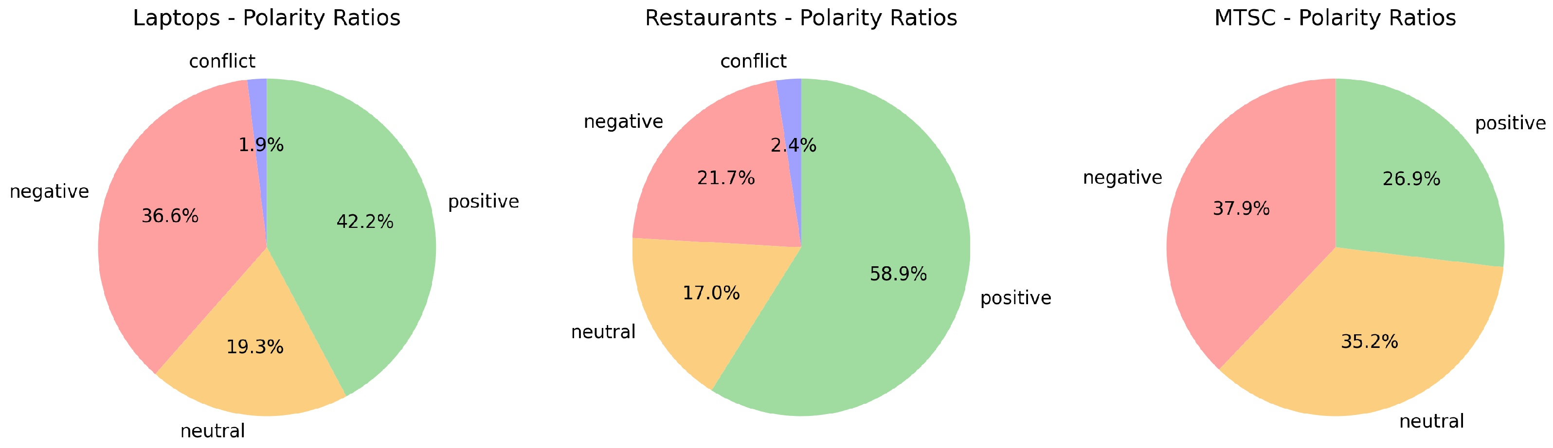
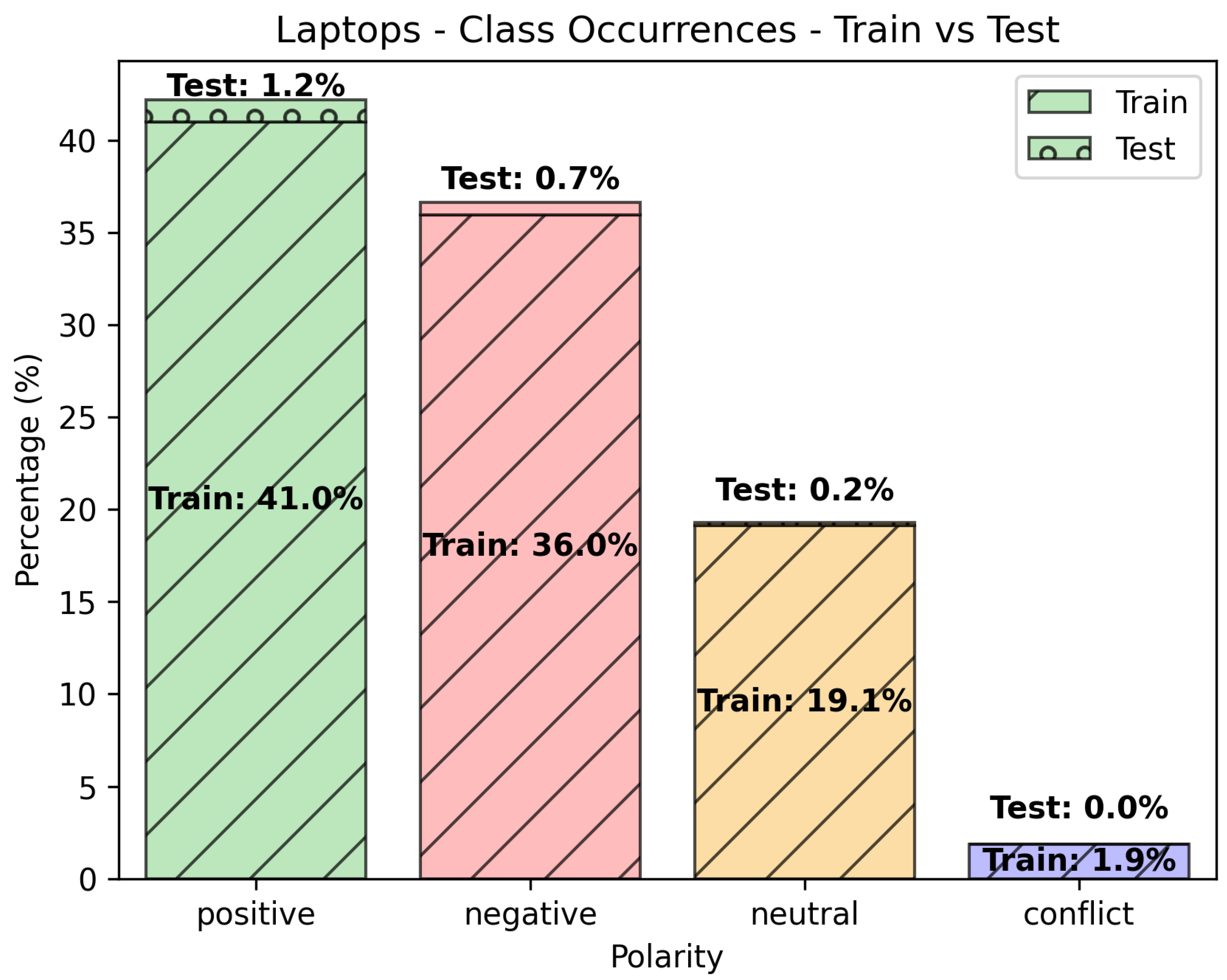
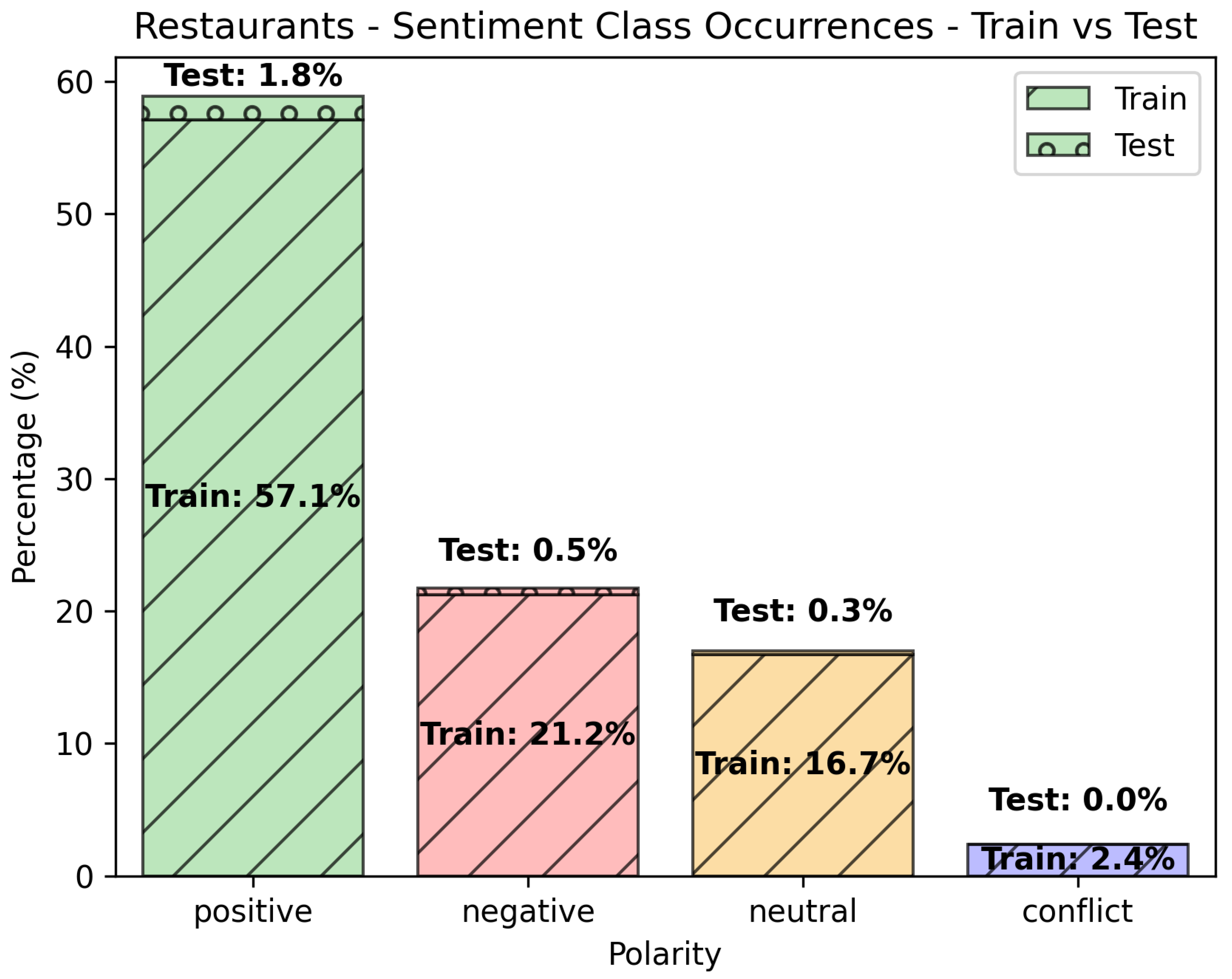
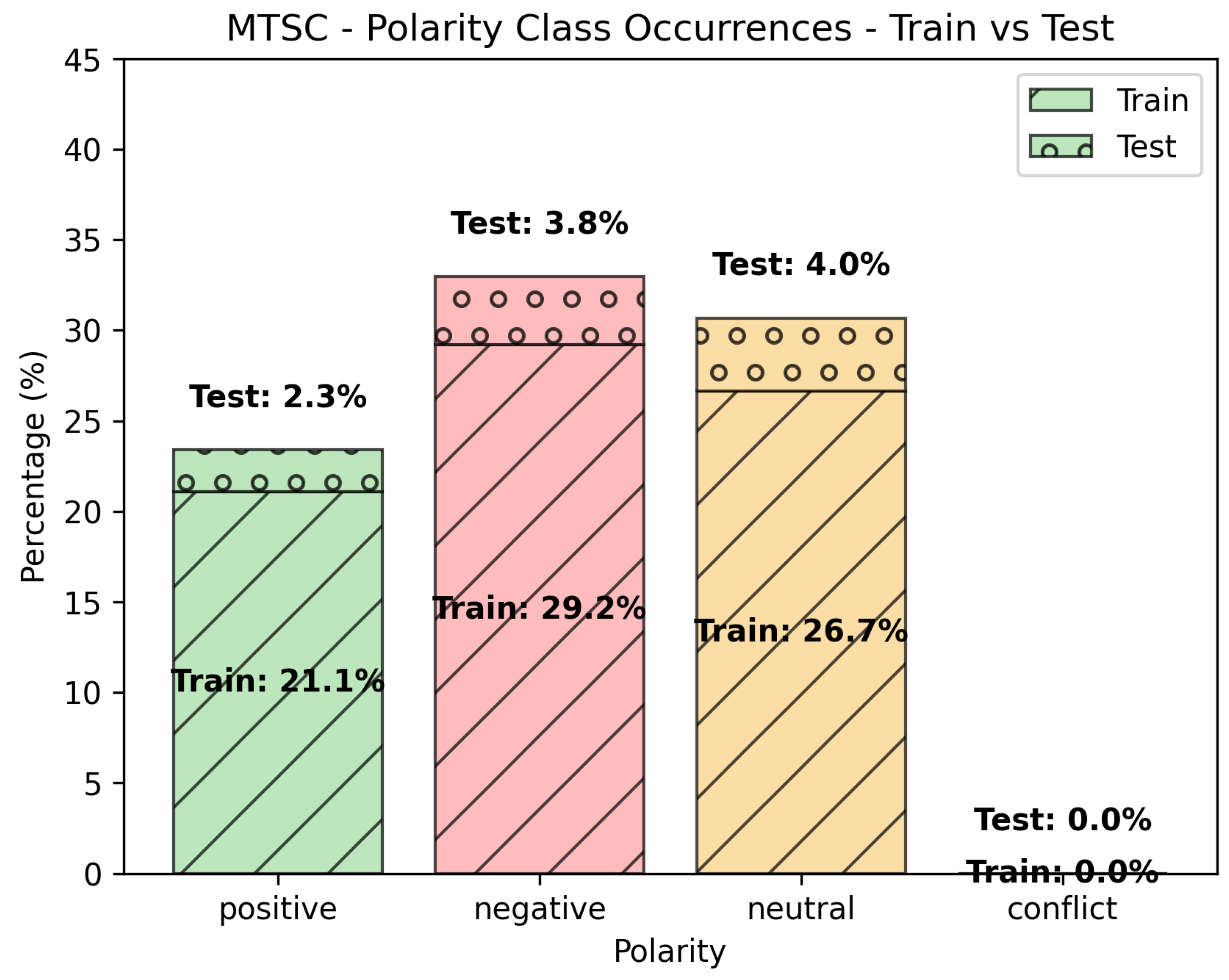
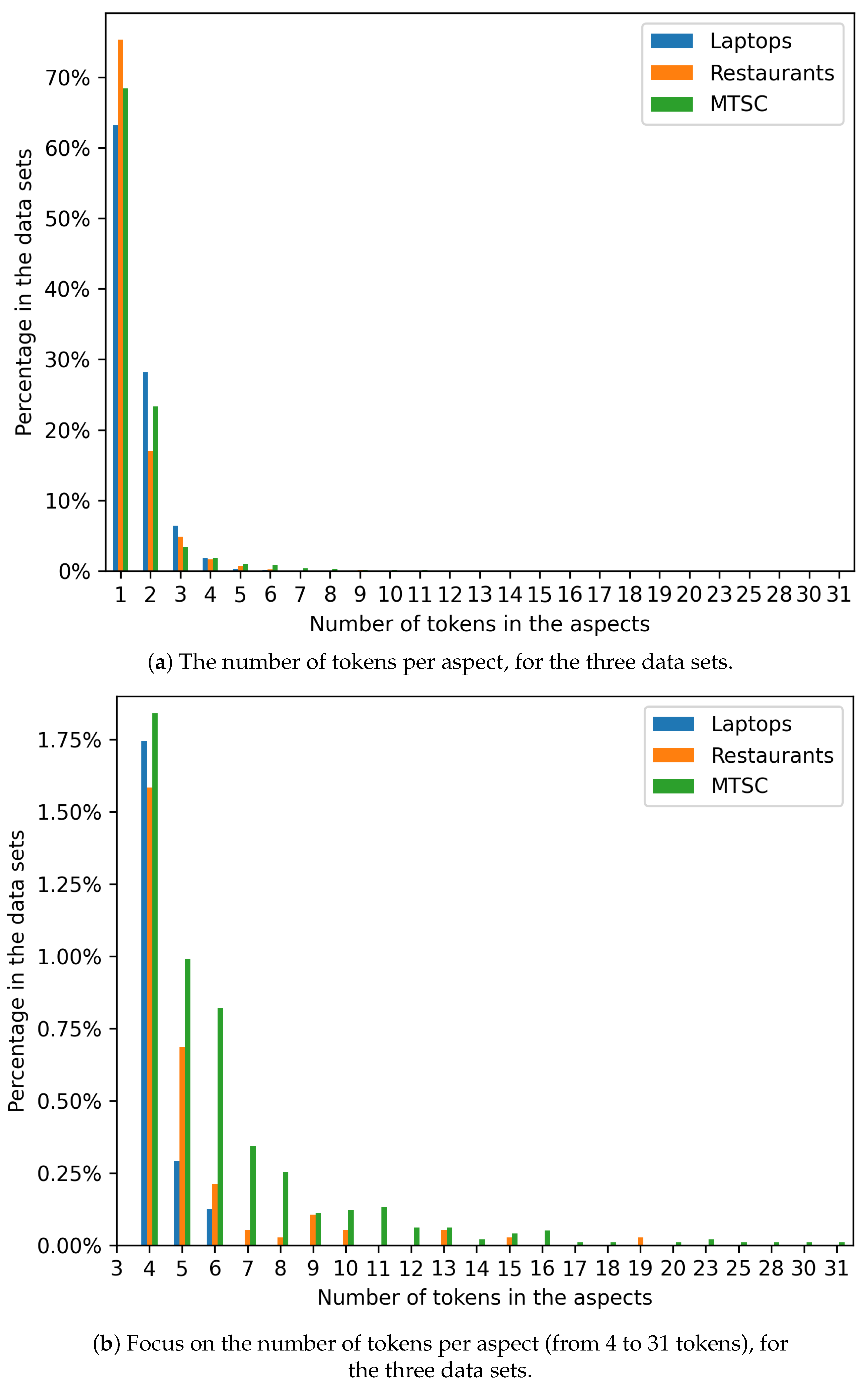
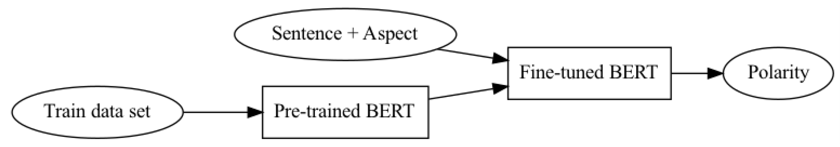
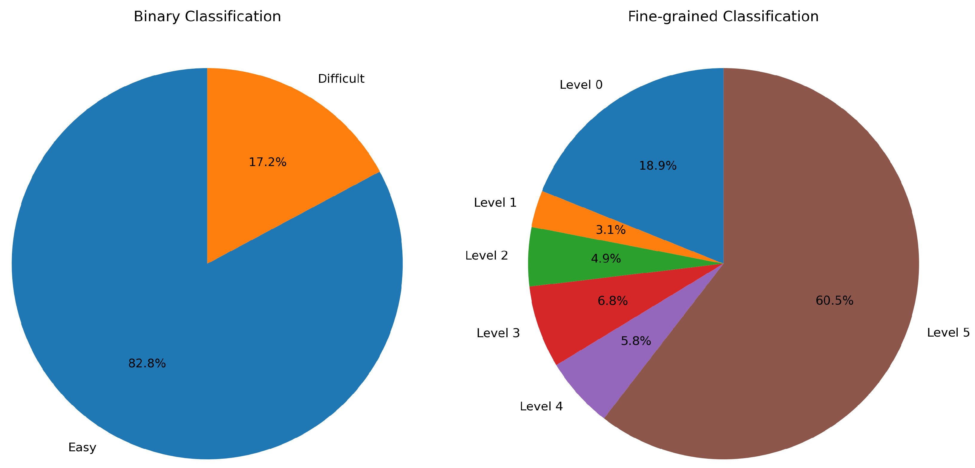
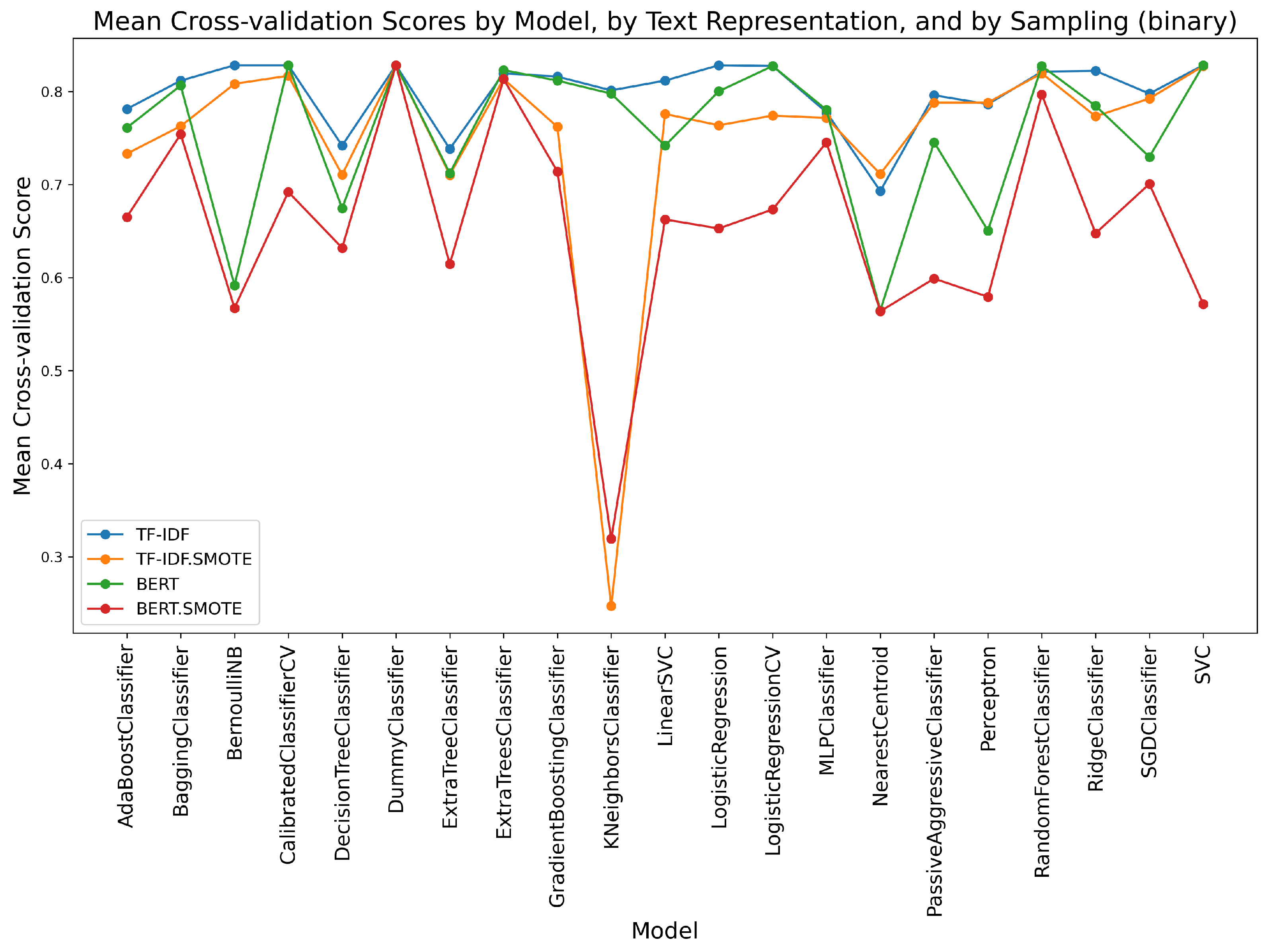
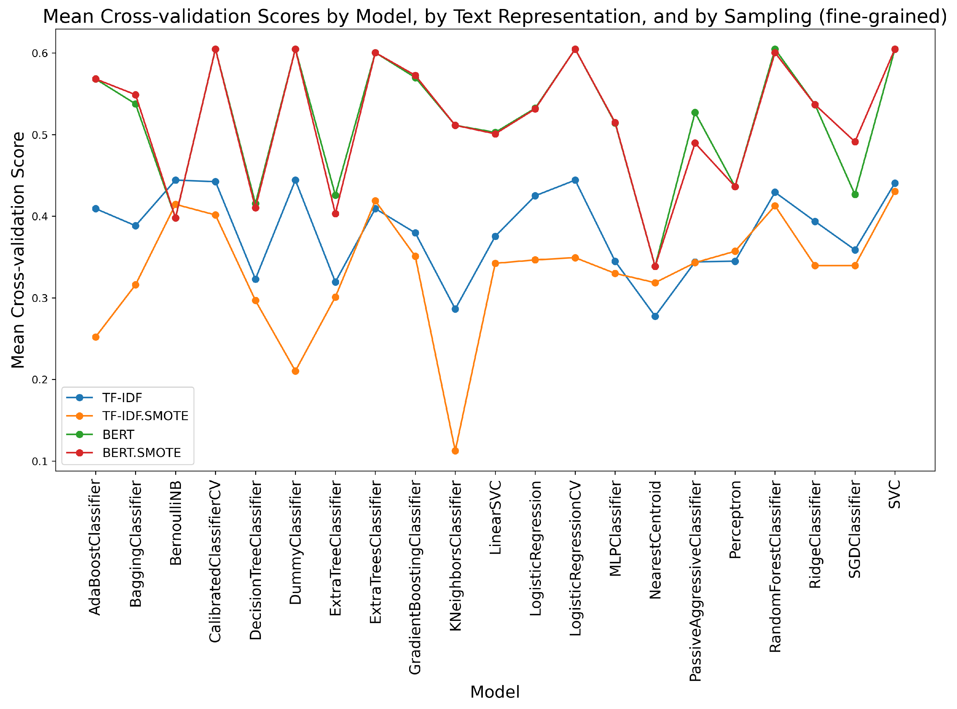
Table 1.
Summary of the data set information.
| Data Sets | Total | Train | Test | # of Classes |
|---|---|---|---|---|
| Laptops | 2407 | 2358 | 49 | 4 |
| Restaurants | 3789 | 3693 | 96 | 4 |
| MTSC | 9885 | 8739 | 1146 | 3 |
Table 2.
Token and sentence statistics for the data sets.
| Data Set | # of Observations | # of Unique Aspects | # of Unique Sentences | Max # of Tokens per Aspect |
|---|---|---|---|---|
| Laptops | 2407 | 1044 | 1484 | 6 |
| Restaurants | 3789 | 1289 | 2022 | 19 |
| MTSC | 9885 | 3525 | 8802 | 31 |
Table 3.
Average number of tokens, nouns, verbs, named entities, and adjectives per sentence.
| Data Set/Class | Tokens | Nouns | Verbs | Named Entities | Adjectives | |
|---|---|---|---|---|---|---|
| Laptops | Positive | 20.04 | 3.72 | 1.98 | 0.64 | 1.94 |
| Negative | 22.76 | 4.04 | 2.81 | 0.82 | 1.42 | |
| Neutral | 25.24 | 4.54 | 2.83 | 1.33 | 1.43 | |
| Conflict | 23.84 | 3.82 | 2.69 | 0.84 | 2.02 | |
| Restaurants | Positive | 18.81 | 3.77 | 1.41 | 0.54 | 2.20 |
| Negative | 22.50 | 4.10 | 2.18 | 0.50 | 1.99 | |
| Neutral | 21.62 | 4.14 | 2.26 | 0.74 | 1.48 | |
| Conflict | 22.31 | 3.60 | 1.76 | 0.48 | 2.67 | |
| MTSC | Positive | 30.12 | 5.07 | 3.29 | 2.95 | 1.99 |
| Negative | 31.58 | 5.31 | 3.55 | 3.27 | 1.94 | |
| Neutral | 27.63 | 4.13 | 3.03 | 3.30 | 1.40 | |
| Conflict | 0.00 | 0.00 | 0.00 | 0.00 | 0.00 | |
Table 4.
Hardware and software specifications.
| Hardware (Computing Cluster Node) | Specification |
|---|---|
| CPU | 40 Intel(R) Xeon(R) Silver 4114 CPU @ 2.20 GHz |
| RAM | 354 GB |
| GPU | 8 (7 Nvidia A40 and 1 Nvidia GeForce RTX 3090) |
| Software (Conda virtual environment) | Version |
| python | 3.11 |
| Python modules | Version |
| huggingface_hub | 0.14.1 |
| lazy-text-predict | 0.0.11 |
| lazypredict | 0.2.12 |
| lazytext | 0.0.2 |
| matplotlib-base | 3.7.1 |
| nltk | 3.7 |
| numpy | 1.24.3 |
| pandas | 1.3.5 |
| scikit-learn | 1.3.1 |
| scipy | 1.10.1 |
| spacy | 3.5.3 |
| torch | 2.0.1 |
| transformers | 4.29.2 |
Table 5.
Macro Metrics of Classification Models (“Laptops”, TF-IDF representations).
| Model | Precision (Macro) | Recall (Macro) | F1 (Macro) |
|---|---|---|---|
| AdaBoostClassifier | 0.351852 | 0.356681 | 0.333003 |
| BaggingClassifier | 0.734375 | 0.725754 | 0.729989 |
| BernoulliNB | 0.888616 | 0.613506 | 0.663075 |
| CalibratedClassifierCV | 0.968750 | 0.875000 | 0.913765 |
| DecisionTreeClassifier | 0.750000 | 0.734375 | 0.741935 |
| DummyClassifier | 0.197279 | 0.333333 | 0.247863 |
| ExtraTreeClassifier | 0.750000 | 0.734375 | 0.741935 |
| ExtraTreesClassifier | 0.750000 | 0.734375 | 0.741935 |
| GradientBoostingClassifier | 0.648674 | 0.542026 | 0.567858 |
| KNeighborsClassifier | 0.604725 | 0.544540 | 0.560063 |
| LinearSVC | 0.725000 | 0.656250 | 0.685855 |
| LogisticRegression | 0.783127 | 0.801006 | 0.786207 |
| LogisticRegressionCV | 0.620202 | 0.571839 | 0.584436 |
| MLPClassifier | 0.750000 | 0.734375 | 0.741935 |
| NearestCentroid | 0.410417 | 0.382543 | 0.377963 |
| PassiveAggressiveClassifier | 0.750000 | 0.734375 | 0.741935 |
| Perceptron | 0.700000 | 0.718750 | 0.705556 |
| RandomForestClassifier | 0.750000 | 0.734375 | 0.741935 |
| RidgeClassifier | 0.671371 | 0.640625 | 0.653305 |
| SGDClassifier | 0.725000 | 0.656250 | 0.685855 |
| SVC | 0.740385 | 0.717672 | 0.725551 |
Table 6.
Weighted Metrics of Classification Models (“Laptops”, TF-IDF representations).
| Model | Precision (Weighted) | Recall (Weighted) | F1 (Weighted) |
|---|---|---|---|
| AdaBoostClassifier | 0.695389 | 0.612245 | 0.615577 |
| BaggingClassifier | 0.979592 | 0.959184 | 0.969209 |
| BernoulliNB | 0.826355 | 0.795918 | 0.776692 |
| CalibratedClassifierCV | 0.944515 | 0.938776 | 0.937463 |
| DecisionTreeClassifier | 1.000000 | 0.979592 | 0.989467 |
| DummyClassifier | 0.350271 | 0.591837 | 0.440084 |
| ExtraTreeClassifier | 1.000000 | 0.979592 | 0.989467 |
| ExtraTreesClassifier | 1.000000 | 0.979592 | 0.989467 |
| GradientBoostingClassifier | 0.856602 | 0.795918 | 0.808693 |
| KNeighborsClassifier | 0.671202 | 0.673469 | 0.668267 |
| LinearSVC | 0.958503 | 0.938776 | 0.946707 |
| LogisticRegression | 0.859837 | 0.857143 | 0.854516 |
| LogisticRegressionCV | 0.738157 | 0.755102 | 0.734680 |
| MLPClassifier | 1.000000 | 0.979592 | 0.989467 |
| NearestCentroid | 0.684864 | 0.551020 | 0.602253 |
| PassiveAggressiveClassifier | 1.000000 | 0.979592 | 0.989467 |
| Perceptron | 0.983673 | 0.959184 | 0.969161 |
| RandomForestClassifier | 1.000000 | 0.979592 | 0.989467 |
| RidgeClassifier | 0.941409 | 0.918367 | 0.926085 |
| SGDClassifier | 0.958503 | 0.938776 | 0.946707 |
| SVC | 0.834969 | 0.836735 | 0.831855 |
Table 7.
Macro Metrics of Classification Models (“Restaurants”, TF-IDF representations).
| Model | Precision (Macro) | Recall (Macro) | F1 (Macro) |
|---|---|---|---|
| AdaBoostClassifier | 0.798309 | 0.413617 | 0.416818 |
| BaggingClassifier | 0.995169 | 0.981481 | 0.988043 |
| BernoulliNB | 0.828750 | 0.613617 | 0.672518 |
| CalibratedClassifierCV | 0.912913 | 0.791394 | 0.836613 |
| DecisionTreeClassifier | 1.000000 | 1.000000 | 1.000000 |
| DummyClassifier | 0.236111 | 0.333333 | 0.276423 |
| ExtraTreeClassifier | 1.000000 | 1.000000 | 1.000000 |
| ExtraTreesClassifier | 1.000000 | 1.000000 | 1.000000 |
| GradientBoostingClassifier | 0.936508 | 0.600000 | 0.674314 |
| KNeighborsClassifier | 0.724537 | 0.674292 | 0.696110 |
| LinearSVC | 0.924901 | 0.919826 | 0.920608 |
| LogisticRegression | 0.866234 | 0.702505 | 0.756657 |
| LogisticRegressionCV | 0.873585 | 0.819826 | 0.843531 |
| MLPClassifier | 1.000000 | 1.000000 | 1.000000 |
| NearestCentroid | 0.482186 | 0.450817 | 0.445678 |
| PassiveAggressiveClassifier | 0.930936 | 0.839542 | 0.879074 |
| Perceptron | 0.688576 | 0.700980 | 0.689108 |
| RandomForestClassifier | 1.000000 | 1.000000 | 1.000000 |
| RidgeClassifier | 0.924984 | 0.824728 | 0.865804 |
| SGDClassifier | 0.924901 | 0.919826 | 0.920608 |
| SVC | 0.933455 | 0.707407 | 0.771812 |
Table 8.
Weighted Metrics of Classification Models (“Restaurants”, TF-IDF representations).
| Model | Precision (Weighted) | Recall (Weighted) | F1 (Weighted) |
|---|---|---|---|
| AdaBoostClassifier | 0.772796 | 0.729167 | 0.645017 |
| BaggingClassifier | 0.989734 | 0.989583 | 0.989473 |
| BernoulliNB | 0.834485 | 0.833333 | 0.810978 |
| CalibratedClassifierCV | 0.915634 | 0.916667 | 0.910002 |
| DecisionTreeClassifier | 1.000000 | 1.000000 | 1.000000 |
| DummyClassifier | 0.501736 | 0.708333 | 0.587398 |
| ExtraTreeClassifier | 1.000000 | 1.000000 | 1.000000 |
| ExtraTreesClassifier | 1.000000 | 1.000000 | 1.000000 |
| GradientBoostingClassifier | 0.865079 | 0.833333 | 0.806849 |
| KNeighborsClassifier | 0.803964 | 0.812500 | 0.806575 |
| LinearSVC | 0.950264 | 0.947917 | 0.948238 |
| LogisticRegression | 0.873782 | 0.875000 | 0.862497 |
| LogisticRegressionCV | 0.913046 | 0.916667 | 0.913535 |
| MLPClassifier | 1.000000 | 1.000000 | 1.000000 |
| NearestCentroid | 0.824674 | 0.562500 | 0.650863 |
| PassiveAggressiveClassifier | 0.928760 | 0.927083 | 0.924641 |
| Perceptron | 0.965389 | 0.947917 | 0.953627 |
| RandomForestClassifier | 1.000000 | 1.000000 | 1.000000 |
| RidgeClassifier | 0.926900 | 0.927083 | 0.923168 |
| SGDClassifier | 0.950264 | 0.947917 | 0.948238 |
| SVC | 0.895795 | 0.885417 | 0.871685 |
Table 9.
Macro Metrics of Classification Models (“MTSC”, TF-IDF representations).
| Model | Precision (Macro) | Recall (Macro) | F1 (Macro) |
|---|---|---|---|
| AdaBoostClassifier | 0.536569 | 0.511031 | 0.511124 |
| BaggingClassifier | 0.546274 | 0.539847 | 0.542036 |
| BernoulliNB | 0.620338 | 0.609301 | 0.613077 |
| CalibratedClassifierCV | 0.598696 | 0.590106 | 0.591621 |
| DecisionTreeClassifier | 0.483979 | 0.483880 | 0.482779 |
| DummyClassifier | 0.124782 | 0.333333 | 0.181587 |
| ExtraTreeClassifier | 0.449816 | 0.446374 | 0.446124 |
| ExtraTreesClassifier | 0.610337 | 0.597893 | 0.601791 |
| GradientBoostingClassifier | 0.584919 | 0.547793 | 0.550139 |
| KNeighborsClassifier | 0.483402 | 0.473172 | 0.474578 |
| LinearSVC | 0.589215 | 0.584575 | 0.586015 |
| LogisticRegression | 0.605643 | 0.594484 | 0.597691 |
| LogisticRegressionCV | 0.609529 | 0.602939 | 0.605218 |
| MLPClassifier | 0.539425 | 0.537760 | 0.538246 |
| NearestCentroid | 0.480083 | 0.437883 | 0.416298 |
| PassiveAggressiveClassifier | 0.562594 | 0.558242 | 0.559689 |
| Perceptron | 0.569177 | 0.551341 | 0.554123 |
| RandomForestClassifier | 0.582065 | 0.564524 | 0.567516 |
| RidgeClassifier | 0.602595 | 0.597642 | 0.599191 |
| SGDClassifier | 0.599942 | 0.602576 | 0.600953 |
| SVC | 0.578846 | 0.562540 | 0.565638 |
Table 10.
Weighted Metrics of Classification Models (“MTSC”, TF-IDF representations).
| Model | Precision (Weighted) | Recall (Weighted) | F1 (Weighted) |
|---|---|---|---|
| AdaBoostClassifier | 0.544459 | 0.537522 | 0.527558 |
| BaggingClassifier | 0.556988 | 0.560209 | 0.557818 |
| BernoulliNB | 0.626705 | 0.629145 | 0.626609 |
| CalibratedClassifierCV | 0.610622 | 0.615183 | 0.610546 |
| DecisionTreeClassifier | 0.497215 | 0.496510 | 0.495555 |
| DummyClassifier | 0.140135 | 0.374346 | 0.203929 |
| ExtraTreeClassifier | 0.463308 | 0.465969 | 0.462460 |
| ExtraTreesClassifier | 0.617598 | 0.620419 | 0.617156 |
| GradientBoostingClassifier | 0.586393 | 0.586387 | 0.573521 |
| KNeighborsClassifier | 0.494559 | 0.500000 | 0.494082 |
| LinearSVC | 0.602032 | 0.605585 | 0.603095 |
| LogisticRegression | 0.614704 | 0.618674 | 0.614889 |
| LogisticRegressionCV | 0.621267 | 0.624782 | 0.622249 |
| MLPClassifier | 0.554007 | 0.556719 | 0.555062 |
| NearestCentroid | 0.500953 | 0.457243 | 0.430506 |
| PassiveAggressiveClassifier | 0.575761 | 0.579407 | 0.577021 |
| Perceptron | 0.578566 | 0.583770 | 0.576333 |
| RandomForestClassifier | 0.590895 | 0.595986 | 0.588793 |
| RidgeClassifier | 0.615804 | 0.619546 | 0.616933 |
| SGDClassifier | 0.617770 | 0.615183 | 0.616206 |
| SVC | 0.587705 | 0.592496 | 0.586000 |
Table 11.
Macro Metrics of Classification Models (“Laptops”, BERT representations).
| Model | Precision (Macro) | Recall (Macro) | F1 (Macro) |
|---|---|---|---|
| AdaBoostClassifier | 0.811111 | 0.597701 | 0.628514 |
| BaggingClassifier | 0.750000 | 0.734375 | 0.741935 |
| BernoulliNB | 0.579808 | 0.550647 | 0.563304 |
| CalibratedClassifierCV | 0.956944 | 0.884339 | 0.914598 |
| DecisionTreeClassifier | 0.741667 | 0.718750 | 0.729096 |
| DummyClassifier | 0.197279 | 0.333333 | 0.247863 |
| ExtraTreeClassifier | 0.750000 | 0.734375 | 0.741935 |
| ExtraTreesClassifier | 0.750000 | 0.734375 | 0.741935 |
| GradientBoostingClassifier | 0.741667 | 0.671875 | 0.701984 |
| KNeighborsClassifier | 0.707283 | 0.713362 | 0.709995 |
| LinearSVC | 0.967672 | 0.967672 | 0.967672 |
| LogisticRegression | 0.915535 | 0.738506 | 0.794381 |
| LogisticRegressionCV | 0.866071 | 0.778017 | 0.814312 |
| MLPClassifier | 0.988889 | 0.979167 | 0.983598 |
| NearestCentroid | 0.443548 | 0.394397 | 0.414286 |
| PassiveAggressiveClassifier | 0.752381 | 0.729167 | 0.686800 |
| Perceptron | 0.703680 | 0.808190 | 0.705096 |
| RandomForestClassifier | 0.750000 | 0.734375 | 0.741935 |
| RidgeClassifier | 0.915323 | 0.768678 | 0.813889 |
| SGDClassifier | 0.700893 | 0.692888 | 0.696820 |
| SVC | 0.840404 | 0.611351 | 0.649462 |
Table 12.
Weighted Metrics of Classification Models (“Laptops”, BERT representations).
| Model | Precision (Weighted) | Recall (Weighted) | F1 (Weighted) |
|---|---|---|---|
| AdaBoostClassifier | 0.753061 | 0.734694 | 0.724577 |
| BaggingClassifier | 1.000000 | 0.979592 | 0.989467 |
| BernoulliNB | 0.785871 | 0.755102 | 0.767912 |
| CalibratedClassifierCV | 0.940136 | 0.938776 | 0.937837 |
| DecisionTreeClassifier | 0.980272 | 0.959184 | 0.968200 |
| DummyClassifier | 0.350271 | 0.591837 | 0.440084 |
| ExtraTreeClassifier | 1.000000 | 0.979592 | 0.989467 |
| ExtraTreesClassifier | 1.000000 | 0.979592 | 0.989467 |
| GradientBoostingClassifier | 0.980272 | 0.959184 | 0.967774 |
| KNeighborsClassifier | 0.797805 | 0.795918 | 0.796472 |
| LinearSVC | 0.959184 | 0.959184 | 0.959184 |
| LogisticRegression | 0.870440 | 0.857143 | 0.850731 |
| LogisticRegressionCV | 0.819060 | 0.816327 | 0.813943 |
| MLPClassifier | 0.980272 | 0.979592 | 0.979436 |
| NearestCentroid | 0.703094 | 0.673469 | 0.683382 |
| PassiveAggressiveClassifier | 0.851895 | 0.795918 | 0.779637 |
| Perceptron | 0.828240 | 0.775510 | 0.783489 |
| RandomForestClassifier | 1.000000 | 0.979592 | 0.989467 |
| RidgeClassifier | 0.882818 | 0.877551 | 0.872789 |
| SGDClassifier | 0.916910 | 0.897959 | 0.907268 |
| SVC | 0.787384 | 0.775510 | 0.760764 |
Table 13.
Macro Metrics of Classification Models (“Restaurants”, BERT representations).
| Model | Precision (Macro) | Recall (Macro) | F1 (Macro) |
|---|---|---|---|
| AdaBoostClassifier | 0.537594 | 0.456618 | 0.486397 |
| BaggingClassifier | 1.000000 | 1.000000 | 1.000000 |
| BernoulliNB | 0.512220 | 0.512418 | 0.508235 |
| CalibratedClassifierCV | 0.909456 | 0.585185 | 0.641217 |
| DecisionTreeClassifier | 1.000000 | 1.000000 | 1.000000 |
| DummyClassifier | 0.236111 | 0.333333 | 0.276423 |
| ExtraTreeClassifier | 1.000000 | 1.000000 | 1.000000 |
| ExtraTreesClassifier | 1.000000 | 1.000000 | 1.000000 |
| GradientBoostingClassifier | 0.968889 | 0.811111 | 0.870047 |
| KNeighborsClassifier | 0.718704 | 0.645861 | 0.674860 |
| LinearSVC | 0.926190 | 0.640741 | 0.688251 |
| LogisticRegression | 0.891105 | 0.598802 | 0.647447 |
| LogisticRegressionCV | 0.903175 | 0.566667 | 0.623642 |
| MLPClassifier | 0.923077 | 0.985294 | 0.949003 |
| NearestCentroid | 0.512138 | 0.395915 | 0.425557 |
| PassiveAggressiveClassifier | 0.879584 | 0.511111 | 0.563584 |
| Perceptron | 0.727431 | 0.720153 | 0.716450 |
| RandomForestClassifier | 1.000000 | 1.000000 | 1.000000 |
| RidgeClassifier | 0.918724 | 0.637037 | 0.702541 |
| SGDClassifier | 0.780556 | 0.529630 | 0.578348 |
| SVC | 0.900000 | 0.533333 | 0.571188 |
Table 14.
Weighted Metrics of Classification Models (“Restaurants”, BERT representations).
| Model | Precision (Weighted) | Recall (Weighted) | F1 (Weighted) |
|---|---|---|---|
| AdaBoostClassifier | 0.787320 | 0.791667 | 0.781311 |
| BaggingClassifier | 1.000000 | 1.000000 | 1.000000 |
| BernoulliNB | 0.778746 | 0.739583 | 0.756588 |
| CalibratedClassifierCV | 0.854942 | 0.833333 | 0.802002 |
| DecisionTreeClassifier | 1.000000 | 1.000000 | 1.000000 |
| DummyClassifier | 0.501736 | 0.708333 | 0.587398 |
| ExtraTreeClassifier | 1.000000 | 1.000000 | 1.000000 |
| ExtraTreesClassifier | 1.000000 | 1.000000 | 1.000000 |
| GradientBoostingClassifier | 0.933889 | 0.927083 | 0.922239 |
| KNeighborsClassifier | 0.800064 | 0.812500 | 0.802541 |
| LinearSVC | 0.880357 | 0.864583 | 0.837967 |
| LogisticRegression | 0.848726 | 0.833333 | 0.804811 |
| LogisticRegressionCV | 0.846329 | 0.822917 | 0.789030 |
| MLPClassifier | 0.975962 | 0.968750 | 0.970436 |
| NearestCentroid | 0.800187 | 0.614583 | 0.682193 |
| PassiveAggressiveClassifier | 0.818521 | 0.791667 | 0.746228 |
| Perceptron | 0.810547 | 0.791667 | 0.797258 |
| RandomForestClassifier | 1.000000 | 1.000000 | 1.000000 |
| RidgeClassifier | 0.870692 | 0.854167 | 0.832109 |
| SGDClassifier | 0.800174 | 0.802083 | 0.762642 |
| SVC | 0.839583 | 0.812500 | 0.769105 |
Table 15.
Macro Metrics of Classification Models (“MTSC”, BERT representations).
| Model | Precision (Macro) | Recall (Macro) | F1 (Macro) |
|---|---|---|---|
| AdaBoostClassifier | 0.617579 | 0.607600 | 0.611387 |
| BaggingClassifier | 0.583002 | 0.570900 | 0.574723 |
| BernoulliNB | 0.594007 | 0.599098 | 0.594284 |
| CalibratedClassifierCV | 0.717618 | 0.697904 | 0.704669 |
| DecisionTreeClassifier | 0.502683 | 0.506414 | 0.503590 |
| DummyClassifier | 0.124782 | 0.333333 | 0.181587 |
| ExtraTreeClassifier | 0.420560 | 0.422548 | 0.420626 |
| ExtraTreesClassifier | 0.652450 | 0.637024 | 0.641867 |
| GradientBoostingClassifier | 0.674504 | 0.659606 | 0.664726 |
| KNeighborsClassifier | 0.575093 | 0.552326 | 0.554446 |
| LinearSVC | 0.706773 | 0.694961 | 0.699503 |
| LogisticRegression | 0.719955 | 0.700226 | 0.707067 |
| LogisticRegressionCV | 0.726826 | 0.700067 | 0.708159 |
| MLPClassifier | 0.692743 | 0.686242 | 0.688107 |
| NearestCentroid | 0.574224 | 0.574224 | 0.574224 |
| PassiveAggressiveClassifier | 0.657355 | 0.629713 | 0.582214 |
| Perceptron | 0.630884 | 0.547369 | 0.446289 |
| RandomForestClassifier | 0.670888 | 0.659953 | 0.663928 |
| RidgeClassifier | 0.710743 | 0.692509 | 0.698889 |
| SGDClassifier | 0.687735 | 0.672053 | 0.659408 |
| SVC | 0.720193 | 0.690442 | 0.698967 |
Table 16.
Weighted Metrics of Classification Models (“MTSC”, BERT representations).
| Model | Precision (Weighted) | Recall (Weighted) | F1 (Weighted) |
|---|---|---|---|
| AdaBoostClassifier | 0.619690 | 0.620419 | 0.619124 |
| BaggingClassifier | 0.587681 | 0.589878 | 0.587083 |
| BernoulliNB | 0.607692 | 0.602094 | 0.602517 |
| CalibratedClassifierCV | 0.718311 | 0.718150 | 0.715857 |
| DecisionTreeClassifier | 0.518598 | 0.513089 | 0.515090 |
| DummyClassifier | 0.140135 | 0.374346 | 0.203929 |
| ExtraTreeClassifier | 0.437334 | 0.431065 | 0.433455 |
| ExtraTreesClassifier | 0.654367 | 0.655323 | 0.652600 |
| GradientBoostingClassifier | 0.678232 | 0.679756 | 0.677239 |
| KNeighborsClassifier | 0.578520 | 0.575916 | 0.568944 |
| LinearSVC | 0.710757 | 0.710297 | 0.709302 |
| LogisticRegression | 0.720905 | 0.719895 | 0.717951 |
| LogisticRegressionCV | 0.726504 | 0.724258 | 0.721086 |
| MLPClassifier | 0.696425 | 0.696335 | 0.694988 |
| NearestCentroid | 0.579407 | 0.579407 | 0.579407 |
| PassiveAggressiveClassifier | 0.674502 | 0.608202 | 0.570665 |
| Perceptron | 0.648515 | 0.521815 | 0.417314 |
| RandomForestClassifier | 0.676899 | 0.678883 | 0.676761 |
| RidgeClassifier | 0.712000 | 0.712042 | 0.709899 |
| SGDClassifier | 0.698238 | 0.672775 | 0.661620 |
| SVC | 0.717385 | 0.715532 | 0.711701 |
Table 17.
Classification report for fine-tuned BERT (“Laptops”).
| Model | Precision | Recall | F1-Score | Support |
|---|---|---|---|---|
| negative | 0.97 | 0.97 | 0.97 | 29 |
| neutral | 1.00 | 0.88 | 0.93 | 16 |
| positive | 0.67 | 1.00 | 0.80 | 4 |
| conflict | 0.00 | 0.00 | 0.00 | 0 |
| Accuracy | - | - | 0.94 | 49 |
| Weighted Avg | 0.88 | 0.95 | 0.90 | 49 |
| Macro Avg | 0.95 | 0.94 | 0.94 | 49 |
Table 18.
Classification report for fine-tuned BERT (“Restaurants”).
| Model | Precision | Recall | F1-Score | Support |
|---|---|---|---|---|
| negative | 0.89 | 0.99 | 0.94 | 68 |
| neutral | 1.00 | 0.50 | 0.67 | 18 |
| positive | 0.64 | 0.70 | 0.67 | 10 |
| conflict | 0.00 | 0.00 | 0.00 | 0 |
| Accuracy | - | - | 0.86 | 96 |
| Weighted Avg | 0.63 | 0.55 | 0.57 | 96 |
| Macro Avg | 0.89 | 0.86 | 0.86 | 96 |
Table 19.
Classification report for fine-tuned BERT (“MTSC”).
| Model | Precision | Recall | F1-Score | Support |
|---|---|---|---|---|
| negative | 0.57 | 0.79 | 0.66 | 262 |
| neutral | 0.93 | 0.68 | 0.79 | 429 |
| positive | 0.72 | 0.75 | 0.73 | 455 |
| Accuracy | - | - | 0.73 | 1146 |
| Weighted Avg | 0.74 | 0.74 | 0.73 | 1146 |
| Macro Avg | 0.77 | 0.73 | 0.74 | 1146 |
Table 20.
Classification Report for Majority Vote (“Laptops”, TF-IDF representations, all models).
| Model | Precision | Recall | F1-Score | Support |
|---|---|---|---|---|
| conflict | 0.00 | 0.00 | 0.00 | 0 |
| negative | 1.00 | 0.88 | 0.93 | 16 |
| neutral | 1.00 | 1.00 | 1.00 | 4 |
| positive | 0.97 | 1.00 | 0.98 | 29 |
| Accuracy | - | - | 0.96 | 49 |
| Weighted Avg | 0.98 | 0.96 | 0.97 | 49 |
| Macro Avg | 0.74 | 0.72 | 0.73 | 49 |
Table 21.
Top five models with respect to accuracy (“Laptops”, TF-IDF representations).
| Model | Accuracy |
|---|---|
| DecisionTreeClassifier | 0.9796 |
| ExtraTreeClassifier | 0.9796 |
| ExtraTreesClassifier | 0.9796 |
| MLPClassifier | 0.9796 |
| PassiveAggressiveClassifier | 0.9796 |
Table 22.
Classification report for majority vote (“Laptops”, TF-IDF representations, top five models).
Table 22.
Classification report for majority vote (“Laptops”, TF-IDF representations, top five models).
| Model | Precision | Recall | F1-Score | Support |
|---|---|---|---|---|
| conflict | 0.00 | 0.00 | 0.00 | 0 |
| negative | 1.00 | 0.94 | 0.97 | 16 |
| neutral | 1.00 | 1.00 | 1.00 | 4 |
| positive | 1.00 | 1.00 | 1.00 | 29 |
| Accuracy | - | - | 0.98 | 49 |
| Weighted Avg | 1.00 | 0.98 | 0.99 | 49 |
| Macro Avg | 0.75 | 0.73 | 0.74 | 49 |
Table 23.
Classification Report for Majority Vote (“Restaurants”, TF-IDF representations, all models).
Table 23.
Classification Report for Majority Vote (“Restaurants”, TF-IDF representations, all models).
| Model | Precision | Recall | F1-Score | Support |
|---|---|---|---|---|
| negative | 1.00 | 0.89 | 0.94 | 18 |
| neutral | 1.00 | 0.90 | 0.95 | 10 |
| positive | 0.96 | 1.00 | 0.98 | 68 |
| Accuracy | - | - | 0.97 | 96 |
| Weighted Avg | 0.97 | 0.97 | 0.97 | 96 |
| Macro Avg | 0.99 | 0.93 | 0.96 | 96 |
Table 24.
Top five models with respect to accuracy (“Restaurants”, TF-IDF representations).
| Model | Accuracy |
|---|---|
| DecisionTreeClassifier | 1.0000 |
| ExtraTreeClassifier | 1.0000 |
| ExtraTreesClassifier | 1.0000 |
| MLPClassifier | 1.0000 |
| RandomForestClassifier | 1.0000 |
Table 25.
Classification report for majority vote (“Restaurants”, TF-IDF representations, top 5 models).
Table 25.
Classification report for majority vote (“Restaurants”, TF-IDF representations, top 5 models).
| Model | Precision | Recall | F1-Score | Support |
|---|---|---|---|---|
| negative | 1.00 | 1.00 | 1.00 | 18 |
| neutral | 1.00 | 1.00 | 1.00 | 10 |
| positive | 1.00 | 1.00 | 1.00 | 68 |
| Accuracy | - | - | 1.00 | 96 |
| Weighted Avg | 1.00 | 1.00 | 1.00 | 96 |
| Macro Avg | 1.00 | 1.00 | 1.00 | 96 |
Table 26.
Classification Report for Majority Vote (“MTSC”, TF-IDF representations, all models).
| Model | Precision | Recall | F1-Score | Support |
|---|---|---|---|---|
| negative | 0.64 | 0.67 | 0.66 | 429 |
| neutral | 0.62 | 0.69 | 0.65 | 455 |
| positive | 0.59 | 0.43 | 0.50 | 262 |
| Accuracy | - | - | 0.62 | 1146 |
| Weighted Avg | 0.62 | 0.62 | 0.62 | 1146 |
| Macro Avg | 0.62 | 0.60 | 0.60 | 1146 |
Table 27.
Top five models with respect to accuracy (“MTSC”, TF-IDF representations).
| Model | Accuracy |
|---|---|
| BernoulliNB | 0.6291 |
| LogisticRegressionCV | 0.6248 |
| ExtraTreesClassifier | 0.6204 |
| RidgeClassifier | 0.6195 |
| LogisticRegression | 0.6187 |
Table 28.
Classification Report for Majority Vote (“MTSC”, TF-IDF representations, top 5 models).
| Model | Precision | Recall | F1-Score | Support |
|---|---|---|---|---|
| negative | 0.65 | 0.70 | 0.67 | 429 |
| neutral | 0.64 | 0.66 | 0.65 | 455 |
| positive | 0.56 | 0.45 | 0.50 | 262 |
| Accuracy | - | - | 0.63 | 1146 |
| Weighted Avg | 0.62 | 0.63 | 0.62 | 1146 |
| Macro Avg | 0.61 | 0.60 | 0.61 | 1146 |
Table 29.
Classification Report for Majority Vote (“Laptops”, BERT representations, all models).
| Model | Precision | Recall | F1-Score | Support |
|---|---|---|---|---|
| conflict | 0.00 | 0.00 | 0.00 | 0 |
| negative | 1.00 | 0.81 | 0.90 | 16 |
| neutral | 1.00 | 0.75 | 0.86 | 4 |
| positive | 0.91 | 1.00 | 0.95 | 29 |
| Accuracy | - | - | 0.92 | 49 |
| Weighted Avg | 0.94 | 0.92 | 0.93 | 49 |
| Macro Avg | 0.73 | 0.64 | 0.68 | 49 |
Table 30.
Top five models with respect to accuracy (“Laptops”, BERT representations).
| Model | Accuracy |
|---|---|
| ExtraTreesClassifier | 0.9796 |
| RandomForestClassifier | 0.9796 |
| DecisionTreeClassifier | 0.9592 |
| ExtraTreeClassifier | 0.9592 |
| GradientBoostingClassifier | 0.9592 |
Table 31.
Classification Report for Majority Vote (“Laptops”, BERT representations, top five models).
Table 31.
Classification Report for Majority Vote (“Laptops”, BERT representations, top five models).
| Model | Precision | Recall | F1-Score | Support |
|---|---|---|---|---|
| conflict | 0.00 | 0.00 | 0.00 | 0 |
| negative | 1.00 | 0.94 | 0.97 | 16 |
| neutral | 1.00 | 1.00 | 1.00 | 4 |
| positive | 1.00 | 1.00 | 1.00 | 29 |
| Accuracy | - | - | 0.98 | 49 |
| Weighted Avg | 1.00 | 0.98 | 0.99 | 49 |
| Macro Avg | 0.75 | 0.73 | 0.74 | 49 |
Table 32.
Classification Report for Majority Vote (“Restaurants”, BERT representations, all models).
Table 32.
Classification Report for Majority Vote (“Restaurants”, BERT representations, all models).
| Model | Precision | Recall | F1-Score | Support |
|---|---|---|---|---|
| negative | 0.92 | 0.61 | 0.73 | 18 |
| neutral | 1.00 | 0.30 | 0.46 | 10 |
| positive | 0.84 | 1.00 | 0.91 | 68 |
| Accuracy | - | - | 0.85 | 96 |
| Weighted Avg | 0.87 | 0.85 | 0.83 | 96 |
| Macro Avg | 0.92 | 0.64 | 0.70 | 96 |
Table 33.
Top five models with respect to accuracy (“Restaurants”, BERT representations).
| Model | Accuracy |
|---|---|
| BaggingClassifier | 1.0000 |
| DecisionTreeClassifier | 1.0000 |
| ExtraTreeClassifier | 1.0000 |
| ExtraTreesClassifier | 1.0000 |
| RandomForestClassifier | 1.0000 |
Table 34.
Classification Report for Majority Vote (“Restaurants”, BERT representations, top five models).
Table 34.
Classification Report for Majority Vote (“Restaurants”, BERT representations, top five models).
| Model | Precision | Recall | F1-Score | Support |
|---|---|---|---|---|
| negative | 1.00 | 1.00 | 1.00 | 18 |
| neutral | 1.00 | 1.00 | 1.00 | 10 |
| positive | 1.00 | 1.00 | 1.00 | 68 |
| Accuracy | - | - | 1.00 | 96 |
| Weighted Avg | 1.00 | 1.00 | 1.00 | 96 |
| Macro Avg | 1.00 | 1.00 | 1.00 | 96 |
Table 35.
Classification Report for Majority Vote (“MTSC”, BERT representations, all models).
| Model | Precision | Recall | F1-Score | Support |
|---|---|---|---|---|
| negative | 0.71 | 0.84 | 0.77 | 429 |
| neutral | 0.75 | 0.70 | 0.73 | 455 |
| positive | 0.71 | 0.58 | 0.64 | 262 |
| Accuracy | - | - | 0.73 | 1146 |
| Weighted Avg | 0.73 | 0.73 | 0.72 | 1146 |
| Macro Avg | 0.72 | 0.71 | 0.71 | 1146 |
Table 36.
Top five models with respect to accuracy (“MTSC”, BERT representations).
| Model | Accuracy |
|---|---|
| LogisticRegressionCV | 0.7243 |
| LogisticRegression | 0.7199 |
| CalibratedClassifierCV | 0.7182 |
| SVC | 0.7155 |
| RidgeClassifier | 0.7120 |
Table 37.
Classification Report for Majority Vote (“MTSC”, BERT representations, top five models).
| Model | Precision | Recall | F1-Score | Support |
|---|---|---|---|---|
| negative | 0.76 | 0.77 | 0.76 | 429 |
| neutral | 0.70 | 0.79 | 0.75 | 455 |
| positive | 0.73 | 0.57 | 0.64 | 262 |
| Accuracy | - | - | 0.73 | 1146 |
| Weighted Avg | 0.73 | 0.73 | 0.73 | 1146 |
| Macro Avg | 0.73 | 0.71 | 0.72 | 1146 |
Table 38.
Selected sentences from the “MTSC” data set that were wrongly classified by the majority vote, with ChatGPT predicted polarities. The wrong predictions are in bold.
Table 38.
Selected sentences from the “MTSC” data set that were wrongly classified by the majority vote, with ChatGPT predicted polarities. The wrong predictions are in bold.
| Sentence | Aspect | True Polarity | ChatGPT Polarity |
|---|---|---|---|
| In an atmosphere where some delegates remain anti-Trump and party leaders like Paul Ryan are barely mentioning Trump in their speeches, Hillary Clinton is a unifying force. | Hillary Clinton | positive | positive |
| A new presidential cabinet will be formed as well as a national reconciliation committee, which will include youth movements that have been behind anti-Morsi demonstrations. | Morsi | negative | negative |
| His persona is generally adult. | His | positive | neutral |
| The more left wing candidate for deputy leader—Julie Morgan, widow of former first minister of Wales, Rhodri—was defeated by Carolyn Harris at the party’s spring conference. | Carolyn Harris | positive | positive |
| In a statement Saturday, London Moore, the president of the Theta Gamma chapter of Delta Delta Delta, condemned the “racist, offensive and disgraceful” behavior seen in the video. | London Moore, the president of the Theta Gamma chapter of Delta Delta Delta | positive | positive |
| President Muhammadu Buhari was poised to win a second term despite falling short on promises to recharge the economy and defeat the Boko Haram insurgents. | President Muhammadu Buhari | negative | neutral |
Disclaimer/Publisher’s Note: The statements, opinions and data contained in all publications are solely those of the individual author(s) and contributor(s) and not of MDPI and/or the editor(s). MDPI and/or the editor(s) disclaim responsibility for any injury to people or property resulting from any ideas, methods, instructions or products referred to in the content. |
© 2023 by the authors. Licensee MDPI, Basel, Switzerland. This article is an open access article distributed under the terms and conditions of the Creative Commons Attribution (CC BY) license (https://creativecommons.org/licenses/by/4.0/).
Share and Cite
MDPI and ACS Style
Chifu, A.-G.; Fournier, S. Sentiment Difficulty in Aspect-Based Sentiment Analysis. Mathematics 2023, 11, 4647. https://doi.org/10.3390/math11224647
AMA Style
Chifu A-G, Fournier S. Sentiment Difficulty in Aspect-Based Sentiment Analysis. Mathematics. 2023; 11(22):4647. https://doi.org/10.3390/math11224647
Chicago/Turabian StyleChifu, Adrian-Gabriel, and Sébastien Fournier. 2023. "Sentiment Difficulty in Aspect-Based Sentiment Analysis" Mathematics 11, no. 22: 4647. https://doi.org/10.3390/math11224647
Note that from the first issue of 2016, this journal uses article numbers instead of page numbers. See further details here.