Article

Application of Advanced Optimized Soft Computing Models for Atmospheric Variable Forecasting

by
Rana Muhammad Adnan
1,
Sarita Gajbhiye Meshram
2,
Reham R. Mostafa
3,
Abu Reza Md. Towfiqul Islam
4,*,
S. I. Abba
5,
Francis Andorful
6 and
Zhihuan Chen
7,*
1
School of Economics and Statistics, Guangzhou University, Guangzhou 510006, China
2
Water Resources and Applied Mathematics Research Lab, Nagpur 440027, India
3
Information Systems Department, Faculty of Computers and Information Sciences, Mansoura University, Mansoura 35516, Egypt
4
Department of Disaster Management, Begum Rokeya University, Rangpur 5400, Bangladesh
5
Interdisciplinary Research Center for Membranes and Water Security, King Fahd University of Petroleum & Minerals, Dhahran 31261, Saudi Arabia
6
Department of Geography and Resource Development, University of Ghana, Accra 23321, Ghana
7
Engineering Research Center for Metallurgical Automation and Measurement Technology of Ministry of Education, Wuhan University of Science and Technology, Wuhan 431400, China
*
Authors to whom correspondence should be addressed.
Mathematics 2023, 11(5), 1213; https://doi.org/10.3390/math11051213
Submission received: 19 December 2022 / Revised: 17 February 2023 / Accepted: 27 February 2023 / Published: 1 March 2023
(This article belongs to the Special Issue Advanced Optimization Methods and Applications)

Abstract

:
Precise Air temperature modeling is crucial for a sustainable environment. In this study, a novel binary optimized machine learning model, the random vector functional link (RVFL) with the integration of Moth Flame Optimization Algorithm (MFO) and Water Cycle Optimization Algorithm (WCA) is examined to estimate the monthly and daily temperature time series of Rajshahi Climatic station in Bangladesh. Various combinations of temperature and precipitation were used to predict the temperature time series. The prediction ability of the novel binary optimized machine learning model (RVFL-WCAMFO) is compared with the single optimized machine learning models (RVFL-WCA and RVFL-MFO) and the standalone machine learning model (RVFL). Root mean square errors (RMSE), the mean absolute error (MAE), the Nash–Sutcliffe efficiency (NSE), and the determination coefficient (R2) statistical indexes were utilized to access the prediction ability of the selected models. The proposed binary optimized machine learning model (RVFL-WCAMFO) outperformed the other single optimized and standalone machine learning models in prediction of air temperature time series on both scales, i.e., daily and monthly scale. Cross-validation technique was applied to determine the best testing dataset and it was found that the M3 dataset provided more accurate results for the monthly scale, whereas the M1 dataset outperformed the other two datasets on the daily scale. On the monthly scale, periodicity input was also added to see the effect on prediction accuracy. It was found that periodicity input improved the prediction accuracy of the models. It was also found that precipitation-based inputs did not provided very accurate results in comparison to temperature-based inputs. The outcomes of the study recommend the use of RVFL-WCAMFO in air temperature modeling.

1. Introduction

The global surface temperature (GT) has grown since the preindustrial era in the years 2001 to 2020 by 0.99 °C in comparison to the years 1850 to 1900 [1]. In recent years, there has been a clear trend of increasing frequency of extreme heat events around the world, with many regions experiencing more frequent and severe heatwaves. This trend is particularly evident in eastern Africa, India, and the Amazon basin. These heatwaves have led to record-breaking temperatures, and have had significant impacts on human health, agriculture, and ecosystems.
One example of this trend is the record-breaking heatwave that occurred in France in June 2019, where the highest temperature ever recorded was 46.0 °C. However, just a couple of years later, in August 2021, Sicily, Italy broke that record with a temperature of 48.8 °C. This highlights the increasing severity and frequency of heatwaves in recent years, and the need for action to address the underlying causes of these events and to prepare for the impacts they are likely to have in the future [2].
Climate change is a main factor in these heatwaves, which are caused by the warming of the planet due to the increasing concentrations of greenhouse gases in the atmosphere. These heatwaves are likely to become more frequent and severe in the future unless we take action to reduce our greenhouse gas emissions and implement other mitigation and adaptation strategies. As our planet faces the challenges of climate change, it is crucial that we have access to accurate weather data for urban areas. This information is essential for both the administration and planning of cities, as well as for the well-being of the people who live in them. Having accurate weather data allows city officials to make informed decisions about infrastructure and resource allocation, such as identifying areas at risk of flooding and implementing measures to reduce the impacts of extreme weather events. It also allows them to plan for the future, by taking into account the potential impacts of climate change on the city and its residents. For city residents, accurate weather data can help them to stay safe and prepare for extreme weather events. It can also be used to make decisions about daily activities, such as whether to walk or bike to work or if it is necessary to use public transportation [3].
Air temperature is a vital meteorological element that plays a crucial role in shaping the growth and productivity of crops. It is one of the most important factors that determine the suitability of a region for agriculture, and its fluctuations can have a significant impact on crop development and yield. Temperature also affects other environmental elements such as air pressure, relative humidity, wind speed, and rainfall. These factors interact with each other and can have a cascading effect on the growth and productivity of crops. For example, high temperatures can increase evaporation rates and reduce the availability of water for plants, while low temperatures can slow down plant growth and reduce crop yields. In addition to its direct impact on crop growth, air temperature also plays a role in the distribution and survival of pests and diseases. High temperatures can increase the growth rate of some pests and diseases, while low temperatures can slow them down or even kill them [4]. Extreme temperatures can have a variety of detrimental effects on individuals, communities and the environment, leading to a wide range of thermal disasters such as, health effects (such heatstroke), catastrophic crop failures, wildfires, and power outages [5].
According to recent studies, air temperature may be related to the development of thrombus, which is a blood clot that can happen in the veins. The association between air temperature and venous thromboembolism (VTE), a disorder that develops when a blood clot forms in a vein and can cause major health issues such deep vein thrombosis and pulmonary embolism, has specifically been the subject of multiple research studies [6]. According to these studies, there may be a link between high air temperatures and a higher incidence of VTE. This is thought to be caused by how temperature affects the biological processes that regulate blood clot formation [7].
Africa’s socioeconomic development, agriculture, and water security are also affected by shifting rainfall patterns and rising air temperatures [8]. Climate change’s altered rainfall patterns can result in droughts and floods that could have a serious impact on agriculture and food security [9]. Crop production can be decreased by droughts, and crops and infrastructure can be destroyed by floods. Increased evaporation rates and decreased soil moisture due to rising air temperatures, which are also a result of climate change, can put additional strain on the agricultural industry and cause crop failures, yield losses, and the spread of pests and diseases that can destroy crops. A considerable impact on human populations as well as water security may result from these shifting rainfall patterns and rising air temperatures.
There are numerous ways to measure the temperature of the air over time and in different locations [10]. To accurately monitor air temperature, a ground-based thermometer (2 m above ground) with sufficient accuracy and temporal resolution is typically employed. These datasets, however, do not adequately represent the vast variety of surfaces because they were collected as point samples [11]. To improve the accuracy of air temperature estimation, various techniques can be employed, such as using output-improving machine learning algorithms. These algorithms can take into account a variety of data sources, such as satellite images, remote sensing data, or weather station data. By using these techniques, it is possible to improve the accuracy of temperature estimations and to create more detailed and reliable temperature maps [12].
Additionally, using a combination of ground-based and satellite-based measurements can provide a more comprehensive understanding of temperature variations across different surfaces, and can help to identify patterns and trends that are not visible when using point-based measurements alone [13,14,15,16,17]. However, acquiring more input data to precisely estimate the temperature is a challenging task. Therefore, researchers prefer to use less complex models with fewer inputs to predict temperature.
Many different ML-based algorithms have been studied for use in forecasting temperature with minimum input data. The most often used techniques in the study of air temperature time series are Artificial Neural Networks (ANN) and Support Vector Machines (SVM). In particular, Multi-Layer Perceptron Neural Networks (MLPNN) and Radial Basis Function Neural Networks (RBFNN) are the most common ANN models used to predict temperature values [18,19,20,21,22,23,24] The most popular optimization algorithms are Radial Function Base Kernels which are used in the majority of SVM model-related publications [25,26,27,28]. Robert et al. [29] predict the short time air temperature using the SVM model. They found that SVM provided more accurate results in comparison of the ANN model for one hour ahead temperature predictions. Salcedo-Sanz et al. [30] forecasted the air temperature of Australia and New Zealand on a long time scale. They predicted the mean monthly air temperature using SVM and MLPNN models and found that SVM outperformed the MLPNN models.
In the above discussed literature, researchers predict the maximum, minimum, and average temperature on a short scale (hourly and daily) and a long scale (weekly and monthly). However, optimal selection of control parameters in machine learning model is a challenging task and can aid in improving the predicted results. Hybrid machine learning algorithms are a combination of two or more machine learning algorithms that are used together to create a more powerful and accurate model. These algorithms are used to solve complex problems that require a huge amount of input data. Venkadesh et al. [31] utilized the hybrid machine learning models to predict the air temperatures on a short time scale. They used the ANN hybrid model based on genetic algorithm (GA) to forecast one hour ahead air temperature. They found that the hybrid ANN model produced more precise results than standalone models. Azad et al. [32] applied the adaptive neuro-fuzzy inference system (ANFIS) based hybrid models to forecast the air temperature on a long scale. They utilized genetic algorithm (GA), particle swarm optimization (PSO), ant colony optimization for continuous domains (ACOR), and differential evolution (DE) to optimize the control parameters of the ANFIS model. They found that hybrid models outperformed the standalone ANFIS models.
It was discovered in the aforementioned discussion that hybrid machine learning models outperformed independent machine learning models in terms of results. However, because of their non-stationary, stochastic character with data noise and modeling of hydrological variables such as air temperature, there is still room to improve the accuracy and time of computation. Temperature forecasting is a challenging task due to other atmospheric parameters’ (wind speed, humidity, air vapor pressure) effects on this. However, acquiring such a huge amount of data is a difficult and costly task. In hybrid models, the optimization algorithm faces strong exploration or exploitation abilities in searching control parameters. Hybrid models are more effective because they can capitalize on each algorithm’s advantages and combine them to produce a more potent model. Several models need to be combined to improve the results of non-stationary and stochastic data such as air temperature. The model presented here ensures excellent accuracy in calculating the air temperature while requiring less computing time. Therefore, more durable machine learning models are required to capture nonlinear trends in hydrological variables. According to research, a good optimization algorithm should be able to balance its exploitation and exploration capabilities. Due to the nonlinear stochastic character of the variable and the difficulties in predicting it as a result of a variety of external inputs, it is difficult to achieve this equilibrium for a single optimization in the case of modeling hydrological variable time series. By utilizing the stronger (exploring/exploitation) aspects of another optimization algorithm, this study closes this gap by bolstering the weaker (exploring/exploitation) aspects of one optimization technique. This prompts us to combine the Water Cycle Method (WCA) with the Moth Flame Optimization (MFO) algorithm to improve its capacity for exploitation.
In particular, a new model is presented that ensures excellent accuracy in calculating air temperature while requiring less computing time. The model uses an optimization algorithm that balances its skills for exploration and exploitation, which is difficult to achieve for a single optimization in the case of hydrological variable time series modeling due to the nonlinear and stochastic nature of the variable. To improve the capacity for exploitation, the Water Cycle Method (WCA) is combined with the Moth Flame Optimization (MFO) algorithm.
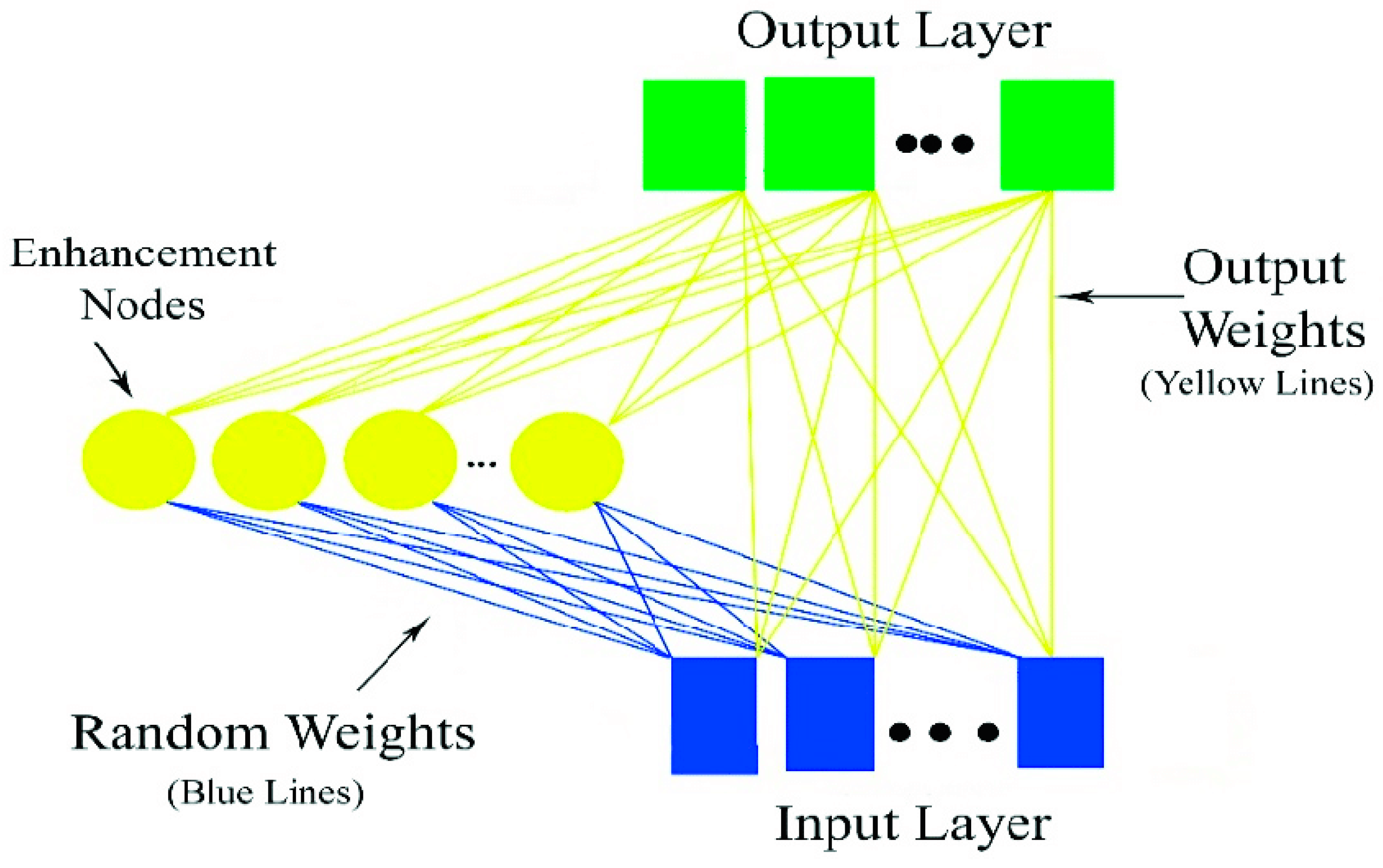
In this study, the authors present a new method for improving the prediction of air temperature by combining a hybrid random vector functional link network (RVFL) with a heuristic optimization technique called Water Cycle-Moth Flame Optimization (WCAMFO). The method is compared to other RVFL-based approaches, such as RVFL-WCA, RVFL-MFO, RVFL-WCAMFO, and single RVFL, in order to evaluate its performance. In Section 2, the authors discuss the most popular machine-learning-based techniques and their related topics. They also present the RVFL model and its implementation with the WCAMFO algorithm, which is designed to improve the accuracy of temperature predictions. In Section 3, the authors present the results and discussion of the comparison of the different methods. They evaluate the performance of the proposed method in terms of prediction accuracy and computational efficiency. Finally, in Section 4, the authors discuss the findings of the study and identify research gaps in temperature forecasting. They conclude that the proposed method, RVFL paired with WCAMFO, is a promising approach for improving the prediction air temperature. They also suggest that further research is needed to further improve the performance of the model and to make it more widely applicable.

2. Case Study

The climate of the study area is subhumid, warm, and subtropical (Figure 1). The western part of Bangladesh encompasses approximately 41%, or 60,165 km2 of the country [33]. The subtropical monsoon climate is experienced by three distinct seasons: winter (Nov–Feb), which is characterized by being cool and dry with almost no rainfall; the premonsoon (Mar–May), characterized by being hot and dry; and the monsoon (Jun–Oct), characterized by heavy rainfall. The annual rainfall over the last 30 years was 1600 mm, less than the national average of 2550 mm in the study area [34]. The annual rainfall and average temperature in the study area range from 1492 to 2766 mm, with an average of 1925 mm, and 24.18 to 26.17 °C, with an average of 25.44 °C, respectively [35]. Two distinct landforms characterize the study region. One is the Barind Tract, dissected and undulating, and the other is the floodplains. Geologically, the area consists of the stream and inter-stream recent and Pleistocene sediments that overlie the Gondwana sediments. In this study, daily and monthly average data of temperature variable for the Rajshahi climatic station is collected from the Bangladesh Meteorological Department (BMD) for the duration of 27 years (1992 to 2018). For data modeling, three equally spaced testing datasets of M1, M2, and M3 using nine years of data.

3. Methods

3.1. Random Vector Functional Link Network (RVFL)

The Random vector functional link (RVFL) network (Figure 2), a modified version of the conventional single-layer feed-forward neural network, was introduced through a successful learning process [36,37]. Input and output layers are connected directly in the RVFL network’s general layout, which also includes a layer of nodes known as enhancement neurons that serves as the network’s hidden layer. The following is a summary of the RVFL network’s fundamental principles:
  • Overfitting problems are avoided and RVFL’s performance is improved because of the layer-by-layer interaction between the input and output layers.
  • With randomly selected input weights that are not subject to modification during the training phase, the computational cost is reduced.
  • Ridge regression [38] or the Moore-Penrose pseudo-inverse are used to produce the output weights, which are adjusted by traditional learning techniques [37].
  • The main advantage of RVFL is that it offers a potential remedy for several critical problems with the conventional learning algorithm in the multi-layer neural network design (poor convergence speed and large computing weight).
  • In order for the RVFL to function, m training samples of data are fed into the network, with each sample denoted by ( 𝓍 𝒾 , 𝓎 𝒾 ), where 𝓍 𝒾 and 𝓎 𝒾 stand for the input and output, respectively. After that, the input is transmitted to the enhancement nodes, and the final result is calculated as follows [39]:
    O 𝒿 ( 𝒶 𝒿 𝓍 𝒾 + β 𝒿 ) = 1 1 + e ( 𝒶 𝒿 𝓍 𝒾 + β 𝒿 ) , β 𝒿 [ 0 , S ] ,   𝒶 𝒿 [ S , S ]
where 𝒶 𝒿 represent the weights of the input layer and enhancement nodes. The bias is denoted by β 𝒿 , while the scale factor is denoted by S . In conclusion, the output of the RVFL network can be stated as follows:
Z = 𝓌
where is a matrix containing the data from 1 input data, and 2 result from the enhancement node
1 = [ 𝓍 11 𝓍 1 𝓃 𝓍 N 1 𝓍 N 𝓃 ] ,     2 = [ O 1 ( 𝒶 1 𝓍 1 + 𝒹 1 ) O 𝒫 ( 𝒶 𝒫 𝓍 1 + β 𝒫 ) O 1 ( 𝒶 1 𝓍 N + 𝒹 1 ) O 𝒫 ( 𝒶 𝒫 𝓍 N + β 𝒫 ) ]
Through the use of the Moore-Penrose pseudo-inverse, the weight 𝓌 can be calculated:
𝓌 = 𝓑†𝒵
where † is the Moore-Penrose pseudo-inverse.

3.2. Moth-Flame Optimization Algorithm (MFO)

The new biologically-inspired optimization method known as the MFO algorithm is based on the flight pattern of a moth, which spirals toward and then clings to an artificial light source to achieve optimization [40]. The essential premise of MFO algorithm (Figure 3) is as follows.
Assume that the matrices = ( N , d i m ) and = ( N , d i m ) are used to represent the set of moth and flame, and that flames and moths are potential solutions to issues. In the formula, N represents the maximum number of flames and d i m represents the population of moths. The flames reflect the best location obtained from the moths, and the moths represent the real search topics travelling through the scope of the search. According to the greedy retention principle, which stipulates that the flame structure preserves the best N solutions to the moth’s flight history, the position of the moth and the flame structure are updated with the moth’s spiral flight [41]. The spiral flying mechanism has the following characteristics:
(1)
The search area must include the spiral flying space.
(2)
The moth serves as the origin of spiral flying.
(3)
The flame position is the spiral’s conclusion.
To update each moth’s location and replicate its flight mode, use Equation (5).
𝒾 = D 𝒾 𝒷 𝓉 c o s ( 2 π 𝓉 ) + 𝒿
𝒾 and 𝒿 in the equation stand for the 𝒾 t h moth and the 𝒿 t h flame, respectively. D 𝒾 is the distance between them, and its expression is given in Equation (6). The spiral 𝒷 flight shape is defined by 𝒷 ( 𝒷 = 1) is the spiral flight coefficient, and Equation (7) shows its 𝓉 expression. Its value range is [−1, 1].
D 𝒾 = | 𝒿 𝒾 |
𝓉 = ( + 1 ) × r a n d + 1
where and stand for the number of iterations’ maximum and current durations. A random number with a uniform rand distribution is called rand. When 𝓉 = −1, it indicates that the distance between the flame and the moth is at its shortest, and when 𝓉 = 1, it indicates that it is at its greatest.
Equation (8) is utilized to minimize the number of flames during each iteration in an adaptive linear way, increasing the moth’s capacity to mine locally in subsequent iterations. At the start of the iteration, there are N flames. The moths only adjust their position around the best flame at the end of iteration, greatly enhancing the search capabilities of the algorithm.
f l a m e n o = r o u n d ( N × N 1 )
Numerous MFO variants have been developed, including Lévy-flight moth-flame optimization (LMFO) [42], non-dominated sorting moth flame optimization (NS-MFO) [43], enhanced moth-flame optimization (EMFO) [44], water cycle-moth-flame optimization (WCMFO) [45], and sine-cosine moth-flame optimization (SMFO) [46]. MFO and its derivatives still have some flaws, such as poor population diversity [47], premature convergence, local optima trapping [48], and an imbalance between exploration and exploitation [49], which prevent them from meeting the needs of the optimization process for difficult problems. The majority of moths are stuck in the local optima in the early iterations, leading to poor population diversity, which is the main cause of these MFOs’ limitations [49].

3.3. Water Cycle Optimization Algorithm (WCA)

Eskandar et al. [50] created the WCA in accordance with the natural water cycle or hydrological cycle. The WCA technique begins with the starting population, referred to as raindrops, like other meta-heuristic algorithms. The initial assumption is that there is rain or other precipitation. The best individual (a water drop) is picked to represent the sea. The remaining raindrops are then regarded as streams that empty into rivers and seas, whereas some of the nice droplets are regarded as rivers. A single solution is referred to as a “raindrop” in the WCA method. Such an array is referred to as a “chromosome” in the GA method. A raindrop is an X N v a r array in a problem of multidimensional optimization, defined as Equation (9).
R a i n d r o p = X 1 , X 2 , X N v a r
where X 1 to X N v a r represent the decision variables. To begin with, a sample of the raindrop matrix with the size of 𝒩pop × 𝒩 var is randomly generated.
P o p u l a t i o n   o f r a i n d r o p s = [ b m a t r i X R a i n d r o p 1 R a i n d r o p 2 ; R a i n d r o p N p o p b m a t r i X ] = [ b m a t r i x X 1 1 X 2 1 X 3 1 X N v a r 1 ; X 1 N p o p X 2 N p o p . . X N v a r N p o p b m a t r i x
where 𝒩pop and 𝒩var are the initial population (number of raindrops) and the variation population, respectively. The values of the provided cost function ( C ) are obtained from Equation (11).
C 𝒾 = C o s t 𝒾 = f ( X 1 𝒾 ,   X 2 𝒾 , , , , , X N v a r 𝒾 ) ,   𝒾 = 1 ,   2 ,   3 , , , N p o p
where C 𝒾 is each drop’s target value. The N S   number of the best droplets is chosen as the sea and river after the 𝒩pop number of raindrops (first stage) is formed. The raindrops that fall in the fewest numbers are referred to as the sea. N S   is the total of the rivers (a parameter that is applied) and the sea (Equation (12)). The remaining population is calculated using Equation (13) and includes streams that may directly flow into rivers or the sea.
N S = N u m b e r o f r i v e r + 1 s e a
N R a i n d r o p = N p o p N S
To identify or assign raindrops to rivers and seas using Equation (14), based on the force of the flow.
N S 𝓃 = r o u n d { | C o s t 𝓃 𝒾 = 1 N S C o s t 𝒾 | × N R a i n d r o p s } ,   𝓃 = 1 , 2 , , , , , N S
where N S 𝓃   is the total number of streams that empty into a given river or body of water. The randomly selected distance and a stream that flows up to the river are used in Equation (15) to establish a connection between them.
X ( 0 ,   C × 𝒹 ) ,   C > 1
Using Equations (16) and (17), updated positions of streams and rivers can be found.
X S t r e a m 𝒾 + 1 = X S t r e a m 𝒾 + r a n d × C × ( X R i v e r 𝒾 X S t r e a m 𝒾 )
X R i v e r 𝒾 + 1 = X R i v e r 𝒾 + r a n d × C × ( X S e a 𝒾 X R i v e r 𝒾 )
where r a n d is a consistent random number between 0 and 1. The location of the river and the stream will change if the stream provides a better solution than the river to which it is connected. Rivers and seas are likewise susceptible to this transformation in the same way. One of the most crucial reasons impeding the algorithm’s speedy convergence and becoming stuck in the local minimum is evaporation. When seawater enters rivers or streams, the evaporation process causes it to evaporate once more. Pseudo-code is used to show how to determine whether a river drains into the sea (Equation (18)).
i f | X S e a 𝒾 X R i v e r 𝒾 |
where 𝒹max is a negligible number (close to zero). As a result, the river has reached the sea if the distance between it and it is smaller than 𝒹max. The evaporation process is impacted in this condition, and precipitation will start once there has been enough evaporation. The search intensity close to the sea is controlled by 𝒹max (optimal solution). Equation (19) reduces the value of max in each step.
𝒹 m a x 𝒾 + 1 = 𝒹 m a x 𝒾 𝒹 m a x 𝒾 m a x i t e r a t i o n
After evaporation is accomplished, rainfall is applied. As rain falls, fresh raindrops form streams in various spots. The updated position of streams can be found using Equation (20).
X S t r e a m n e w = + r a n d × ( U )
where and U stand for the problem’s upper and lower limits, respectively. The best newly created raindrops are thought of as rivers, and the remaining raindrops are thought of as fresh streams feeding the rivers. Equation (21) is applied to improve the computational efficiency and convergence rate of the approach for constrained problems.
X S t r e a m n e w = X S e a + μ × r a n d n ( 1 , N v a r )
where the search area near the sea is represented by the factor. Small values cause the algorithm to search in a narrower area near the water, while large values increase the likelihood of leaving the possible area. Its proper value is set to 0.1 [50].

3.4. Hybrid Water Cycle-Moth-Flame Optimization Algorithm (WCAMFO)

Theoretically, the WCA and MFO algorithms showed that the water cycle (WCA) performed admirably throughout the discovery phase but poorly during operator-performed exploitation. As an alternative, the MFO exploited the space very well by using its spiral movement capability, although they frequently remained inherently unable to explore the solution space and was trapped in local optima [45,51]. As a result, by combining the benefits of the two methods, a hybrid algorithm can be a good alternative and help to further improve the optimization problem. Two of the major benefits of merging the WCA and the MFO, according to Khalil pourazari and Khalil pourazary [45] are that: the initial improvement was that the position in the WCA was updated using the spiral movement of the moths. The second enhancement is to improve the precipitation process. The so-called “Levy flight”, from a mathematical perspective, allows the streams to arrange themselves better:
X 𝒾 + 1 = X 𝒾 + L e v y ( d i m ) X 𝒾

3.5. Performance Evaluation

Four statistical indicators of root mean squared error (RMSE), mean absolute error (MAE), determination coefficient (R2) and Nash efficiency (NSE) were utilized for performance examination of RVFL, RVFL-WCA, RVFL-MFO, and RVFL-WCAMFO models for modeling air temperature. RMSE, MAE, NSE and R2 can be expressed, respectively, by:
R M S E = 1 N 𝒾 = 1 N [ ( T c ) 𝒾 ( T p ) 𝒾 ] 2
M A E = 1 N 𝒾 = 1 N | ( T c ) 𝒾 ( T p ) 𝒾 |
N S E = 1 𝒾 = 1 N [ ( T c ) 𝒾 ( T p ) 𝒾 ] 2 𝒾 = 1 N [ ( T c ) 𝒾 ( T c ) ¯ ] 2
R 2 = 𝒾 = 1 N [ ( ( T c ) 𝒾 ( T c ) ¯ ) ( ( T p ) 𝒾 ( T p ) ] ¯ 𝒾 = 1 N [ ( T p ) 𝒾 ( T p ¯ ) ] 2 𝒾 = 1 N [ ( T c ) 𝒾 ( T c ¯ ) ] 2
where T c , T p , T c ¯ and T p ¯ indicate calculated, predicted, mean calculated, and mean predicted air temperature, respectively, and N is the quantity of data.

4. Results and Discussion

In this section, the single optimization techniques (RVFL, WCA, MFO, WCAMFO, and all combinations) for modeling air temperature were technically discussed and comparatively analyzed. Prior to the computational schema, eight different input combinations were proposed for the development of each algorithm (M1, M2, and M3) (Table 1). M1, M2, and M3 testing datasets were formed on the basis of cross-validation technique. According to this technique, the whole dataset is divided into three equal parts and all three testing datasets are formed using equally 1/3 ratio of the whole dataset, whereas during analyzing one testing dataset, the remaining 2/3 of the whole dataset is used as a training dataset. It is worth noting that selecting input combinations for building machine learning is paramount and has been recommended in several works of literature [52,53,54]. Subsequently, the predictive models were assessed by four statistical matrices, including NSE, MAE, RMSE, and R2. For modeling nonlinear environmental variables such as air temperature, it is always recommended to employ several performance indicators to comprehend the stochastic influence of air temperature estimation based on the global and regional scale of climate change impact. According to Benaafi et al., [55] evaluation criteria should involve at least one error-of-fit (e.g., MAE) and one goodness-of-fit (e.g., NSE) for any reliable analysis.
Furthermore, another essential part in AI-based models that receives less attention is controlling the hyper-tuning parameters in the modeling process. The parameters’ optimization setting of each algorithm as tabulated in Table 2 were used for attaining the training and validation phase of each model’s combination. The external configuration and the un-estimated parameters from each model are referred to as hyper parameter.
These parameters were tuned to determine the best values to solve a certain predictive model. It should be noted that different approaches were used for the determination of the best tuning parameters to find the most skillful predictions, for example, trial and error, rules of thumb, etc. Despite less attention than was previously observed in modeling the monthly and daily air temperature using machine learning, this study was the first work to employ the above-mentioned techniques to model air temperature to the best of the authors’ knowledge.

4.1. Results for Monthly Air Temperature Modeling

The predictive outcomes in terms of several performance indicators for the RVFL monthly scale approach are presented in Table 3. The results indicated that M1 (viii) with the input combination of (best p, best T) attained the maximum values of goodness-of-fit of R2 = 0.921, NSE = 0.92, and minimum values of RMSE = 1.450, MAE = 1.203 in comparison with M2 and M3 combinations. Furthermore, the best predictive combination of M2 and M3 were found to be M2 (viii), and M3 (viii), respectively. The outcomes of the model RVFL for the monthly time scale depicted that model combination (viii) with (best p, best T) emerging as the most reliable input with the highest accuracy in the testing phase. The fitting comparison of models shows that the best models M1 (viii) increased the predictive skills with giving range between 3% to 37% of the rest combination (i, ii, iii, iv, and vii), M2 (viii) within 4% to 42%, and lastly M3 (vii) within the range of 1% to 42%. The overall comparison of all the three models indicated that M1 (viii) with the smallest absolute error proved merit than the other models. This can be justified by considering the mean values in Table 3. In addition, 
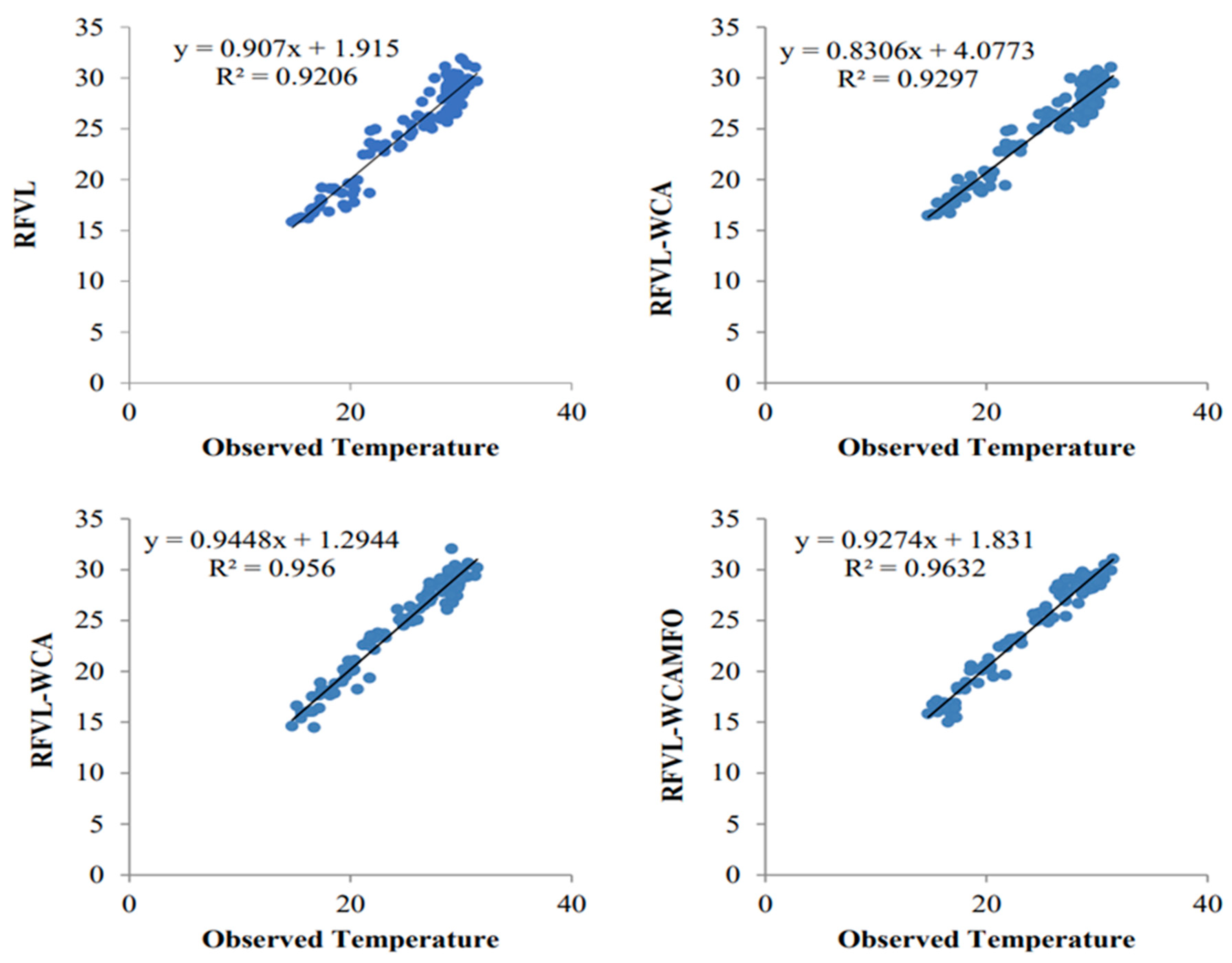
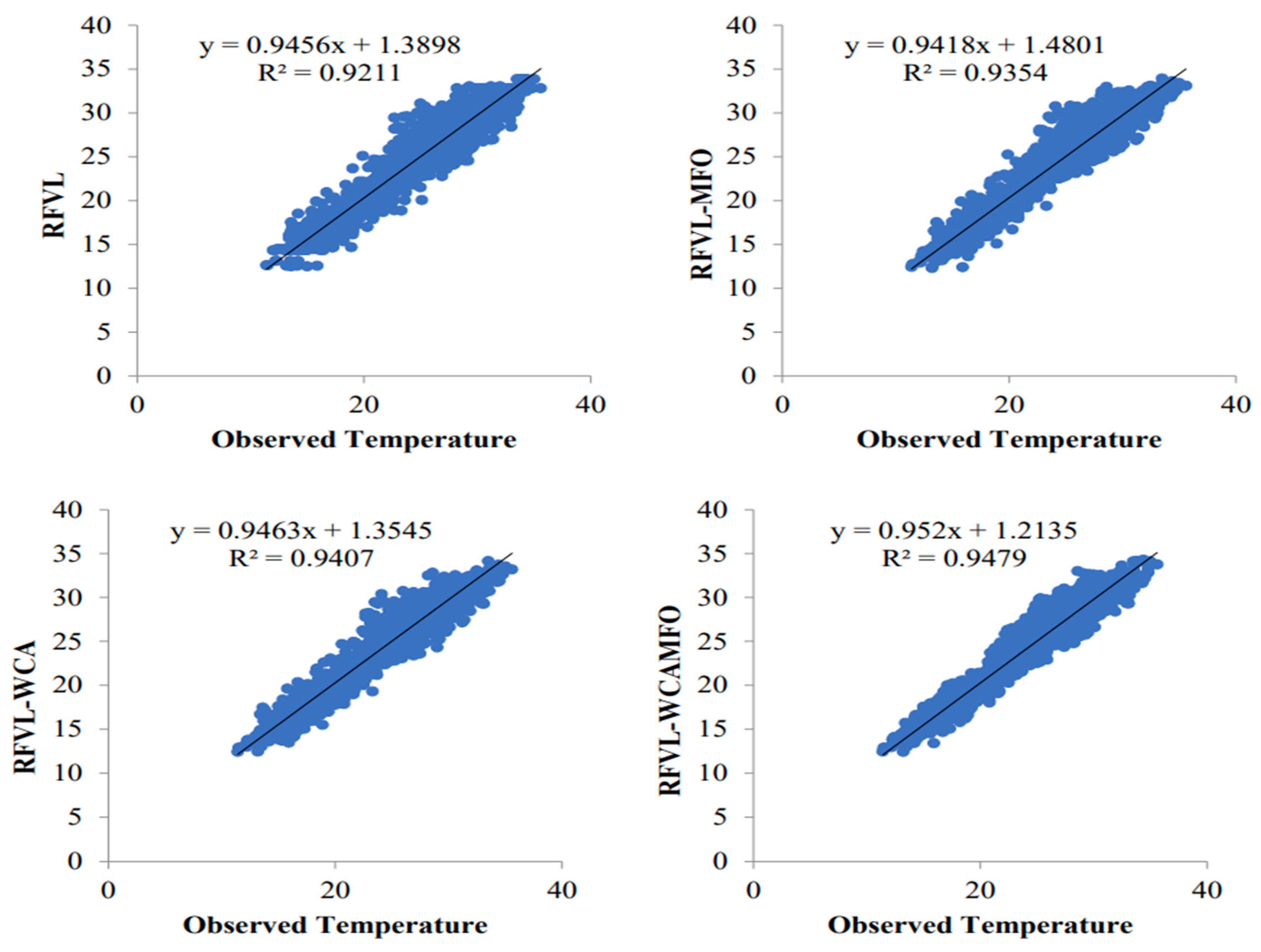
Figure 4 shows the scatterplots of the observed and predicted temperature by different RVFL-based models in the test period using the best input combination for a monthly time scale.
In addition to the application of RVFL models, the hybrid optimization models using RVFL-WCA, RVFL-MFO, and RVFL-WCAMFO for monthly air temperature modeling were employed in this study and the estimated outcomes were generated in Table 4, Table 5 and Table 6.
The concept of coupling RVFL with three different optimization algorithms was attributed to its universal approximation ability and fast training speed as reported by several literatures. Hence, during the monthly air temperature modeling using RVFL-WCA, the M1 (viii) with parameters combination (Tt-1, Tt-2, Tt-3) in Table 4 supported the best against all the combination (M1, and M2). The quantitative comparison of the best outcomes with regards to absolute error of the M1, M2, and M3 demonstrated that M1 (viii) reduced the prediction error by approximately 12% and 6% for M2, and M3, respectively. This outcomes was in line with the work conducted by Smith et al., [56] that improved the estimation accuracy of air temperature using ANN models and obtained the hourly prediction accuracy more than 90% in terms of fitting of the models (see Figure 5). The major difference between our work and that of Smith et al. [56] is the employment of recently developed state-of-the-art models supported by optimization algorithms that provide desirable results with fewer input combinations. The overall results can also be depicted using violin plots as presented in
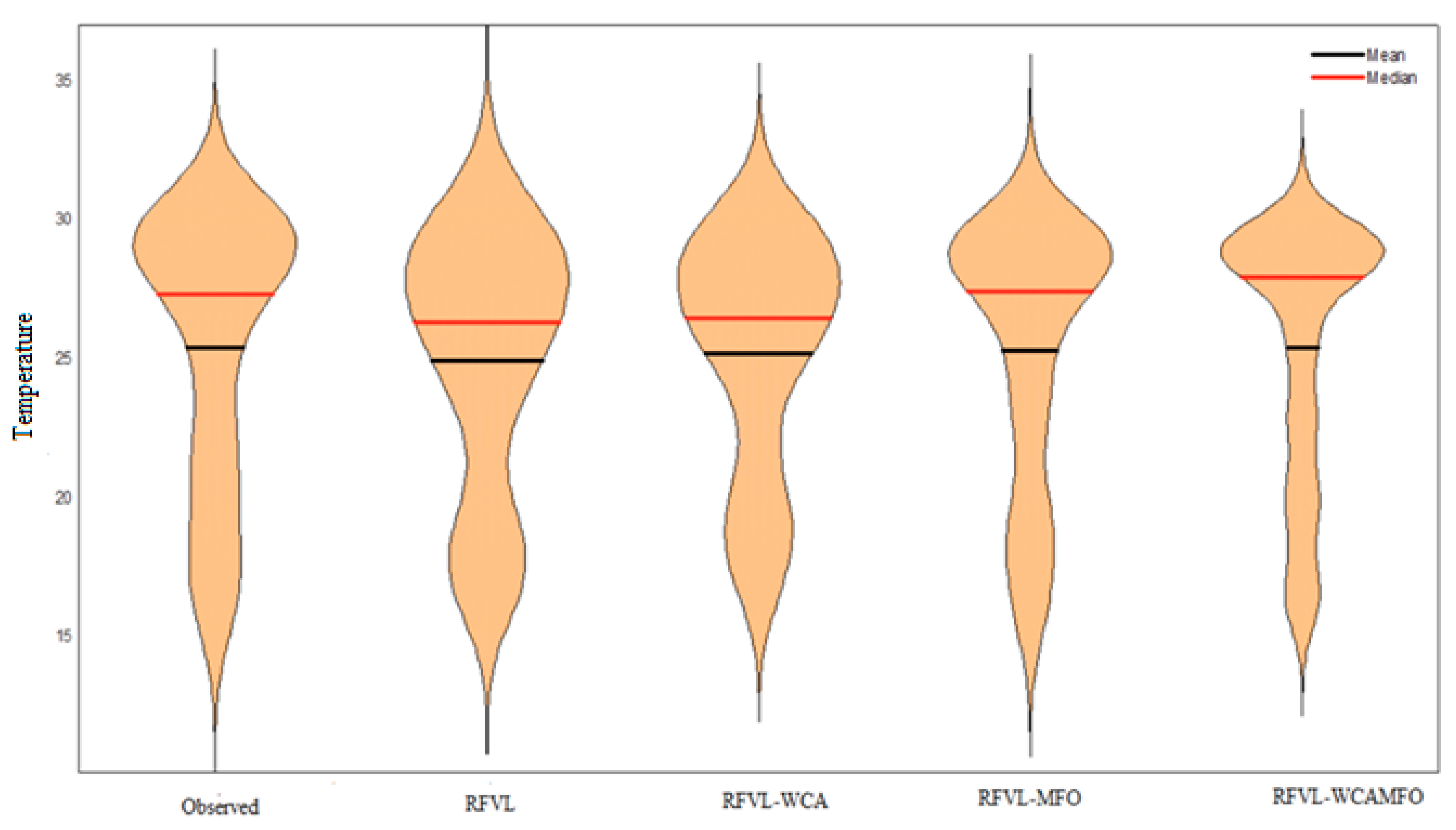
 Figure 6.
Based on the present outcomes, it is worth mentioning that computational approaches play an essential role in handling any type of chaotic pattern. The inputs and response variables justified merit with reasonable accuracy using our established models. To give credit and compare our established outcomes, this study was compared with the selected state-of-the-art models for examples [57,58,59,60,61,62,63] in terms of the popularity of the ML model and proved satisfactory. Other MLS models could be simulated similarly using the same problems.

4.2. Results for Daily Air Temperature Modeling

In this section, the daily air temperature was also simulated at study locations. Note that the combination of modeling the short and long extreme weather changes for air temperature, for example, daily and monthly modeling received less, or no attention based on the authors’ knowledge, despite other hydrological time series processes such as rainfall and run-off already reporting similar scenarios [57,58]. Air temperature modeling and prediction of air pollution serves as major environmental monitoring in different regions. This study is devoted to demonstrating daily and monthly information to come up with satisfactory estimation methodologies for the decision-maker and concern authorities with regards to short- and long-term environmental sustainability. The simulated results for a daily time scale of air temperature for RVFL, RVFL-WCA, RVFL-MFO, and RVFL-WCAMFO are presented in Table 7, Table 8, Table 9, and Table 10, respectively. The results of the daily time scale of air temperature in Figure 7 demonstrated that the first four combinations produce poor to marginal accuracy by comparing the evaluation matrices (MAE, NSE, R2, and RMSE). However, during the daily scale, the models with the combination M1-M3 (vii) displayed high accuracy against all the combinations. For example the assessment matrices, the best model, demonstrated that M1 (vii) = MAE (0.947), NSE (0.920), M2 (vii) = MAE (0.988), NSE (0.918), and M3 (vii) = MAE (0.960), NSE (0.92) for air temperature modeling. The detailed results for all the combinations are presented in terms of performance evaluation criteria in Table 7. It can be observed that single standalone models, i.e., RVFL, could produce reasonable accuracy for modeling air temperature. The feasibility of the hybrid state-of-the-art models for modeling air temperature were also presented using the hybrid optimization approach. Furthermore, other different AI models could also be used in the same manner for proper tuning of air temperature prediction. Table 8 demonstrates the results of the model RVFL-WCA for a daily time scale.
It is worth mentioning that optimization algorithms were reported generally to optimize the tuning parameters and enhance the predictability of the models [59,60]. This was justified in the presented study where the combination (vii) became the most reliable among the other seven combinations. The numerical outcomes of RVFL-WCA for a daily time scale show that M1(vii) = RMSE (1.218), R2 (0.936), M2(vii) = RMSE (1.227), R2 (0.937), and M3 (vii) = RMSE (1.261), R2 (0.927). The capability of daily air temperature modeling is presented graphically in the scatter plot (Figure 7). The scatter plots of the observed and predicted air temperature by different RVFL-based models in the test period using the best input combination for a monthly time scale indicated that RVFL-WCAMFO attained the highest accuracy of more than 94.8% against the other, which have the accuracy ranging from 92–94%.
Similarly, the output of Table 9 for the results of the model RVFL-MFO for daily time scale indicated that M1 (vii) = MAE (0.930), NSE (0.937), M2 (vii) = MAE (0.926), NSE (0.939), M3(vii) = MAE (0.940), NSE (0.932).
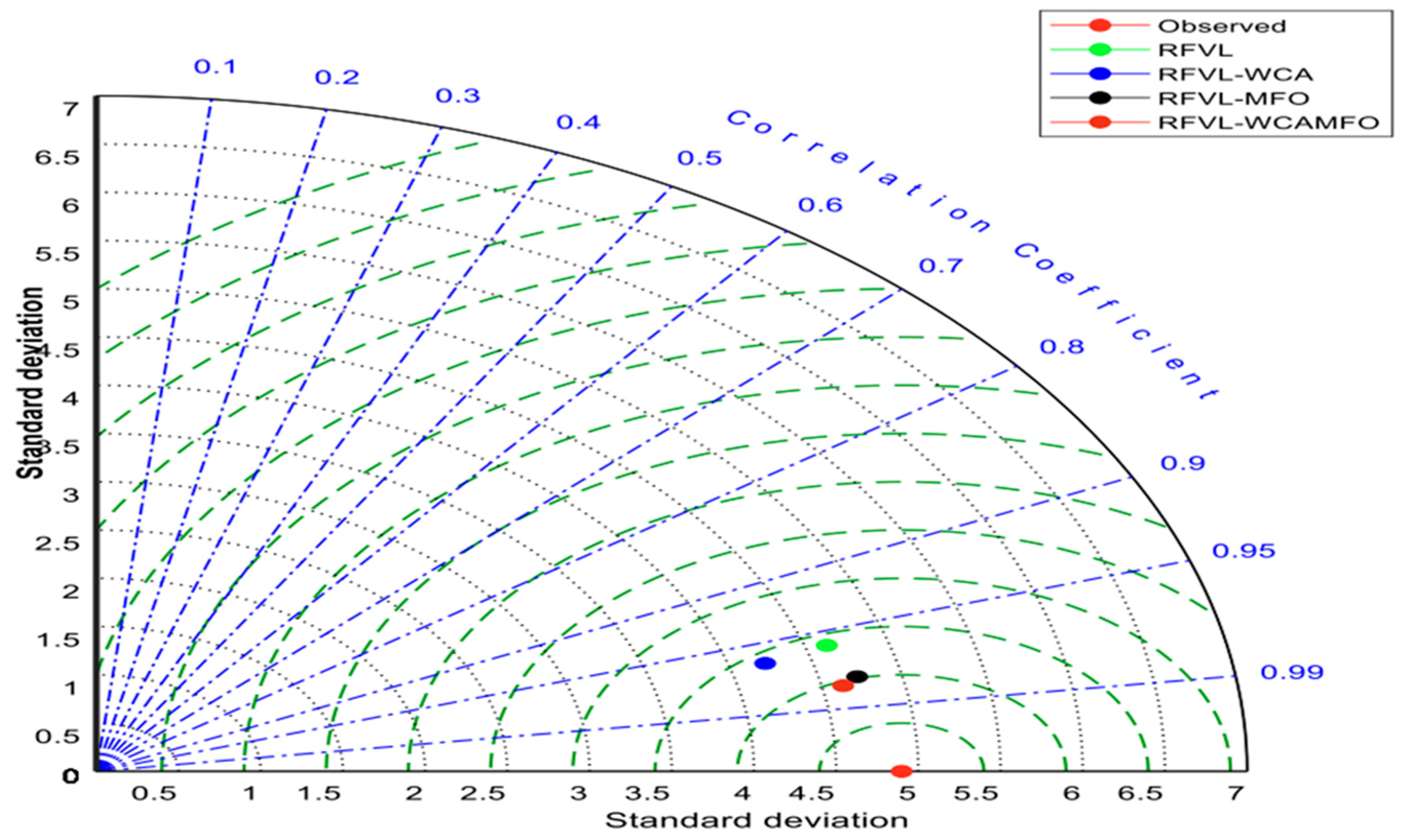
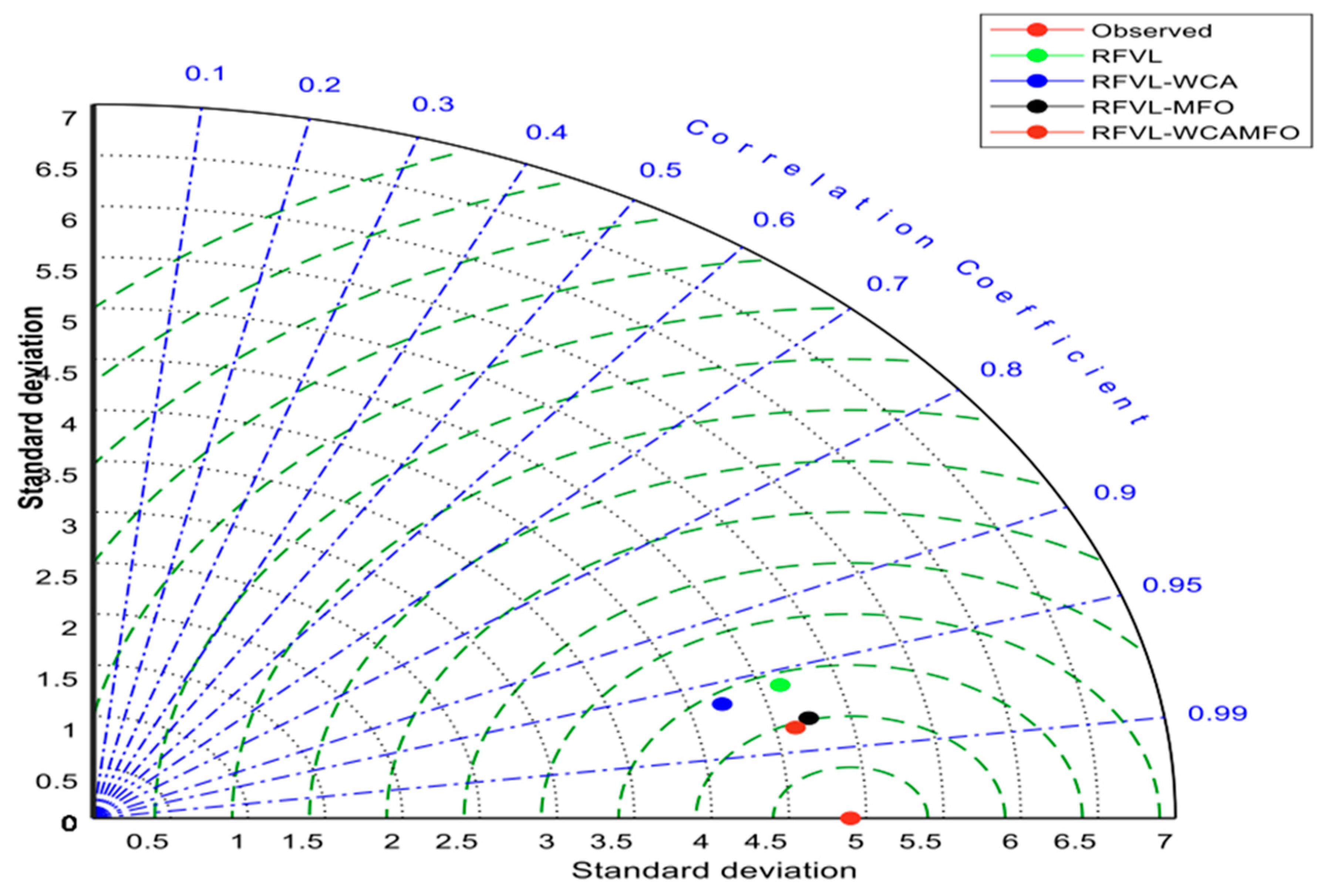
For computational modeling of air temperature, it is obvious that step-ahead combination of temperature produces the best outcomes; this is in line with the presented study where the combination M1-M3 (vii) Tt-1, Tt-2, Tt-3 produced the best predictive skills. The obtained modeling architecture justified that minimum input parameters based on the accurate feature selection could lead to more improved prediction results than large combination. Similarly, the results show that all combinations with precipitation as inputs were less accurate, whereas temperature combination as previous inputs provided more accurate results. The predicted results of daily air temperature can also be visualized in the Taylor diagram using different matrices, as shown in Figure 8. The major advantage of the Taylor diagram is centered towards understanding the concept of correlation, standard deviation, and RMSE.
It can also be proved in this study demonstration that precipitation inputs have less effect on temperature, whereas what we see in literature, temperature inputs have good affect in modeling runoff and rainfall, for example, [61,62,63,64]. These results also demonstrated the necessity and importance of accurate temperature modeling as extreme rainfall events such as typhoon, cloud bursting, heat wave, and extreme runoff events such as drought and flood can be avoided if we can model air temperature precisely because this input has a very good affecting relationship with precipitation and runoff. It is a well-known fact that remarkable progress has been recorded in temperature modeling, but still some limitations exist, especially with a traditional theoretical approach. Table 10 presents the results of the model RVFL-WCAMFO for a daily time scale.
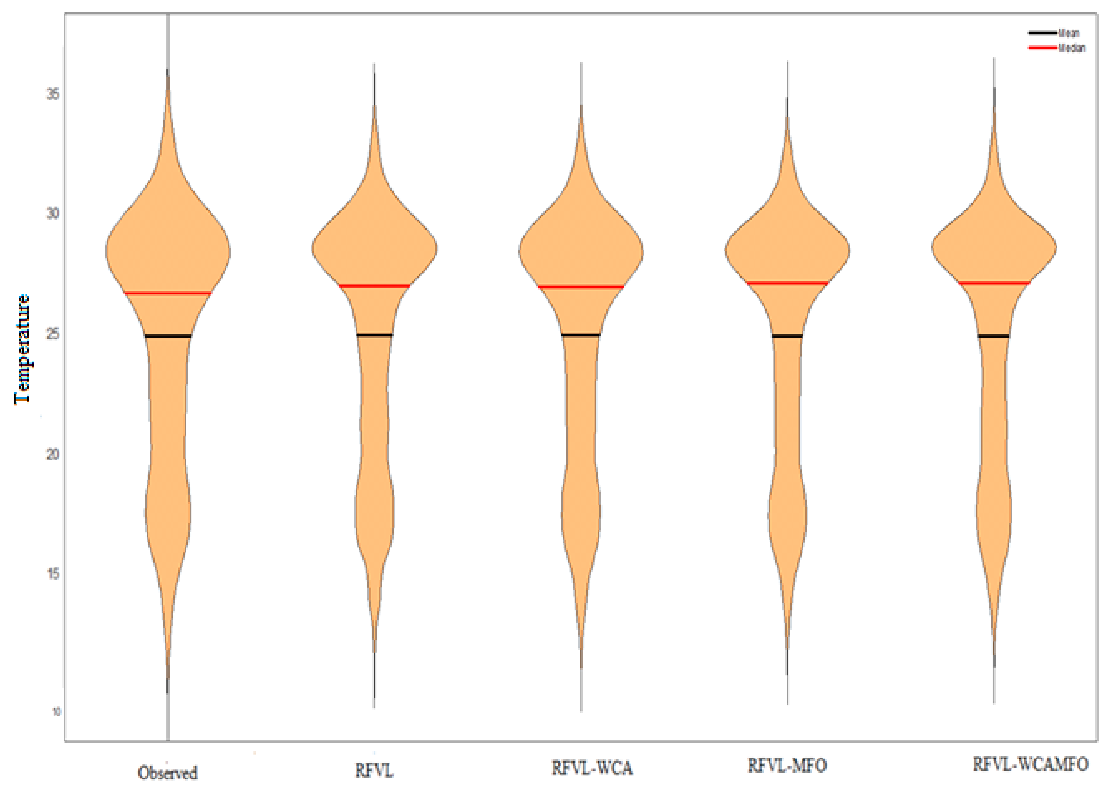
From the results it can be observed that the best models are still a temperature-related combination (vii). The summary of the numerical results for the best models demostrated that M1(vii) = RMSE (1.218), MAE(0.921), NSE(0.947), R2(0.948), M2 (vii) = RMSE (1.204), MAE (0.911), NSE (0.940), R2 (0.945), and M3 (vii) = RMSE (1.244), MAE (0.931), NSE (0.937), R2 (0.939). Addition visualization based on the predicted results is presented in Figure 9.

5. Conclusions

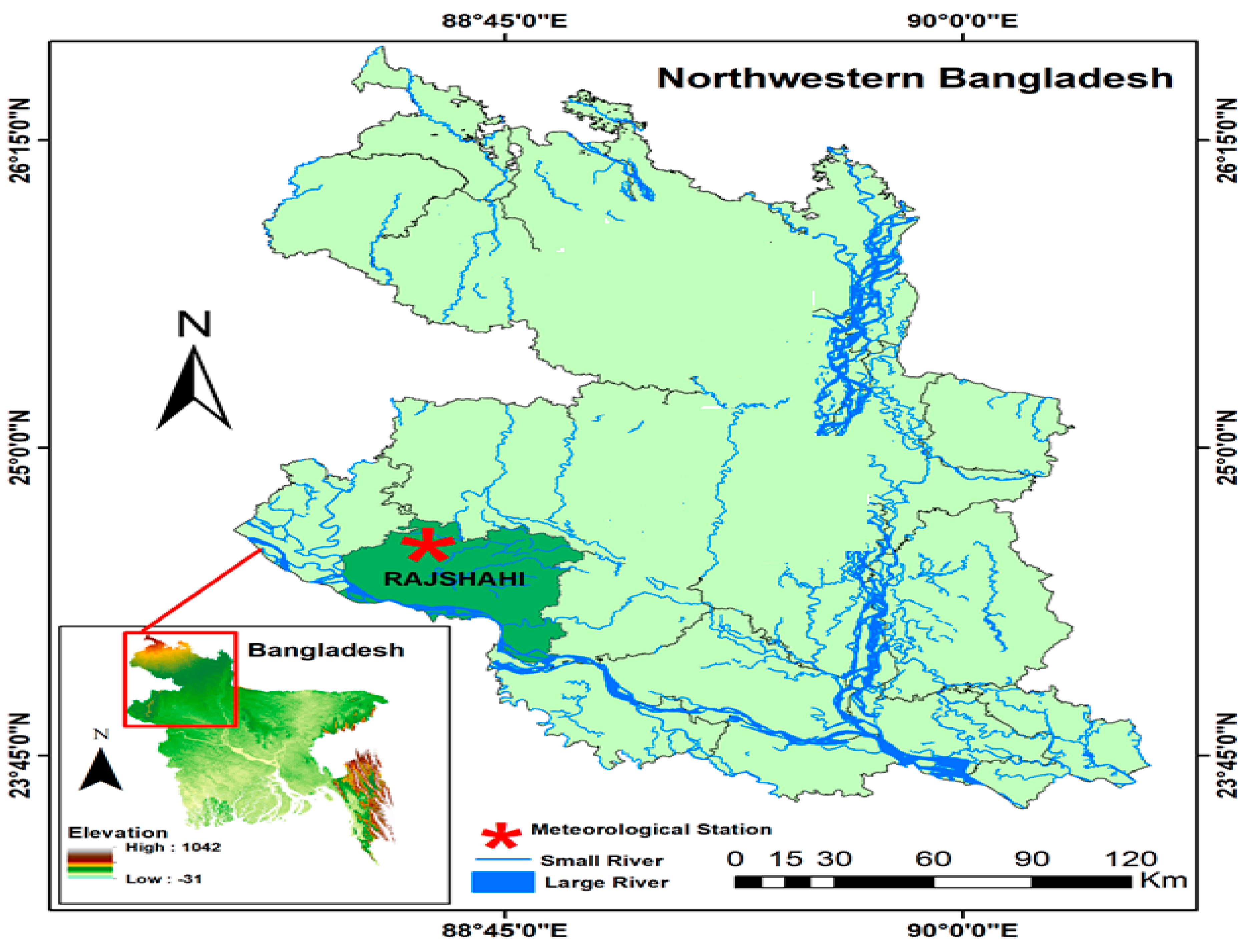
The prediction accuracy of RVFL with three hybrid metaheuristic models, namely RVFL-WCA, RVFL-MFO, and RVFL-WCAMFO, for predicting the air temperature of the Rajshahi station of western Bangladesh was assessed in this paper. The standalone RVFL and three metaheuristic models were examined using three algorithms, including M1, M2, and M3, with eight different input combinations with the help of RMSE, MAE, and R2 performance evaluation indexes, including scatter plots, and Taylor and violin charts. The metaheuristic algorithms made the single RFVL more accurate when it was used to simulate (in the training stage) and predict (in the testing stage) the monthly air temperature based on M1, M2, and M3. The monthly air temperature modeling using a standalone RVFL model showed that the best model, M1 (viii), increased the predictive skills by giving variations from 3% to 37% of the remaining combinations (i, ii, iii, iv, and vii), M2 (viii) within 4% to 42%, and lastly, M3 (vii) within the range of 1% to 42%. The monthly air temperature modeling using hybrid optimization RVFL-WCA revealed that the M1 (viii) with parameter combinations (Tt-1, Tt-2, Tt-3) indicated the best against all the combinations (M1 and M2). The RMSE of the M1, M2, and M3 demonstrated that M1 (viii) reduced the prediction error by approximately 12% and 6% for M2 and M3, respectively, for the monthly time scale. During the daily scale, the RVFL-WCAMFO models with the combination (vii) displayed high accuracy against all the combinations for air temperature modeling. They have attained more than 94.8% accuracy against the other three models, with an accuracy range of 92–94%, though single standalone models, i.e., RVFL, could produce reasonable accuracy for modeling air temperature. The precision comparison of the algorithms exposed that the precision positions were in descending order: RVFL-WCAMFO > RVFL-WCA > RVFL-MFO in forecasting air temperature. According to the outcomes of this research, the use of hybrid metaheuristic i.e., RFVL-WCAMFO is suggested for air temperature prediction. Thus, the suggested model can be helpful for policymakers in alleviating the effects of temperature and recommending effective plans for agricultural crop production. The key limitation of this research was the use of input data from just one station in western Bangladesh to examine the accuracy of the models. In future studies, these models can be evaluated using more datasets from different regions. These suggested advanced hybrid models also can be evaluated with other different hybrid machine learning models in the future studies.

Author Contributions

Conceptualization: R.M.A., S.G.M., F.A. and Z.C.; formal analysis: R.R.M. and A.R.M.T.I.; validation: R.M.A., F.A., Z.C., S.G.M. and A.R.M.T.I.; supervision: A.R.M.T.I. and Z.C.; writing—original draft: R.M.A., S.I.A., R.R.M., S.G.M., Z.C., F.A. and A.R.M.T.I.; visualization: R.M.A. and S.I.A.; investigation: S.I.A., R.R.M. and F.A. All authors have read and agreed to the published version of the manuscript.

Funding

This research received no external funding.

Institutional Review Board Statement

Not applicable.

Informed Consent Statement

Not applicable.

Data Availability Statement

The data presented in this study will be available on an interesting request from the corresponding author.

Conflicts of Interest

There is no conflict of interest in this study.

References

  1. Allan, R.P.; Hawkins, E.; Bellouin, N.; Collins, B. Summary for Policymakers; IPCC: Geneva, Switzerland, 2021. [Google Scholar]
  2. Nita, I.A.; Sfîcă, L.; Voiculescu, M.; Birsan, M.V.; Micheu, M.M. Changes in the global mean air temperature over land since 1980. Atmos. Res. 2022, 279, 106392. [Google Scholar] [CrossRef]
  3. Alvi, U.; Suomi, J.; Käyhkö, J. A cost-effective method for producing spatially continuous high-resolution air temperature information in urban environments. Urban Clim. 2022, 42, 101123. [Google Scholar] [CrossRef]
  4. Yu, M.; Xu, F.; Hu, W.; Sun, J.; Cervone, G. Using Long Short-Term Memory (LSTM) and Internet of Things (IoT) for localized surface temperature forecasting in an urban environment. IEEE Access 2021, 9, 137406–137418. [Google Scholar] [CrossRef]
  5. Cho, H.J.; Cheon, S.Y.; Jeong, J.W. Preliminary study on air-to-air latent heat exchanger fabricated using hollow fiber composite membrane for air-conditioning applications. Energy Convers. Manag. 2022, 251, 115000. [Google Scholar] [CrossRef]
  6. Lembrechts, J.J.; Hoogen, J.V.D.; Aalto, J.; Ashcroft, M.B.; De Frenne, P.; Kemppinen, J.; Kopecký, M.; Luoto, M.; Maclean, I.M.D.; Crowther, T.W.; et al. Global maps of soil temperature. Glob. Change Biol. 2022, 28, 3110–3144. [Google Scholar] [CrossRef]
  7. Di Blasi, C.; Renzi, M.; Michelozzi, P.; Donato, F.D.; Scortichini, M.; Davoli, M.; Forastiere, F.; Mannucci, P.M.; Stafoggia, M. Association between air temperature, air pollution and hospital admissions for pulmonary embolism and venous thrombosis in Italy. Eur. J. Intern. Med. 2022, 96, 74–80. [Google Scholar] [CrossRef]
  8. Demissie, T.A.; Sime, C.H. Assessment of the performance of CORDEX regional climate models in simulating rainfall and air temperature over southwest Ethiopia. Heliyon 2021, 7, e07791. [Google Scholar] [CrossRef]
  9. Yuan, X.; Chen, C.; Lei, X.; Yuan, Y.; Muhammad Adnan, R. Monthly runoff forecasting based on LSTM–ALO model. Stoch. Environ. Res. Risk Assess. 2018, 32, 2199–2212. [Google Scholar] [CrossRef]
  10. He, Y.; Chen, C.; Li, B.; Zhang, Z. Prediction of near-surface air temperature in glacier regions using ERA5 data and the random forest regression method. Remote Sens.Appl. Soc. Environ. 2022, 28, 100824. [Google Scholar]
  11. Xiu, Y.; Wang, Q.; Li, Z.; Li, G.; Lu, P. Estimating spatial distributions of design air temperatures for ships and offshore structures in the Arctic Ocean. Polar Sci. 2022, 34, 100875. [Google Scholar] [CrossRef]
  12. Ji, L.; Wang, Z.; Chen, M.; Fan, S.; Wang, Y.; Shen, Z. How much can AI techniques improve surface air temperature forecast?—A report from AI Challenger 2018 Global Weather Forecast Contest. J. Meteorol. Res. 2019, 33, 989–992. [Google Scholar] [CrossRef]
  13. Cifuentes, J.; Marulanda, G.; Bello, A.; Reneses, J. Air temperature forecasting using machine learning techniques: A review. Energies 2020, 13, 4215. [Google Scholar] [CrossRef]
  14. Mohammadi, B.; Mehdizadeh, S.; Ahmadi, F.; Lien, N.T.T.; Pham, Q.B. Developing hybrid time series and artificial intelligence models for estimating air temperatures. Stoch. Environ. Res. Risk Assess. 2021, 35, 1189–1204. [Google Scholar] [CrossRef]
  15. Bayatvarkeshi, M.; Bhagat, S.K.; Mohammadi, K.; Kisi, O.; Farahani, M.; Hasani, A.; Deo, R.; Yaseen, Z.M. Modeling soil temperature using air temperature features in diverse climatic conditions with complementary machine learning models. Comput. Electron. Agric. 2021, 185, 106158. [Google Scholar] [CrossRef]
  16. Ghadiri, M.; Marjani, A.; Mohammadinia, S.; Shirazian, S. An insight into the estimation of relative humidity of air using artificial intelligence schemes. Environ. Dev. Sustain. 2021, 23, 10194–10222. [Google Scholar] [CrossRef]
  17. Meliho, M.; Khattabi, A.; Zejli, D.; Orlando, C.A.; Dansou, C.E. Artificial intelligence and remote sensing for spatial prediction of daily air temperature: Case study of Souss watershed of Morocco. Geo-Spat. Inf. Sci. 2022, 25, 244–258. [Google Scholar] [CrossRef]
  18. Miyano, T.; Girosi, F. Forecasting Global Temperature Variations by Neural Networks; Technical Report; Massachusetts Institute of Technology, Cambridge Artificial Intelligence Laboratory: Cambridge, MA, USA, 1994. [Google Scholar]
  19. Lanza, P.A.G.; Cosme, J.M.Z. A short-term temperature forecaster based on a state space neural network. Eng. Appl. Artif. Intell. 2002, 15, 459–464. [Google Scholar] [CrossRef]
  20. Ustaoglu, B.; Cigizoglu, H.K.; Karaca, M. Forecast of daily mean, maximum and minimum temperature time series by three artificial neural network methods. Meteorol. Appl. A J. Forecast. Pract. Appl. Train. Tech. Model. 2008, 15, 431–445. [Google Scholar] [CrossRef]
  21. Adnan, R.M.; Mostafa, R.R.; Islam, A.R.M.T.; Gorgij, A.D.; Kuriqi, A.; Kisi, O. Improving Drought Modeling Using Hybrid Random Vector Functional Link Methods. Water 2021, 13, 3379. [Google Scholar] [CrossRef]
  22. Abhishek, K.; Singh, M.P.; Ghosh, S.; Anand, A. Weather forecasting model using artificial neural network. Procedia Technol. 2012, 4, 311–318. [Google Scholar] [CrossRef] [Green Version]
  23. Jallal, M.A.; Chabaa, S.; El Yassini, A.; Zeroual, A.; Ibnyaich, S. Air temperature forecasting using artificial neural networks with delayed exogenous input. In Proceedings of the 2019 International Conference on Wireless Technologies, Embedded and Intelligent Systems (Wits), Fez, Morocco, 3–4 April 2019; pp. 1–6. [Google Scholar]
  24. Tran, T.; Bateni, S.; Ki, S.; Vosoughifar, H. A review of neural networks for air temperature forecasting. Water 2021, 13, 1294. [Google Scholar] [CrossRef]
  25. Paniagua-Tineo, A.; Salcedo-Sanz, S.; Casanova-Mateo, C.; Ortiz-García, E.G.; Cony, M.A.; Hernández-Martín, E. Prediction of daily maximum temperature using a support vector regression algorithm. Renew. Energy 2011, 36, 3054–3060. [Google Scholar] [CrossRef]
  26. Ortiz-García, E.G.; Salcedo-Sanz, S.; Casanova-Mateo, C.; Paniagua-Tineo, A.; Portilla-Figueras, J.A. Accurate local very short-term temperature prediction based on synoptic situation Support Vector Regression banks. Atmos. Res. 2012, 107, 1–8. [Google Scholar] [CrossRef]
  27. Mellit, A.; Pavan, A.M.; Benghanem, M. Least squares support vector machine for short-term prediction of meteorological time series. Theor. Appl. Climatol. 2013, 111, 297–307. [Google Scholar] [CrossRef]
  28. Ikram, R.M.A.; Mostafa, R.R.; Chen, Z.; Islam, A.R.M.T.; Kisi, O.; Kuriqi, A.; Zounemat-Kermani, M. Advanced Hybrid Metaheuristic Machine Learning Models Application for Reference Crop Evapotranspiration Prediction. Agronomy 2023, 13, 98. [Google Scholar] [CrossRef]
  29. Chevalier, R.F.; Hoogenboom, G.; McClendon, R.W.; Paz, J.A. Support vector regression with reduced training sets for air temperature prediction: A comparison with artificial neural networks. Neural Comput. Appl. 2011, 20, 151–159. [Google Scholar] [CrossRef]
  30. Salcedo-Sanz, S.; Deo, R.C.; Carro-Calvo, L.; Saavedra-Moreno, B. Monthly prediction of air temperature in Australia and New Zealand with machine learning algorithms. Theor. Appl. Climatol. 2016, 125, 13–25. [Google Scholar] [CrossRef]
  31. Venkadesh, S.; Hoogenboom, G.; Potter, W.; McClendon, R. A genetic algorithm to refine input data selection for air temperature prediction using artificial neural networks. Appl. Soft Comput. 2013, 13, 2253–2260. [Google Scholar] [CrossRef]
  32. Azad, A.; Kashi, H.; Farzin, S.; Singh, V.P.; Kisi, O.; Karami, H.; Sanikhani, H. Novel approaches for air temperature prediction: A comparison of four hybrid evolutionary fuzzy models. Meteorol. Appl. 2020, 27, e1817. [Google Scholar] [CrossRef] [Green Version]
  33. Mallick, J.; Islam, A.R.M.T.; Ghose, B.; Islam, H.T.; Rana, Y.; Hu, Z.; Bhat, S.A.; Pal, S.C.; Ismail, Z.B. Spatiotemporal trends of temperature extremes in Bangladesh under changing climate using multi-statistical techniques. Theor. Appl. Climatol. 2022, 147, 307–324. [Google Scholar] [CrossRef]
  34. Jahan, C.S.; Mazumder, Q.H.; Islam, A.T.M.M.; Adham, M.I. Impact of irrigation in Barind area, NW Bangladesh—An evaluation based on the meteorological parameters and fluctuation trend in groundwater table. J. Geol. Soc. India 2010, 76, 134–142. [Google Scholar] [CrossRef]
  35. Kamruzzaman, M.; Rahman, A.T.M.S.; Kabir, M.E.; Jahan, C.S.; Mazumder, Q.H.; Rahman, M.S. Spatio-temporal analysis of climatic variables in the western part of Bangladesh. Environ. Dev. Sustain. 2016, 18, 89–108. [Google Scholar] [CrossRef]
  36. Mostafa, R.R.; Kisi, O.; Adnan, R.M.; Sadeghifar, T.; Kuriqi, A. Modeling Potential Evapotranspiration by Improved Machine Learning Methods Using Limited Climatic Data. Water 2023, 15, 486. [Google Scholar] [CrossRef]
  37. Pao, Y.H.; Takefuji, Y. Functional-link net computing: Theory, system architecture, and functionalities. IEEE Comput. 1992, 25, 76–79. [Google Scholar] [CrossRef]
  38. Husmeier, D. Random vector functional link (RVFL) networks. In Neural Networks for Conditional Probability Estimation; Springer: London, UK, 1999; pp. 87–97. [Google Scholar]
  39. Elsheikh, A.H.; Shehabeldeen, T.A.; Zhou, J.; Showaib, E.; Abd Elaziz, M. Prediction of laser cutting parameters for polymethylmethacrylate sheets using random vector functional link network integrated with equilibrium optimizer. J. Intell. Manuf. 2021, 32, 1377–1388. [Google Scholar] [CrossRef]
  40. Mirjalili, S. Moth-flame optimization algorithm: A novel nature-inspired heuristic paradigm. Knowl. -Based Syst. 2015, 89, 228–249. [Google Scholar] [CrossRef]
  41. Taher, M.A.; Kamel, S.; Jurado, F.; Ebeed, M. An improved moth-flame optimization algorithm for solving optimal power flow problem. Int. Trans. Electr. Energy Syst. 2019, 29, e2743. [Google Scholar] [CrossRef]
  42. Li, Z.; Zhou, Y.; Zhang, S.; Song, J. Lévy-flight moth-flame algorithm for function optimization and engineering design problems. Math. Probl. Eng. 2016, 2016, 1423930. [Google Scholar] [CrossRef] [Green Version]
  43. Savsani, V.; Tawhid, M.A. Non-dominated sorting moth flame optimization (NS-MFO) for multi-objective problems. Eng. Appl. Artif. Intell. 2017, 63, 20–32. [Google Scholar] [CrossRef]
  44. Xu, L.; Li, Y.; Li, K.; Beng, G.H.; Jiang, Z.; Wang, C.; Liu, N. Enhanced moth-flame optimization based on cultural learning and Gaussian mutation. J. Bionic Eng. 2018, 15, 751–763. [Google Scholar] [CrossRef]
  45. Khalilpourazari, S.; Khalilpourazary, S. An efficient hybrid algorithm based on Water Cycle and Moth-Flame Optimization algorithms for solving numerical and constrained engineering optimization problems. Soft Comput. 2019, 23, 1699–1722. [Google Scholar] [CrossRef]
  46. Chen, C.; Wang, X.; Yu, H.; Wang, M.; Chen, H. Dealing with multi-modality using synthesis of Moth-flame optimizer with sine cosine mechanisms. Math. Comput. Simul. 2021, 188, 291–318. [Google Scholar] [CrossRef]
  47. Kaur, K.; Singh, U.; Salgotra, R. An enhanced moth flame optimization. Neural Comput. Appl. 2020, 32, 2315–2349. [Google Scholar] [CrossRef]
  48. Ma, L.; Wang, C.; Xie, N.G.; Shi, M.; Ye, Y.; Wang, L. Moth-flame optimization algorithm based on diversity and mutation strategy. Appl. Intell. 2021, 51, 5836–5872. [Google Scholar] [CrossRef]
  49. Nadimi-Shahraki, M.H.; Fatahi, A.; Zamani, H.; Mirjalili, S.; Abualigah, L.; Abd Elaziz, M. Migration-based moth-flame optimization algorithm. Processes 2021, 9, 2276. [Google Scholar] [CrossRef]
  50. Eskandar, H.; Sadollah, A.; Bahreininejad, A.; Hamdi, M. Water cycle algorithm–A novel metaheuristic optimization method for solving constrained engineering optimization problems. Comput. Struct. 2012, 110, 151–166. [Google Scholar] [CrossRef]
  51. Messaoud, R.B.; Midouni, A.; Hajji, S. PEM fuel cell model parameters extraction based on moth-flame optimization. Chem. Eng. Sci. 2021, 229, 116100. [Google Scholar] [CrossRef]
  52. Adnan, R.M.; Liang, Z.; Trajkovic, S.; Zounemat-Kermani, M.; Li, B.; Kisi, O. Daily streamflow prediction using optimally pruned extreme learning machine. J. Hydrol. 2019, 577, 123981. [Google Scholar] [CrossRef]
  53. Alizamir, M.; Kisi, O.; Adnan, R.M.; Kuriqi, A. Modelling reference evapotranspiration by combining neuro-fuzzy and evolutionary strategies. Acta Geophys. 2020, 68, 1113–1126. [Google Scholar] [CrossRef]
  54. Muhammad, R.; Zhongmin, A.; Kulwinder, L.; Parmar, S.; Soni, K.; Kisi, O.; Adnan, R.M. Modeling monthly streamflow in mountainous basin by MARS, GMDH- NN and DENFIS using hydroclimatic data. Neural Comput. Appl. 2020, 33, 2853–2871. [Google Scholar] [CrossRef]
  55. Benaafi, M.; Yassin, M.A.; Usman, A.G.; Abba, S.I. Neurocomputing Modelling of Hydrochemical and Physical Properties of Groundwater Coupled with Spatial Clustering, GIS, and Statistical Techniques. Sustainability 2022, 14, 2250. [Google Scholar] [CrossRef]
  56. Smith, B.A.; Mcclendon, R.W.; Hoogenboom, G. Improving Air Temperature Prediction with Artificial Neural Networks. Int. J. Comput. Inf. Eng. 2007, 1, 3159. [Google Scholar]
  57. Meshram, S.G.; Pourghasemi, H.R.; Abba, S.I.; Alvandi, E.; Meshram, C.; Khedher, K.M. A comparative study between dynamic and soft computing models for sediment forecasting. Soft Comput. 2021, 25, 0123456789. [Google Scholar] [CrossRef]
  58. Mirabbasi, R.; Kisi, O.; Sanikhani, H.; Gajbhiye, S. Monthly long-term rainfall estimation in Central India using M5Tree. Neural Comput. Appl. 2018, 9, 6843. [Google Scholar] [CrossRef]
  59. Tikhamarine, Y.; Souag-Gamane, D.; Kisi, O. A new intelligent method for monthly streamflow prediction: Hybrid wavelet support vector regression based on grey wolf optimizer (WSVR–GWO). Arab. J. Geosci. 2019, 12, 540. [Google Scholar] [CrossRef]
  60. Yaseen, Z.M.; Ebtehaj, I.; Kim, S.; Sanikhani, H.; Asadi, H.; Ghareb, M.I.; Bonakdari, H.; Mohtar, W.H.M.W.; Al-Ansari, N.; Shahid, S. Novel hybrid data-intelligence model for forecasting monthly rainfall with uncertainty analysis. Water 2019, 11, 502. [Google Scholar] [CrossRef] [Green Version]
  61. Heddam, S.; Ptak, M.; Zhu, S. Modelling of daily lake surface water temperature from air temperature: Extremely randomized trees (ERT) versus Air2Water, MARS, M5Tree, RF and MLPNN. J. Hydrol. 2020, 588, 125130. [Google Scholar] [CrossRef]
  62. Hinkel, K.M.; Paetzold, F.; Nelson, F.E.; Bockheim, J.G. Patterns of soil temperature and moisture in the active layer and upper permafrost at Barrow, Alaska: 1993–1999. Glob. Planet. Chang. 2001, 29, 293–309. [Google Scholar] [CrossRef]
  63. Singhal, M.; Gairola, A.C.; Singh, N. Artificial neural network-assisted glacier forefield soil temperature retrieval from temperature measurements. Theor. Appl. Climatol. 2021, 143, 1157–1166. [Google Scholar] [CrossRef]
  64. Muhammad, R.; Andrea, A.; Kisi, O. Short term rainfall-runoff modelling using several machine learning methods and a conceptual event-based model. Stoch. Environ. Res. Risk Assess. 2020, 35, 597–616. [Google Scholar] [CrossRef]
Figure 1. Study area Location.
Mathematics 11 01213 g001
Figure 2. Schematic structure of RVFL.
Mathematics 11 01213 g002
Figure 3. Moth-flame optimization algorithm flowchart.
Mathematics 11 01213 g003
Figure 4. Scatterplots of the observed and predicted Temperature by different RVFL-based models in the test period using best input combination for monthly time scale.
Mathematics 11 01213 g004
Figure 5. Taylor diagrams of the estimated temperature by different RVFL-based models in the test period for monthly time scale.
Mathematics 11 01213 g005
Figure 6. Violin Charts estimated temperature by different RVFL-based models in the test period for monthly time scale.
Mathematics 11 01213 g006
Figure 7. Scatterplots of the observed and predicted temperature by different RVFL-based models in the test period using best input combination for daily time scale.
Mathematics 11 01213 g007
Figure 8. Taylor diagrams of the estimated Temperature by different RVFL-based models in the test period for daily time scale.
Mathematics 11 01213 g008
Figure 9. Violin Charts estimated temperature by different RVFL-based models in the test period for daily time scale.
Mathematics 11 01213 g009
Table 1. The input combinations used for model development.
Input CombinationsVariables
(i)Pt
(ii)Pt, Pt-1
(iii)Pt, Pt-1, Pt-2
(iv)Pt, Pt-1, Pt-2, Pt-3
(v)Tt-1
(vi)Tt-1, Tt-2
(vii)Tt-1, Tt-2, Tt-3
(viii)best p, best T
Table 2. Parameters setting of each optimization algorithm.
RVFLNumber of hidden neurons200
Activation functionradial basis
Bias1
link between the input and output1
Updating methodRidge regression
WCA d m a x 0.0001
N s r 8
MFOconstant to define the shape of the logarithmic spiral ( b ) 1
l [ 1 , 1 ]
WCAMFOAs in both WCA and MFO
All Algorithms
Population50
Number of iterations100
Number of runs for each Algorithm15
Table 3. The results of the model RVFL for monthly time scale.
DatasetInput CombinationTrainingTesting
RMSEMAENSER2RMSEMAENSER2
M1i3.2022.4100.5170.5203.3222.2900.5410.553
ii3.1032.3420.5460.5573.2302.3010.5650.570
iii3.0422.2910.5630.5703.3212.4030.5390.547
iv2.9112.2230.6010.6043.2132.5020.5690.595
v2.8442.2520.6170.6192.8522.2300.6320.632
vi1.9221.6320.8240.8261.7941.4810.8660.867
vii1.7401.4670.8570.8591.5911.2940.8850.886
viii1.4011.1240.9110.9121.4501.2030.9120.921
Mean2.5211.9680.6800.6832.5971.9630.6890.696
M2i3.2912.5320.5230.5253.5912.3620.3850.432
ii3.1532.3230.5630.5643.1722.4330.5210.539
iii3.1602.3610.5620.5723.5332.3020.4050.463
iv2.8042.1440.6550.6563.3012.5830.4790.567
v2.8922.2800.6340.6342.8332.2710.6170.617
vi1.8331.5370.8530.8531.9621.6600.8140.816
vii1.8311.5320.8560.8571.9511.6530.8170.819
viii1.4201.1500.9130.9131.7501.3720.8530.861
Mean2.5481.9820.6950.6972.7622.0800.6110.639
M3i3.2012.3800.5450.5493.4312.3900.4520.471
ii2.9732.1620.6070.6083.3202.2320.4870.502
iii2.9902.1830.6010.6093.3732.4920.4710.481
iv2.3721.7010.7490.7493.2412.6430.5100.513
v2.7512.1620.6630.6652.9722.4010.6210.621
vi1.8721.5600.8440.8441.8801.6030.8360.836
vii1.4731.1730.9040.9101.6611.3500.8820.888
viii1.4401.1400.9020.9051.4941.2270.8960.897
Mean2.3841.8080.7270.7302.6722.0420.6440.651
Best DSBest IC, MN1.3701.0820.9170.9181.4141.1610.9180.923
Table 4. The results of the model RVFL-WCA for monthly time scale.
DatasetInput CombinationTrainingTesting
RMSEMAENSER2RMSEMAENSER2
M1i3.1222.2800.5410.5423.2212.3700.5670.574
ii2.9612.1420.5850.5883.2632.5030.5560.580
iii2.9702.1330.5810.5833.1722.4920.5800.595
iv2.5221.8210.7000.7012.9202.1910.6460.653
v2.8032.1900.6300.6322.9332.2900.6420.646
vi1.8101.5210.8460.8531.7021.4010.8800.895
vii1.4921.2420.8950.8971.4601.1700.9110.914
viii1.1530.9600.9310.9321.3521.0210.9190.930
Mean2.3541.7860.7140.7162.5031.9300.7130.723
M2i3.2122.3510.5480.5493.3412.5810.4680.469
ii3.0512.1500.5900.5903.1702.2220.5210.541
iii2.9602.0320.6140.6143.3522.6610.4640.492
iv2.6721.9830.6870.6873.1031.9400.5400.576
v2.8232.1910.6510.6522.7412.1530.6410.641
vi1.6611.3500.8780.8851.7701.5020.8510.855
vii1.3031.0420.9260.9311.5221.1810.8900.901
viii1.2800.8530.9490.9491.4911.0100.8940.903
Mean2.3701.7440.7300.7322.5611.9060.6590.672
M3i3.0422.1810.5890.5903.3112.2720.4900.503
ii2.8011.9530.6510.6513.2032.2400.5220.527
iii2.7502.0210.6620.6633.2412.2520.5120.522
iv2.1821.6020.7880.7883.0022.1330.5810.593
v2.5211.9410.7180.7182.8102.2020.6310.631
vi1.6031.3130.8860.8861.6111.3410.8790.879
vii1.2420.9810.9320.9321.4221.0800.9170.920
viii1.2100.8900.9410.9411.4031.1520.9090.909
Mean2.1691.6100.7710.7712.5001.8340.6800.686
Best DSBest IC, MN1.0920.9440.9330.9371.1620.8710.9440.946
Table 5. The results of the model RVFL-MFO for monthly time scale.
DatasetInput CombinationTrainingTesting
RMSEMAENSER2RMSEMAENSER2
M1i3.0632.2020.5540.5583.1922.3910.5760.584
ii2.9142.0030.6000.6023.1112.3220.5970.608
iii2.9102.1400.6010.6023.2032.4820.5740.599
iv2.4031.6710.7250.7292.7102.1030.6930.704
v2.5611.9520.6870.6902.7022.0600.6970.697
vi1.3621.0330.9110.9131.2531.0020.9350.936
vii1.1400.8910.9380.9391.2200.9910.9380.939
viii0.9720.8530.9770.9771.0510.7900.9540.956
Mean2.1661.5930.7490.7512.3051.7680.7460.753
M2i3.1712.3130.5590.5593.1912.3600.5150.534
ii3.0402.1220.5900.5943.0202.2020.5650.569
iii2.8732.0300.6350.6373.2612.3530.4920.545
iv2.4921.7710.7250.7272.8101.9020.6240.636
v2.3311.6620.7600.7622.4521.7110.7130.715
vi1.2410.9600.9330.9341.4031.0400.9070.910
vii1.1520.9020.9410.9421.2911.0020.9210.923
viii0.9100.8630.9680.9711.1910.9120.9320.938
Mean2.1511.5780.7640.7662.3271.6850.7090.721
M3i3.0122.0910.5970.5973.2612.2810.5050.517
ii2.8631.9420.6360.6363.2122.5120.5210.540
iii2.8411.9910.6420.6423.2802.2110.4990.512
iv2.0501.4800.8130.8132.9511.9330.5960.626
v2.4521.9030.7330.7332.7331.9910.6530.654
vi1.1930.9110.9370.9381.4221.1700.9070.907
vii1.0210.8120.9540.9541.2500.9620.9280.928
viii0.9650.7840.9710.9731.3311.1100.9170.921
Mean2.0501.4890.7850.7862.4301.7710.6910.701
Best DSBest IC, MN0.6330.4740.9800.9811.0720.8330.9520.954
Table 6. The results of the model RVFL-WCAMFO for monthly time scale.
DatasetInput CombinationTrainingTesting
RMSEMAENSER2RMSEMAENSER2
M1i2.9302.0620.5920.5943.1322.2900.5930.603
ii2.7711.8800.6360.6393.0912.2130.6020.614
iii2.6741.8920.6610.6633.1102.2720.5960.608
iv2.2401.5610.7600.7632.6842.0500.7020.718
v2.2821.6000.7510.7542.2611.5830.7870.790
vi0.9830.7240.9540.9551.1720.9900.9500.953
vii0.9100.6910.9600.9611.1600.9330.9440.946
viii0.8620.6430.9820.9840.9620.8120.9620.963
Mean1.9571.3820.7870.7892.1971.6430.7670.774
M2i3.0912.1520.5800.5802.9522.0700.5850.586
ii2.9602.0230.6120.6142.8112.0120.6240.624
iii2.7921.9600.6540.6583.0032.0900.5700.579
iv2.3101.6130.7650.7652.6421.9410.6670.686
v2.2421.5510.7770.7802.3831.5910.7290.732
vi0.9110.7030.9620.9641.1120.8720.9410.944
vii0.8840.6850.9630.9661.0700.8650.9460.949
viii0.8600.6230.9840.9861.0370.8600.9390.940
Mean2.0061.4140.7870.7892.1261.5380.7500.755
M3i2.8902.0210.6280.6283.1922.4100.5250.533
ii2.6921.8620.6770.6773.1502.1010.5390.550
iii2.6531.8700.6870.6873.1732.1940.5310.540
iv1.8411.3230.8490.8492.9121.9420.6050.621
v2.1101.4610.8020.8022.5911.7030.6880.695
vi0.9920.7740.9560.9561.2140.8720.9320.932
vii0.9030.7110.9640.9641.1220.8800.9410.942
viii0.8800.6350.9850.9851.2230.9210.9300.931
Mean1.8701.3320.8190.8192.3221.6280.7110.718
Best DSBest IC, MN0.5310.3830.9830.9860.8240.6610.9720.973
Table 7. The results of the model RVFL for daily time scale.
DatasetInput CombinationTrainingTesting
RMSEMAENSER2RMSEMAENSER2
M1i5.3854.4710.0260.0315.6144.3250.0280.033
ii5.3744.4450.0280.0335.5284.5360.0310.036
iii5.2624.3890.0340.0385.4164.4270.0420.047
iv5.1134.3010.0390.0435.2894.2760.0480.055
v1.2630.9620.9110.9161.2530.9580.9140.918
vi1.2590.9570.9140.9181.2480.9520.9190.922
vii1.2480.9490.9210.9241.2390.9470.9200.922
viii1.2710.9730.9020.9051.2620.9650.9040.907
Mean3.2722.6810.4720.4763.3562.6730.4760.481
M2i5.2754.4490.0420.0455.1564.3870.0450.048
ii5.2294.3310.0540.0575.1274.2180.0590.060
iii5.1444.2740.0580.0605.0564.1490.0620.065
iv5.0824.1040.0640.0685.0214.0760.0680.070
v1.2710.9820.9040.9091.3161.0160.9030.905
vi1.2660.9740.9110.9151.3021.0030.9080.910
vii1.2550.9580.9240.9261.2960.9880.9150.918
viii1.2800.9870.8970.9001.3241.0220.8950.898
Mean3.2252.6320.4820.4853.2002.6070.4820.484
M3i5.2784.4400.0430.0455.1264.3270.0380.040
ii5.2584.4260.0460.0495.1074.3080.0410.042
iii5.1674.3810.0500.0525.0874.2680.0450.048
iv5.1054.2650.0550.0585.0144.1920.0510.053
v1.2510.9590.9080.9101.2810.9750.9050.906
vi1.2460.9480.9160.9181.2760.9670.9090.912
vii1.2380.9400.9270.9301.2660.9600.9150.920
viii1.2620.9640.9010.9031.2920.9860.8980.900
Mean3.2262.6650.4810.4833.1812.6230.4750.478
Table 8. The results of the model RVFL-WCA for daily time scale.
DatasetInput CombinationTrainingTesting
RMSEMAENSER2RMSEMAENSER2
M1i4.8354.0700.0380.0425.1314.3370.0370.039
ii4.7213.9180.0830.0854.9974.1540.0860.090
iii4.6423.8280.1130.1134.9044.0490.1200.125
iv4.5873.7720.1340.1344.8443.9910.1420.147
v1.2480.9460.9260.9291.2370.9440.9250.928
vi1.2430.9420.9310.9331.2270.9420.9290.932
vii1.2370.9370.9350.9381.2180.9400.9350.936
viii1.2570.9580.9120.9151.2460.9530.9150.918
Mean2.9712.4210.5090.5113.1012.5390.5140.518
M2i4.9894.1880.0660.0694.7994.0280.0630.065
ii4.9054.0890.0700.0734.7183.9440.0720.075
iii4.7463.8820.1310.1324.5773.7630.1280.130
iv4.6233.7420.1730.1764.4523.6100.1720.174
v1.2530.9510.9280.9311.2941.0050.9170.920
vi1.2470.9440.9320.9341.2760.9690.9320.932
vii1.2330.9380.9350.9371.2270.9310.9370.937
viii1.2580.9580.9180.9201.3011.0110.9120.914
Mean3.0322.4620.5190.5222.9562.4080.5170.518
M3i4.9824.1870.0630.0664.8404.0560.0610.065
ii4.8263.9670.0960.0984.7143.8630.0880.085
iii4.7863.9500.1100.1134.6743.8520.1040.100
iv4.7083.8680.1400.1414.6073.7790.1300.126
v1.2390.9420.9300.9321.2740.9680.9180.920
vi1.2300.9340.9350.9361.2680.9590.9230.925
vii1.2170.9310.9370.9391.2610.9520.9260.927
viii1.2480.9950.9230.9251.2810.9750.9050.908
Mean3.0302.4720.5170.5192.9902.4260.5070.507
Table 9. The results of the model RVFL-MFO for daily time scale.
DatasetInput CombinationTrainingTesting
RMSEMAENSER2RMSEMAENSER2
M1i4.7823.9210.0700.0705.0484.1380.0720.072
ii4.6013.6710.1310.1314.8253.8750.1430.148
iii4.4853.5190.1740.1744.6803.6990.1970.194
iv4.3833.3860.2110.2114.5443.5360.2440.240
v1.2430.9380.9340.9341.2310.9370.9290.933
vi1.2380.9340.9370.9391.2280.9340.9320.936
vii1.2340.9320.9400.9431.2250.9300.9370.945
viii1.2490.9440.9280.9311.2380.9440.9280.932
Mean2.9022.2810.5410.5423.0022.3740.5510.553
M2i4.9144.0480.0680.0714.7243.8580.0730.075
ii4.7373.7590.1320.1354.5543.6410.1410.141
iii4.6043.5810.1800.1834.4143.4490.1900.190
iv4.5053.4630.2150.2184.3263.3480.2230.222
v1.2400.9410.9310.9331.2200.9300.9280.930
vi1.2360.9390.9340.9361.2180.9260.9350.938
vii1.2300.9350.9370.9411.2140.9230.9390.940
viii1.2470.9350.9250.9281.2280.9360.9220.925
Mean2.9642.3250.5400.5432.8622.2510.5440.545
M3i4.9264.0760.0710.0734.7603.8570.0670.069
ii4.6963.7200.1420.1464.6323.6470.1170.121
iii4.5463.5220.1990.2024.5403.4920.1510.157
iv4.4133.3480.2440.2464.4763.4010.1750.184
v1.2220.9320.9350.9371.2590.9460.9250.928
vi1.2200.9300.9380.9401.2570.9440.9300.931
vii1.2120.9270.9410.9431.2490.9400.9320.935
viii1.2310.9420.9280.9301.2720.9580.9180.921
Mean2.9332.3000.5500.5522.9312.2730.5270.531
Table 10. The results of the model RVFL-WCAMFO for daily time scale.
DatasetInput CombinationTrainingTesting
RMSEMAENSER2RMSEMAENSER2
M1i4.7513.8870.0740.0745.0124.1320.0760.076
ii4.5963.6570.1330.1334.8193.8650.1490.146
iii4.4513.4620.1870.1874.6723.6900.2030.197
iv4.3303.3030.2300.2304.5373.5320.2490.243
v1.2360.9340.9370.9391.2280.9340.9400.941
vi1.2190.9260.9440.9471.2220.9280.9420.945
vii1.2140.9230.9510.9531.2180.9210.9470.948
viii1.2420.9430.9320.9351.2350.9380.9330.938
Mean2.8802.2540.5490.5502.9932.3680.5570.556
M2i4.8763.9970.0720.0744.7123.8500.0770.077
ii4.7303.7470.1340.1374.5473.6200.1380.140
iii4.5853.5480.1870.1904.4083.4410.1900.192
iv4.4413.3740.2380.2404.3043.3400.2250.230
v1.2370.9380.9350.9401.2220.9270.9350.937
vi1.1690.9220.9440.9471.2120.9190.9380.941
vii1.0940.9170.9510.9531.2040.9110.9400.945
viii1.2480.9460.9300.9321.2290.9350.9280.930
Mean2.9232.2990.5490.5522.8552.2430.5460.549
M3i4.8783.9780.0750.0784.7493.8480.0690.073
ii4.6933.7080.1450.1474.6293.6430.1190.123
iii4.5273.4810.2030.2064.5363.5070.1550.159
iv4.3823.3060.2540.2564.4713.4060.1810.187
v1.2160.9260.9410.9421.2580.9450.9300.934
vi1.2050.9120.9470.9491.2450.9330.9350.936
vii1.1910.9030.9540.9571.2440.9310.9370.939
viii1.2280.9350.9330.9361.2650.9530.9240.925
Mean2.9152.2690.5570.5592.9252.2710.5310.535
Disclaimer/Publisher’s Note: The statements, opinions and data contained in all publications are solely those of the individual author(s) and contributor(s) and not of MDPI and/or the editor(s). MDPI and/or the editor(s) disclaim responsibility for any injury to people or property resulting from any ideas, methods, instructions or products referred to in the content.

