Role of Static Modes in Quasinormal Modes Expansions: When and How to Take Them into Account?

Abstract

The scattering of electromagnetic waves by a resonator is determined by the excitation of the eigenmodes of the system. In the case of open resonators made of absorbing materials, the system is non-Hermitian, and the eigenmodes are quasinormal modes. Among the whole set of quasinormal modes, static modes (modes with a zero eigenfrequency) occupy a specific place. We study the role of static modes in quasinormal modes expansions calculated with a numerical solver implemented with the finite-element method. We show that, in the case of a dielectric permittivity described by a Lorentz model, static modes markedly contribute to the electromagnetic field reconstruction but are incorrectly calculated with a solver designed to compute modes with non-zero eigenfrequencies. We propose to solve this issue by adding to the solver a separate, specific computation of the static modes.

1. Introduction

Nanoresonators play an important and growing role in various applications of optical science, from lasers [1,2] to high-performance sensors [3,4,5]. Like other resonance phenomena in wave physics, light scattering by a nanoresonator is largely determined by the excitation of eigenmodes. Owing to the non-conservative and non-Hermitian character of the system (nanoresonators are subject to energy dissipation by radiation and/or absorption), these eigenmodes are usually called quasinormal modes or resonant states [6,7,8]. We refer to them in the following as quasinormal modes, abbreviated as QNMs, or simply modes.

Modal theories aim at calculating the electromagnetic field scattered by a resonator by decomposing the scattered field as a sum of QNMs where the contribution of each mode is weighted by an excitation coefficient [7,8]. The development of such QNM expansions for optical resonators has recently received much attention [9,10,11,12,13,14,15,16,17,18,19,20,21,22,23,24,25,26,27].

The entire spectrum of the Maxwell operator is composed of several types of QNMs, which play different roles in the reconstruction of the scattered field [7,8]. First of all, a few QNMs are responsible for the resonances that can be observed in the system response limited to a finite spectral window. These QNMs form in general a small discrete set and are clearly meaningful from a physical point of view. Other QNMs can be responsible for specific, non-resonant physical effects. For instance, the excitation of the QNMs that form an accumulation point close to a plasmonic resonance is responsible for the quenching of light emission close to a metallic material [15]. The excitation of most of the QNMs creates the non-resonant part of the resonator response. In the case of complex geometries that are solved numerically, these modes are often called “numerical modes” or “PML modes” [7,8,15]. This second name refers to the perfectly-matched layers (PMLs) that can be used to regularize the divergent field of QNMs [8]. Finally, the spectrum of the Maxwell operator also includes static modes, i.e., modes with a zero eigenfrequency [26].

The role of static modes in QNM perturbation theories (i.e., the description of a perturbed system with the QNMs of an unperturbed resonator) has been discussed in [12,28,29]. However, the role of static modes in the field reconstruction of a scattering problem has been scarcely addressed in the literature. In the case of plasmonic resonators with a permittivity described by a Drude model, it has been argued that static modes make a negligible contribution to the field reconstruction due to a vanishing electric field inside the resonator [15], but no clear proof has been provided. On the other hand, we have shown in [26] that, in the case of a resonator made of a dielectric material, static modes play an important role in the reconstruction of the resonator response. This study was limited to the case of a sphere for which all QNMs were calculated analytically. However, until now, the calculation of static modes and their role in the field reconstruction have never been studied in the most general case when a numerical QNM solver is used.

In this article, we study the role of static modes in QNM expansions calculated with a numerical QNM solver. We use a solver implemented with the finite element method (FEM) that has been described and benchmarked in [30]. We first recall in Section 2 the main lines of QNM theory as well as the implementation that we use in this work. Then, we consider in Section 3 the scattering of a plane wave by a sphere. We show in Section 3.1 that static modes do not contribute to the QNM expansion when the sphere is composed of a metallic material whose permittivity is described by a Drude model. We find that a QNM expansion without static modes converges towards the result of a direct FEM calculation. We show in Section 3.2 that the situation is radically different when the sphere is composed of a dielectric material whose permittivity is described by a Lorentz model. In that case, static modes contribute to the field reconstruction, but unfortunately, they are not correctly calculated by the QNM solver. As a result, the QNM expansion provides erroneous results and does not converge towards the result of a direct FEM calculation. In order to solve this issue, we propose in Section 4 the use of a separate, specific computation of the static modes combined with the standard QNM solver. We validate this solution by showing that it improves the accuracy of the modal expansion in the case of the dielectric sphere and in the case of a dielectric nanodisc. Section 5 concludes the work.

2. Quasinormal Modes Theory in Electromagnetism: A Reminder

We recall in this section the main lines of QNM theory applied to open, dispersive, and absorbing electromagnetic resonators. Different implementations have been proposed in the recent literature, and we describe the one that we use in the rest of the article. More details can be found in [7,8,15,30].

2.1. QNM Calculation and Normalization

The QNMs of an open electromagnetic cavity are the eigenmodes of the system. They are defined as the time-harmonic solutions of the source-free Maxwell equations,

$$\begin{array}{cc}\hfill \nabla \times {\tilde{\mathbf{E}}}_m& =i{\tilde{\omega }}_m\mu (\mathbf{r},{\tilde{\omega }}_m){\tilde{\mathbf{H}}}_m,\hfill \end{array}$$

(1a)

$$\begin{array}{cc}\hfill \nabla \times {\tilde{\mathbf{H}}}_m& =-i{\tilde{\omega }}_m\epsilon (\mathbf{r},{\tilde{\omega }}_m){\tilde{\mathbf{E}}}_m,\hfill \end{array}$$

(1b)

with outgoing-wave boundary conditions [7,8]. We use throughout the article the $\exp (-i\omega t)$ convention. Each QNM is characterized by a complex eigenfrequency ${\tilde{\omega }}_m$ and a field distribution $[{\tilde{\mathbf{E}}}_m\left(\mathbf{r}\right),{\tilde{\mathbf{H}}}_m\left(\mathbf{r}\right)]$. In the case of absorbing and dispersive materials, the permittivity and permeability tensors $\mathit{\epsilon }$ and $\mathit{\mu }$ in Equation (1) take complex values and depend on the frequency. For the sake of simplicity, we limit ourselves in the following to reciprocal and non-magnetic materials with permittivities and permeabilities that satisfy ${\epsilon }^T(\mathbf{r},\omega )=\epsilon (\mathbf{r},\omega )$ (superscript ${}^T$ denotes matrix transposition) and $\mu (\mathbf{r},\omega )={\mu }_0$, but the theory equally applies to magnetic and/or non-reciprocal materials [8].

In the case of dispersive materials, Equation (1) is a non-linear eigenvalue problem. Different strategies have been proposed in the literature to solve it [7,11,15,30,31]. We use a method that has been described and benchmarked in [30] (method “FEM2”). It applies to systems whose permittivities can be described by a Lorentz model of the form

$$\epsilon \left(\omega \right)={\epsilon }_0{\epsilon }_{\infty }\left(1-\frac{{\omega }_p^2}{{\omega }^2-{\omega }_0^2+i\omega \gamma }\right).$$

(2)

By introducing auxiliary fields, the propagation equation $\nabla \times \nabla \times \mathbf{E}={\omega }^2{\mu }_0\epsilon \left(\omega \right)\mathbf{E}$ is recast into a coupled system of partial differential equations that takes the form of a linear eigenvalue problem in $\omega$. It is solved with a FEM implementation based on edge Whitney elements with tetrahedral adaptive meshes. More details on the QNM solver can be found in [30] (Section 4.2, description of the method “FEM2”).

The divergent field of QNMs is regularized by using perfectly-matched layers (PMLs). Regularized QNMs become square-integrable and can be normalized as follows [8,10]:

$${\int \int \int }_{\mathsf{\Omega }\cup {\mathsf{\Omega }}_{\mathrm{PML}}}\left[{\tilde{\mathbf{E}}}_m·\frac{\partial \omega \epsilon \left(\omega \right)}{\partial \omega }{\tilde{\mathbf{E}}}_m-{\tilde{\mathbf{H}}}_m·\frac{\partial \omega \mu \left(\omega \right)}{\partial \omega }{\tilde{\mathbf{H}}}_m\right]d^3\mathbf{r}=1,$$

(3)

where the derivatives are taken at the QNM frequency $\omega ={\tilde{\omega }}_m$. The integration domain $\mathsf{\Omega }\cup {\mathsf{\Omega }}_{\mathrm{PML}}$ is the entire, finite-size computational domain; it includes the domain $\mathsf{\Omega }$ without PML and the PML domain ${\mathsf{\Omega }}_{\mathrm{PML}}$.

In the following, we consider non-magnetic materials and non-dispersive PMLs. In that case, the permeability $\mu$ is independent of the frequency everywhere inside the integration domain $\mathsf{\Omega }\cup {\mathsf{\Omega }}_{\mathrm{PML}}$ and $\frac{\partial \omega \mu \left(\omega \right)}{\partial \omega }=\mu$ in Equation (3). Moreover, it can be shown with the Lorentz reciprocity theorem that [8]

$${\int \int \int }_{\mathsf{\Omega }\cup {\mathsf{\Omega }}_{\mathrm{PML}}}{\tilde{\mathbf{H}}}_m·\mu {\tilde{\mathbf{H}}}_m{d}^3\mathbf{r}=-{\int \int \int }_{\mathsf{\Omega }\cup {\mathsf{\Omega }}_{\mathrm{PML}}}{\tilde{\mathbf{E}}}_m·\epsilon \left({\tilde{\omega }}_m\right){\tilde{\mathbf{E}}}_m{d}^3\mathbf{r}.$$

(4)

As a result, the magnetic field can be eliminated from Equation (3), and the normalization condition becomes

$${\int \int \int }_{\mathsf{\Omega }\cup {\mathsf{\Omega }}_{\mathrm{PML}}}{\tilde{\mathbf{E}}}_m·\left[\epsilon \left({\tilde{\omega }}_m\right)+\frac{\partial \omega \epsilon \left(\omega \right)}{\partial \omega }\right]{\tilde{\mathbf{E}}}_m{d}^3\mathbf{r}=1,$$

(5)

where the derivative is taken at the QNM frequency $\omega ={\tilde{\omega }}_m$. With this expression of the QNM norm, it is not necessary to calculate the magnetic field.

2.2. QNM Expansion, Expression of the Excitation Coefficients

QNM theory aims at calculating the electromagnetic field scattered by a resonant system illuminated by an incident field ${\mathbf{E}}_i\left(\mathbf{r}\right)$. The permittivity can be decomposed as $\epsilon (\mathbf{r},\omega )={\epsilon }_b(\mathbf{r},\omega )+\Delta \epsilon (\mathbf{r},\omega )$, where ${\epsilon }_b(\mathbf{r},\omega )$ is the permittivity of the background that surrounds the resonator and $\Delta \epsilon (\mathbf{r},\omega )$ is null everywhere except inside the resonator. The total electric field can then be written as

$$\mathbf{E}\left(\mathbf{r}\right)={\mathbf{E}}_b\left(\mathbf{r}\right)+{\mathbf{E}}_s\left(\mathbf{r}\right),$$

(6)

where the background field ${\mathbf{E}}_b$ is the field in the absence of the resonator (i.e., for $\Delta \epsilon =0$) and ${\mathbf{E}}_s$ is the scattered field. Note that the background is not necessarily a homogeneous medium; ${\mathbf{E}}_b={\mathbf{E}}_i$ in the case of an homogeneous background and ${\mathbf{E}}_b\ne {\mathbf{E}}_i$ otherwise.

The scattered field is decomposed into a sum of QNMs [7,8],

$${\mathbf{E}}_s\left(\mathbf{r}\right)=\sum _m{\alpha }_m\left(\omega \right){\tilde{\mathbf{E}}}_m\left(\mathbf{r}\right),$$

(7)

where the contribution of each mode is weighted by an excitation coefficient ${\alpha }_m\left(\omega \right)$, which depends solely on the frequency. For a system made of dispersive materials whose permittivity $\epsilon \left(\omega \right)$ is described by a rational function of the frequency, the closed-form expression of ${\alpha }_m\left(\omega \right)$ is not unique [23,24]. In this work, we use the following expression, which was first proposed in [15]:

$${\alpha }_m\left(\omega \right)=\frac{{\tilde{\omega }}_m}{{\tilde{\omega }}_m-\omega }{\int \int \int }_{V_{\mathrm{res}}}[\epsilon \left({\tilde{\omega }}_m\right)-{\epsilon }_b]{\mathbf{E}}_b\left(\omega \right)·{\tilde{\mathbf{E}}}_m{d}^3\mathbf{r}+{\int \int \int }_{V_{\mathrm{res}}}({\epsilon }_b-{\epsilon }_{\infty }){\mathbf{E}}_b\left(\omega \right)·{\tilde{\mathbf{E}}}_m{d}^3\mathbf{r},$$

(8)

where $V_{\mathrm{res}}$ is the volume inside which $\Delta \epsilon \ne 0$. This expression of the excitation coefficient holds provided that the QNMs are normalized according to Equation (3) or (5).

In practice, we first calculate numerically the QNM eigenfrequencies ${\tilde{\omega }}_m$ and fields ${\tilde{\mathbf{E}}}_m$ with the QNM solver. Then, we normalize the fields with Equation (5) and calculate analytically the excitation coefficients with Equation (8). Finally, we reconstruct the scattered field with Equation (7) and the total field with Equation (6).

3. Role of Static Modes in the Modal Expansion

In this section, we study the role of static modes in the reconstruction of a scattering problem with a QNM expansion. We consider a sphere illuminated by a plane wave, and we focus on two different situations. In the first case, the sphere is composed of a metal (silver) whose permittivity is described by a Drude model. In the second case, the sphere is composed of a dielectric material (silicon) whose permittivity is described by a Lorentz model. We calculate the QNM expansion with the FEM-based QNM solver and study its convergence towards the result of a direct FEM calculation performed with the same mesh.

3.1. Drude Permittivity—Metallic Sphere

Let us first consider the metallic nanosphere (radius $R=30$ nm) studied in [15]. The sphere is surrounded by air, and its frequency-dependent permittivity is given by a Drude model, $\epsilon \left(\omega \right)={\epsilon }_0\left[3-{\omega }_p^2/({\omega }^2+i\omega \gamma )\right]$, with $\gamma =0.0023{\omega }_p$ and ${\lambda }_p\equiv 2\pi c/{\omega }_p=138$ nm. The Drude permittivity is a particular case of a Lorentz permittivity, with ${\omega }_0=0$ in Equation (2).

The size of the matrices handled in the computation depends on the support of the auxiliary fields used to linearize the eigenvalue problem [30] and on the mesh fineness. We have worked with matrices of size $6482\times 6482$. We have chosen to work with “small” matrices (i.e., a coarse mesh) to easily compute all the eigenvalues and all the eigenvectors.

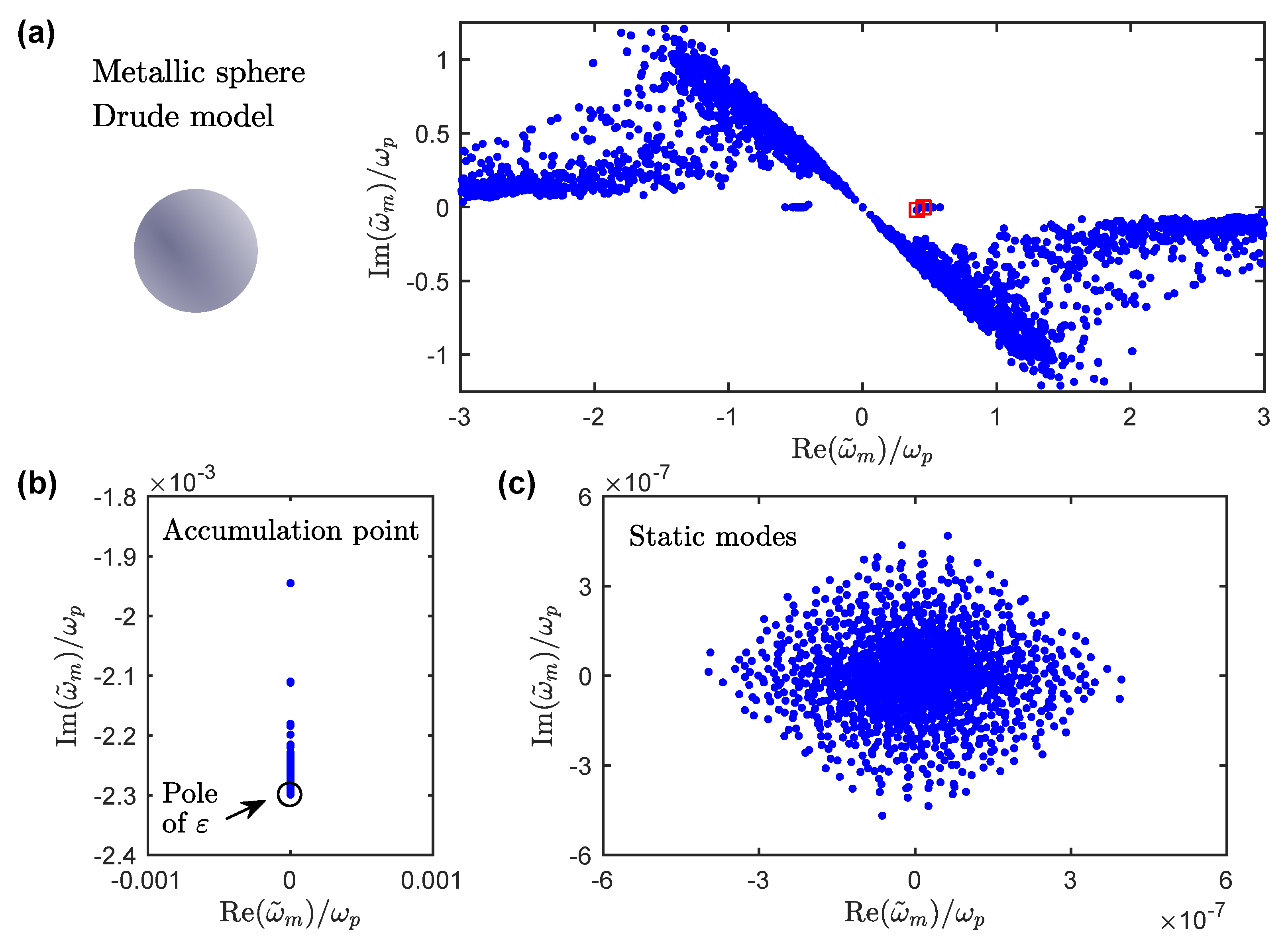
Figure 1a displays all 6482 eigenfrequencies in the complex frequency plane. The shape of the eigenvalues spectrum is typical of a FEM-based QNM solver implemented with non-dispersive PMLs; see for instance results in [15] for comparison. The modes whose excitation is responsible for the two resonances observed in Figure 2a are highlighted with red squares. Most of the modes are “numerical” or “PMLs” modes; they have no clear physical meaning but are important to ensure the convergence of the QNM expansion.

Figure 1b,c show enlarged views of two specific area of the complex frequency plane. Eigenfrequencies forming an accumulation point at the pole $\omega =-i\gamma$ of the Drude permittivity are shown in Figure 1b. Eigenfrequencies with very small values close to the origin $\omega =0$ are shown in Figure 1c. The latter are the numerical versions of pure static modes calculated with the QNM solver: their eigenfrequencies are not strictly equal to zero due to numerical inaccuracies in the resolution of the eigenvalue problem.

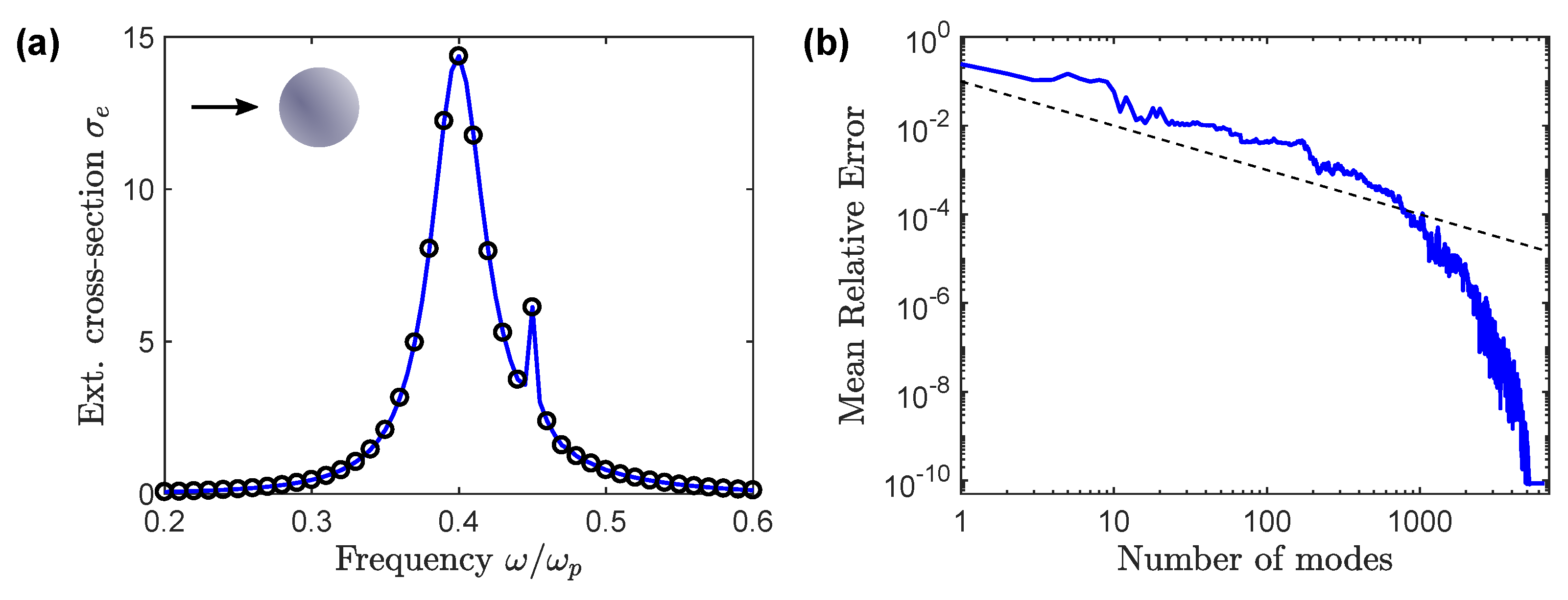
With these QNMs, we reconstruct the field scattered by the sphere illuminated with a linearly polarized plane wave; see Equations (7) and (8). Then, we calculate the extinction cross-section,

$${\sigma }_e=\frac{\omega }{2P_i}{\int \int \int }_{V_{\mathrm{res}}}\mathrm{Im}\left[\Delta \epsilon \mathbf{E}·{\mathbf{E}}_i^{*}\right]d^3\mathbf{r},$$

(9)

where $P_i=\frac{1}{2}{\epsilon }_{0}c{\left|{\mathbf{E}}_i\right|}^2$ is the Poynting vector norm of the incident plane wave in air and $\mathbf{E}$ is the total electric field inside the sphere. The extinction cross-section calculated with the QNM expansion is shown by the solid blue curve in Figure 2a. It exhibits two resonances that are caused by the excitation of the two QNMs highlighted by the red squares in Figure 1a. Black circles display the result of a direct FEM calculation of the cross-section with the same mesh. The agreement is excellent.

Finally, we investigate the convergence of the QNM expansion in Figure 2b. We plot the mean relative error as a function of the number of modes retained in the expansion. The results of the direct FEM calculation ${\sigma }_e^{\mathrm{FEM}}$ are used as a reference. Modes are sorted in descending order according to their contribution to the cross-section, which is given by $|{\int \int \int }_{V_{\mathrm{res}}}\mathrm{Im}\left[\Delta \epsilon {\alpha }_m{\tilde{\mathbf{E}}}_m·{\mathbf{E}}_i^{*}\right]d^3\mathbf{r}|$. The mean of the relative error over the spectral range considered in Figure 2a is calculated as $\frac{1}{M}{\sum }_{i=1}^M{\mathrm{Err}}_i$, with ${\mathrm{Err}}_i=|{\sigma }_e^{\mathrm{QNM}}\left({\omega }_i\right)-{\sigma }_e^{\mathrm{FEM}}\left({\omega }_i\right)|/{\sigma }_e^{\mathrm{FEM}}\left({\omega }_i\right)$ and $M=41$ the number of frequency points ${\omega }_i$ used in Figure 2a. To get an idea of the convergence speed, the black dashed line shows a $1/N$ decrease.

Two important conclusions can be drawn. First, the QNM expansion nicely converges towards the result of a direct FEM calculation with the same mesh. The mean relative error over a broad spectral range is as small as ${10}^{-10}$, which means that the scattered field is well reconstructed both on resonance and out of resonance. Secondly, static modes do not contribute to the field reconstruction and can be removed from the QNM expansion. Indeed, the modes whose eigenfrequency is close to zero (modes shown in Figure 1c) make a zero contribution to the cross-section. They are the last in the sorted list of QNMs; their addition to the modal expansion does not change the error, as can be seen from the bottom right corner of Figure 2b.

The uselessness of static modes can be explained as follows: $\omega =0$ is a pole of the Drude permittivity, and $\epsilon \left(0\right)\to \infty$. As a result, the electric field of static modes vanishes inside the metal, their excitation coefficient is equal to zero according to Equation (8), and they do not contribute to the QNM expansion. Since $\omega =0$ is not a pole of the Lorentz permittivity, we see in the next section that the situation is drastically different for a resonator made of a dielectric material.

3.2. Lorentz Permittivity—Dielectric Sphere

We consider now the dielectric nanosphere studied in [26]. The sphere of radius $R=75$ nm is embedded in air, and its frequency-dependent permittivity is given by a Lorentz model, $\epsilon \left(\omega \right)={\epsilon }_0{\epsilon }_{\infty }\left(1-\frac{{\omega }_p^2}{{\omega }^2-{\omega }_0^2+i\omega \gamma }\right)$, with ${\epsilon }_{\infty }=8.51$, ${\omega }_p=3.62\times {10}^{15}$ rad·s${}^{-1}$, ${\omega }_0=5.09\times {10}^{15}$ rad·s${}^{-1}$, and $\gamma =1.16\times {10}^{14}$ rad·s${}^{-1}$. The parameters of the Lorentz model have been chosen to fit the data of silicon tabulated in [32] in the 400–800 nm spectral range.

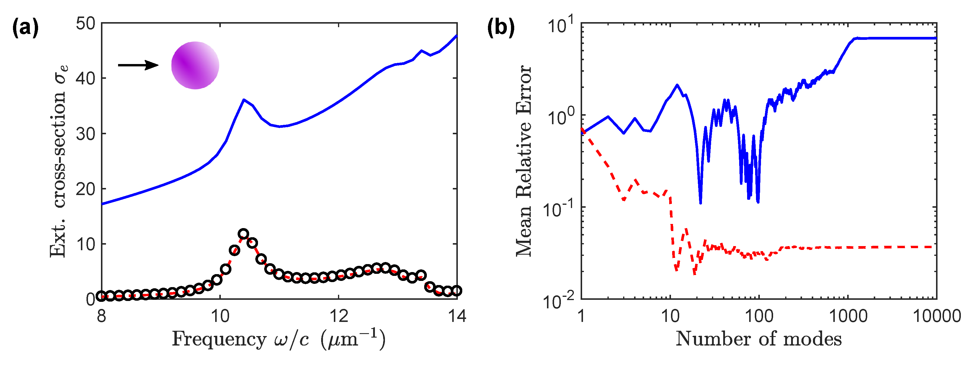
Figure 3a displays all 15,394 complex eigenfrequencies computed with the QNM solver. The shape of the eigenvalues spectrum is similar to that of the metallic sphere; most of the calculated modes are “PMLs” modes. Three QNMs are responsible for the resonances observed in Figure 4a; they are highlighted with red squares. Figure 3b,c show enlarged views of two specific areas of the complex frequency plane. Eigenfrequencies forming an accumulation point at the pole $\omega =\sqrt{{\omega }_0^2-{\gamma }^2/4}-i\gamma /2$ of the Lorentz permittivity are shown in Figure 3b. Eigenfrequencies with very small values close to the origin $\omega =0$ are shown in Figure 3c. The latter are the numerical versions of pure static modes calculated with the QNM solver; their eigenfrequencies are not strictly equal to zero due to numerical inaccuracies in the resolution of the eigenvalue problem.

With these modes, we reconstruct the field scattered by the sphere illuminated with a linearly polarized plane wave; see Equations (7) and (8). Then, we calculate the extinction cross-section with Equation (9). The extinction cross-section calculated with the complete QNM expansion is shown by the solid blue curve in Figure 4a. In that case, the QNM expansion provides an erroneous cross-section that is completely different from the results of a direct FEM calculation with the same mesh (black circles). The corresponding mean relative error (calculated as in the previous Section) is shown by the blue solid curve in Figure 4b. It is extremely large.

This dramatic disagreement is due to the incorrect calculation of the static modes’ contribution. Indeed, by comparing the field distributions with an exact analytical calculation [26], we have found that the static modes are incorrectly calculated by the QNM solver. As a result, their excitation coefficients and their contribution to the scattered field are erroneous. Removing these modes (the 1786 modes shown in Figure 3c) from the QNM expansion leads to a better reconstruction, as shown by the red dashed curve in Figure 4a. However, in the absence of static modes, the reconstruction cannot be accurate, as shown previously in [26]. The red dashed curve in Figure 4b illustrates that, with a QNM expansion that excludes static modes, the mean relative error does not decrease with the number of modes but on the contrary saturates to a value of a few percent.

Two important conclusions can be drawn. First, these results provide evidence that static modes make a non-negligible contribution to the scattered-field reconstruction in the case of a Lorentz permittivity. When a numerical QNM solver is used, their specific contribution is not replaced by other “numerical” modes. Secondly, static modes are incorrectly calculated by a numerical QNM solver designed to calculate modes with a non-zero eigenfrequency. It is of major importance to solve this issue if one wants to use QNM expansions for dielectric resonators. In the next section, we propose to add to the QNM solver a specific calculation of the static modes.

4. Specific Calculation of the Static Modes

In the case of dielectric systems, a QNM expansion without static modes is not accurate, as shown by the red dashed curve in Figure 4b and by the results in [26]. However, the static modes calculated by the QNM solver are erroneous and cannot be used.

We propose to use a separate, specific computation of the static modes to improve the accuracy of the QNM expansion in the case of dielectric systems. The calculation is performed by solving an electrostatic problem with the FEM; it is described in Section 4.1. This approach is validated by considering the dielectric nanosphere (Section 4.2) as well as a more complex geometry that is not analytically solvable: a dielectric nanodisk (Section 4.3).

4.1. Calculation of the Static Eigenproblem

Instead of relying on the most general Maxwell equations to calculate all modes, we calculate the static modes by considering an electrostatic problem. We solve the Laplace equation,

$$\mathbf{\nabla }·\left[\epsilon \left(0\right)\mathbf{\nabla }{\tilde{V}}_m\right]=0,$$

(10)

where ${\tilde{V}}_m$ is the electrostatic potential and $\epsilon \left(0\right)$ is the value of the permittivity at $\omega =0$. In the case of a Lorentz permittivity, $\epsilon \left(0\right)={\epsilon }_0{\epsilon }_{\infty }(1+{\omega }_p^2/{\omega }_0^2)$. By using the FEM formulation, Equation (10) is recast into a matrix eigenvalue problem for which we calculate the zero eigenvalues.

For a resonator embedded in a homogeneous medium, the electrostatic potential outside the structure varies asymptotically as ${\tilde{V}}_m\sim a/r$ and cancels out at infinity. Therefore, it is not necessary to use PMLs, and we solve Equation (10) with the following boundary condition in the FEM formulation:

$$\frac{\partial {\tilde{V}}_m}{\partial r}=-\frac{{\tilde{V}}_m}{r}.$$

(11)

Once the distribution of the potential is known, we calculate the electric field of the static modes as

$${\tilde{\mathbf{E}}}_m^{st}=-\mathbf{\nabla }{\tilde{V}}_m.$$

(12)

Since static modes do not diverge as $r\to \infty$, they can be normalized easily without regularization. They are normalized with Equation (3) by using the fact that ${\tilde{\mathbf{H}}}_m^{st}=0$. Finally, their excitation coefficient is calculated with Equation (8).

We validate this specific calculation of static modes in the following two sections.

4.2. Back to the Dielectric Sphere

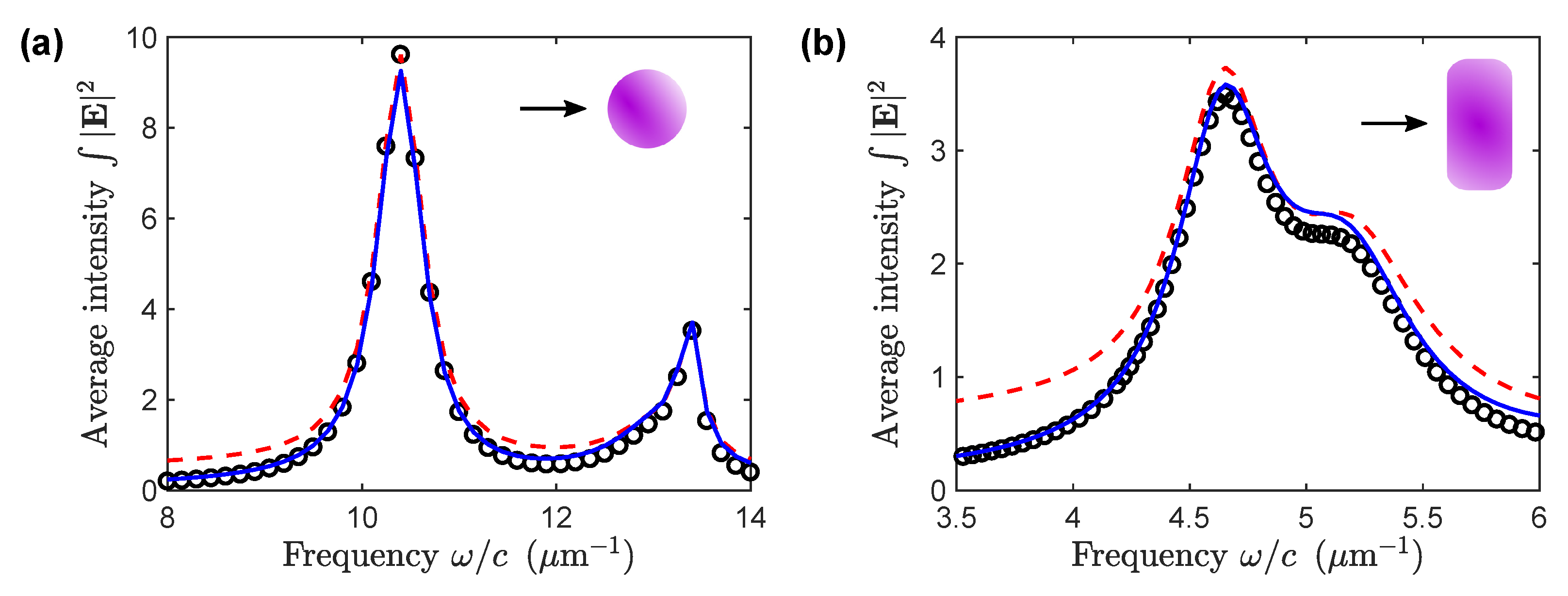
Let us come back to the case of the dielectric sphere of Section 3.2. We reconstruct the scattered field with a QNM expansion formed by all non-static modes of Figure 3 (all modes excluding the 1786 static modes shown in Figure 3c), to which we add 90 static modes computed with the method described in Section 4.1. To validate this approach, we have chosen to calculate the average intensity enhancement inside the resonator, $(1/V_{\mathrm{res}}){\int }_{V_{\mathrm{res}}}{\left|\mathbf{E}\right|}^2/{\left|{\mathbf{E}}_i\right|}^2{d}^3\mathbf{r}$, because static modes significantly contribute to this physical quantity [26]. The sphere is illuminated by a linearly polarized plane wave.

Figure 5a displays the average intensity enhancement inside the sphere as a function of the frequency. The results of a direct FEM calculation (black circles) are taken as a reference. The red dashed curve shows the inaccurate results obtained with a QNM expansion that excludes static modes, and the blue curve shows the results obtained by combining non-static modes calculated with the QNM solver and 90 static modes computed separately. The proposed method to calculate static modes works well and allows for an improvement of the field reconstruction inside the sphere.

4.3. A More Complex Geometry—Dielectric Disk

To further validate our approach, we study a more complex geometry that is not analytically solvable. We consider a silicon nanodisk that has been previously studied in [33], with a radius of 242 nm, a height of 220 nm, and rounded edges with a radius of 50 nm. The silicon permittivity is described by the Lorentz model used in Section 3.2. As for the sphere, we calculate the average intensity enhancement inside the object as a function of the frequency. The incident plane wave has its wave vector parallel to the axis of the disk and it is linearly polarized.

The results are displayed in Figure 5b. The red dashed curve shows the inaccurate results obtained with a QNM expansion that excludes static modes and the blue curve shows the results obtained by combining non-static modes calculated with the QNM solver and static modes computed separately. A direct FEM calculation (black circles) is taken as a reference. Again, adding in the QNM expansion static modes that are computed separately improves the accuracy of the field reconstruction.

5. Conclusions

We have studied the calculation and the role of static modes in the electromagnetic field reconstruction in the case where a numerical QNM solver is used. We have shown that static modes do not contribute to the field reconstruction in the case of a resonator made of a metallic material whose permittivity is described by a Drude model. The calculation of static modes is thus useless in that case. We have shown that the situation is drastically different in the case of a resonator made of a dielectric material whose permittivity is described by a Lorentz model. Static modes markedly contribute to the field reconstruction but are incorrectly calculated with a QNM solver designed to compute modes with non-zero eigenfrequencies. To our knowledge, this important issue had not been been raised until now.

Therefore, for dielectric resonators, QNM expansions should be used by paying special attention to static modes. To bypass this issue, we have proposed the use of a separate, specific computation of the static modes. We have validated our approach numerically on two different examples: a dielectric nanosphere and a dielectric nanodisk. We have focused our work on purely metallic and purely dielectric resonators. An interesting perspective would be to study metallo-dielectric structures.

References

- Khajavikhan, M.; Simic, A.; Katz, M.; Lee, J.H.; Slutsky, B.; Mizrahi, A.; Lomakin, V.; Fainman, Y. Thresholdless nanoscale coaxial lasers. Nature 2012, 482, 204–207. [Google Scholar] [CrossRef] [PubMed]
- Hill, M.T.; Gather, M.C. Advances in small lasers. Nat. Photonics 2014, 8, 908–918. [Google Scholar] [CrossRef]
- Liu, N.; Tang, M.L.; Hentschel, M.; Giessen, H.; Alivisatos, A.P. Nanoantenna-enhanced gas sensing in a single tailored nanofocus. Nat. Mater. 2011, 10, 631–636. [Google Scholar] [CrossRef] [PubMed]
- Alessandri, I.; Lombardi, J.R. Enhanced Raman Scattering with Dielectrics. Chem. Rev. 2016, 116, 14921–14981. [Google Scholar] [CrossRef]
- Neubrech, F.; Huck, C.; Weber, K.; Pucci, A.; Giessen, H. Surface-Enhanced Infrared Spectroscopy Using Resonant Nanoantennas. Chem. Rev. 2017, 117, 5110–5145. [Google Scholar] [CrossRef]
- Leung, P.T.; Liu, S.Y.; Young, K. Completeness and orthogonality of quasinormal modes in leaky optical cavities. Phys. Rev. A 1994, 49, 3057–3067. [Google Scholar] [CrossRef]
- Lalanne, P.; Yan, W.; Vynck, K.; Sauvan, C.; Hugonin, J.P. Light Interaction with Photonic and Plasmonic Resonances. Laser Photonics Rev. 2018, 12, 1700113. [Google Scholar] [CrossRef]
- Sauvan, C.; Wu, T.; Zarouf, R.; Muljarov, E.A.; Lalanne, P. Normalization, orthogonality, and completeness of quasinormal modes of open systems: The case of electromagnetism. Opt. Express 2022, 30, 6846–6885. [Google Scholar] [CrossRef]
- Muljarov, E.A.; Langbein, W.; Zimmermann, R. Brillouin-Wigner perturbation theory in open electromagnetic systems. Europhys. Lett. 2010, 92, 50010. [Google Scholar] [CrossRef]
- Sauvan, C.; Hugonin, J.P.; Maksymov, I.S.; Lalanne, P. Theory of the Spontaneous Optical Emission of Nanosize Photonic and Plasmon Resonators. Phys. Rev. Lett. 2013, 110, 237401. [Google Scholar] [CrossRef] [Green Version]
- Bai, Q.; Perrin, M.; Sauvan, C.; Hugonin, J.P.; Lalanne, P. Efficient and intuitive method for the analysis of light scattering by a resonant nanostructure. Opt. Express 2013, 21, 27371–27382. [Google Scholar] [CrossRef]
- Doost, M.B.; Langbein, W.; Muljarov, E.A. Resonant-state expansion applied to three-dimensional open optical systems. Phys. Rev. A 2014, 90, 013834. [Google Scholar] [CrossRef]
- Muljarov, E.A.; Langbein, W. Exact mode volume and Purcell factor of open optical systems. Phys. Rev. B 2016, 94, 235438. [Google Scholar] [CrossRef]
- Mansuripur, M.; Kolesik, M.; Jakobsen, P. Leaky modes of solid dielectric spheres. Phys. Rev. A 2017, 96, 013846. [Google Scholar] [CrossRef]
- Yan, W.; Faggiani, R.; Lalanne, P. Rigorous modal analysis of plasmonic nanoresonators. Phys. Rev. B 2018, 97, 205422. [Google Scholar] [CrossRef]
- Zolla, F.; Nicolet, A.; Demésy, G. Photonics in highly dispersive media: The exact modal expansion. Opt. Lett. 2018, 43, 5813–5816. [Google Scholar] [CrossRef]
- Abdelrahman, M.I.; Gralak, B. Completeness and divergence-free behavior of the quasi-normal modes using causality principle. OSA Contin. 2018, 1, 340–348. [Google Scholar] [CrossRef]
- Lobanov, S.V.; Langbein, W.; Muljarov, E.A. Resonant-state expansion of three-dimensional open optical systems: Light scattering. Phys. Rev. A 2018, 98, 033820. [Google Scholar] [CrossRef]
- Zschiedrich, L.; Binkowski, F.; Nikolay, N.; Benson, O.; Kewes, G.; Burger, S. Riesz-projection-based theory of light-matter interaction in dispersive nanoresonators. Phys. Rev. A 2018, 98, 043806. [Google Scholar] [CrossRef]
- Weiss, T.; Muljarov, E.A. How to calculate the pole expansion of the optical scattering matrix from the resonant states. Phys. Rev. B 2018, 98, 085433. [Google Scholar] [CrossRef] [Green Version]
- Colom, R.; McPhedran, R.; Stout, B.; Bonod, N. Modal expansion of the scattered field: Causality, nondivergence, and nonresonant contribution. Phys. Rev. B 2018, 98, 085418. [Google Scholar] [CrossRef]
- Zimmerling, J.; Remis, R. Modal analysis of photonic and plasmonic resonators. Opt. Express 2020, 28, 20728–20737. [Google Scholar] [CrossRef] [PubMed]
- Truong, M.D.; Nicolet, A.; Demésy, G.; Zolla, F. Continuous family of exact Dispersive Quasi-Normal Modal (DQNM) expansions for dispersive photonic structures. Opt. Express 2020, 28, 29016–29032. [Google Scholar] [CrossRef] [PubMed]
- Gras, A.; Lalanne, P.; Duruflé, M. Nonuniqueness of the quasinormal mode expansion of electromagnetic Lorentz dispersive materials. J. Opt. Soc. Am. A 2020, 37, 1219–1228. [Google Scholar] [CrossRef]
- Defrance, J.; Weiss, T. On the pole expansion of electromagnetic fields. Opt. Express 2020, 28, 32363–32376. [Google Scholar] [CrossRef]
- Sauvan, C. Quasinormal modes expansions for nanoresonators made of absorbing dielectric materials: Study of the role of static modes. Opt. Express 2021, 29, 8268–8282. [Google Scholar] [CrossRef]
- Wu, T.; Arrivault, D.; Duruflé, M.; Gras, A.; Binkowski, F.; Burger, S.; Yan, W.; Lalanne, P. Efficient hybrid method for the modal analysis of optical microcavities and nanoresonators. J. Opt. Soc. Am. A 2021, 38, 1224–1231. [Google Scholar] [CrossRef]
- Lobanov, S.V.; Langbein, W.; Muljarov, E.A. Resonant-state expansion applied to three-dimensional open optical systems: Complete set of static modes. Phys. Rev. A 2019, 100, 063811. [Google Scholar] [CrossRef]
- Yan, W.; Lalanne, P.; Qiu, M. Shape deformation of nanoresonator: A quasinormal-mode perturbation theory. Phys. Rev. Lett. 2020, 125, 013901. [Google Scholar] [CrossRef]
- Lalanne, P.; Yan, W.; Gras, A.; Sauvan, C.; Hugonin, J.P.; Besbes, M.; Demésy, G.; Truong, M.D.; Gralak, B.; Zolla, F.; et al. Quasinormal mode solvers for resonators with dispersive materials. J. Opt. Soc. Am. A 2019, 36, 686–704. [Google Scholar] [CrossRef]
- Demésy, G.; Nicolet, A.; Gralak, B.; Geuzaine, C.; Campos, C.; Roman, J.E. Non-linear eigenvalue problems with GetDP and SLEPc: Eigenmode computations of frequency-dispersive photonic open structures. Comput. Phys. Commun. 2020, 257, 107509. [Google Scholar] [CrossRef]
- Green, M.A.; Keevers, M.J. Optical Properties of Intrinsic Silicon at 300 K. Prog. Photovolt. Res. Appl. 1995, 3, 189–192. [Google Scholar] [CrossRef]
- Powell, D.A. Interference between the Modes of an All-Dielectric Meta-atom. Phys. Rev. Appl. 2017, 7, 034006. [Google Scholar] [CrossRef] [Green Version]
Figure 1.
Complex QNM frequencies for a metallic sphere with a Drude permittivity. (a) Full eigenvalues spectrum computed with the QNM solver. Red squares show the two QNMs responsible for the resonances observed in the spectral range of interest. (b) Eigenvalues forming an accumulation point at the pole of the permittivity. (c) Cloud of eigenvalues close to the origin that correspond to static modes.
Figure 2.
Convergence of the QNM expansion for a metallic sphere with a Drude permittivity. (a) Spectrum of the extinction cross-section normalized by the sphere apparent surface . The results obtained with the QNM expansion (blue curve) are compared with the results of a direct FEM calculation (black circles). (b) Mean relative error as a function of the number of modes retained in the QNM expansion. The results of a direct FEM calculation with the same mesh are taken as a reference, and the relative error is averaged over the spectral range of (a). The black dashed line shows a decrease.
Figure 3.
Complex QNM frequencies for a dielectric sphere with a Lorentz permittivity. (a) Full eigenvalues spectrum computed with the QNM solver. Red squares show the three QNMs responsible for the resonances in the spectral range of interest. (b) Eigenvalues forming an accumulation point at the pole of the permittivity. (c) Cloud of eigenvalues close to the origin that correspond to static modes.
Figure 4.
Convergence of the QNM expansion for a dielectric sphere with a Lorentz permittivity. (a) Spectrum of the extinction cross-section normalized by the sphere apparent surface . The results obtained with the QNM expansion formed with all modes shown in Figure 3a (blue curve) are compared with the results of a direct FEM calculation (black circles). The red dashed curve displays the results obtained with a QNM expansion that excludes the 1786 static modes shown in Figure 3c. (b) Mean relative error as a function of the number of modes retained in the QNM expansion. With the static modes calculated with the QNM solver (blue curve) and without them (red dashed curve). The results of a direct FEM calculation with the same mesh are taken as a reference and the relative error is averaged over the spectral range of (a).
Figure 5.
Field reconstruction with a specific computation of the static modes. (a) Dielectric nanosphere of Section 3.2. (b) Dielectric nanodisk with rounded edges. The average intensity enhancement inside the resonator is plotted as a function of the frequency, . Blue curve: QNM expansion with separately computed static modes; Red dashed curve: QNM expansion without static modes; Black circles: direct FEM calculation.
Publisher’s Note: MDPI stays neutral with regard to jurisdictional claims in published maps and institutional affiliations. |
© 2022 by the authors. Licensee MDPI, Basel, Switzerland. This article is an open access article distributed under the terms and conditions of the Creative Commons Attribution (CC BY) license (https://creativecommons.org/licenses/by/4.0/).
Share and Cite
MDPI and ACS Style
Besbes, M.; Sauvan, C. Role of Static Modes in Quasinormal Modes Expansions: When and How to Take Them into Account? Mathematics 2022, 10, 3542. https://doi.org/10.3390/math10193542
AMA Style
Besbes M, Sauvan C. Role of Static Modes in Quasinormal Modes Expansions: When and How to Take Them into Account? Mathematics. 2022; 10(19):3542. https://doi.org/10.3390/math10193542
Chicago/Turabian StyleBesbes, Mondher, and Christophe Sauvan. 2022. "Role of Static Modes in Quasinormal Modes Expansions: When and How to Take Them into Account?" Mathematics 10, no. 19: 3542. https://doi.org/10.3390/math10193542
Note that from the first issue of 2016, this journal uses article numbers instead of page numbers. See further details here.