
A Quantum Planner for Robot Motion
by
 , , , and
Antonio Chella
1,2 ,
,
Salvatore Gaglio
1,2,
Giovanni Pilato
2,
Filippo Vella
2,* and
Salvatore Zammuto
1 1
Dipartimento di Ingegneria (DID), Università degli Studi di Palermo, 90128 Palermo, Italy
2
Istituto di Calcolo e Reti ad Alte Prestazioni (ICAR), Consiglio Nazionale delle Ricerche (CNR), Via Ugo La Malfa 153, 90146 Palermo, Italy
*
Author to whom correspondence should be addressed.
Mathematics 2022, 10(14), 2475; https://doi.org/10.3390/math10142475
Submission received: 1 April 2022
/
Revised: 8 July 2022
/
Accepted: 9 July 2022
/
Published: 16 July 2022
(This article belongs to the Special Issue Advances in Quantum Artificial Intelligence and Machine Learning)
Abstract
:The possibility of integrating quantum computation in a traditional system appears to be a viable route to drastically improve the performance of systems endowed with artificial intelligence. An example of such processing consists of implementing a teleo-reactive system employing quantum computing. In this work, we considered the navigation of a robot in an environment where its decisions are drawn from a quantum algorithm. In particular, the behavior of a robot is formalized through a production system. It is used to describe the world, the actions it can perform, and the conditions of the robot’s behavior. According to the production rules, the planning of the robot activities is processed in a recognize–act cycle with a quantum rule processing algorithm. Such a system aims to achieve a significant computational speed-up.
1. Introduction
The planning of the actions that a robot can accomplish to reach a defined goal is a traditional problem that has been tackled since the first robots were built [1]. In the case of motion planning, the robot moves in a known environment and it has to perform suitable actions to reach a goal destination [2,3]. The actions that the robot can perform are bound to the degrees of freedom of the robot. In the formulation we consider, the movements are executed on a plane where impenetrable and immovable obstacles are present. If b is the number of possible actions that the robot can choose and d is the number of steps, the complexity is bound to . Here, we consider a mobile robot placed on a map that through suitable movements, chosen by a quantum algorithm, has to reach a target position. This path planning problem can be equivalently formulated either as the computation of the trajectory the robot will take or as the sequence of actions (i.e., the moves) the robot should carry out to reach the goal. We chose to operate in accordance with the latter of the two formulations since it best assimilates the philosophy of a production system [4]. A production system is a computational formalism that is extremely popular in AI due to its inherent capability of modeling a human-like flow of thought when it comes to the activity of problem solving [5] and is equivalent to the Universal Turing Machine (UTM) [6].
A production model essentially relies upon the cyclic application of production rules, i.e., condition-action pairs where a system is transformed into a specific state when the current state has validated one (or more) condition(s) and, according to the predefined productions, suitable action are applied. This process is done iteratively until either no further condition is met or when a specific target state has been reached. Such a procedure is also referred to as the recognize–act cycle (RAC).
As reported by [7], the task of identifying the best actions to achieve a given goal requires significant use of computing capabilities. This statement is even more relevant when agents act in complex environments. With this in mind, Manin [8] proposed to employ quantum computing processes. In [7], a possible problem-solving technique is introduced, approached from the point of view of quantum computation. The proposed approach also starts from considerations raised in Ying [9], regarding the link between artificial intelligence and quantum computation and is based on the theory of production systems. This formalism, proposed by Post [4], introduces computational procedures and exploits problem-solving primitives. Production systems are widely used in the context of classical artificial intelligence and cognitive psychology. In particular, they describe how to construct a sequence of actions that, from an initial state, leads to a goal state. This formalism is also one of the most successful computer models for representing human behavior in problem-solving cases [10]. A classical production system consists of rules, also called “productions”. One of the most common planning methodologies is the Stanford Research Institute Problem Solver (STRIPS) technique, introduced in [11]. This kind of production system can be represented with a search tree, that is rooted at the current system state and has a branching factor given by the actions that can be applied at each state [12]. It is clear that, as the depth of the tree increases, the number of reached states grows exponentially. Many traditional algorithms afford the search in these trees and they range from brute force search to most refined techniques. Quantum search in trees is described in [13,14]. A model capable of solving instances of the n-puzzle, was proposed in [7]. The initial state is the root node, the branches of each node represent the possible rules that can be applied in a particular state, while the goal(s) are encoded in a subset of the leaf nodes. Such a model combines a quantum search mechanism with production system theory. In particular, it exploits the quantum superposition principle, exploring all possible combinations of initial configurations and paths according to the desired depth level. A quantum backtracking search, that can be seen as a depth-first search in a tree with a pruning of dead-end nodes, is proposed in [15]. A random walk to solve backtracking algorithms has been proposed in [16,17].
In this paper, we illustrate a methodology which integrates quantum computation in a traditional robotic system. We explore a robot navigation task in an environment, such as the one shown in Figure 1, where the robot takes its decisions by using a quantum approach. In particular, the technique is based on Grover’s algorithm [18] and it is used to plan the movements of the robot on the map where it lives. The behavior of a robot is formalized through a production system, which is used to describe the world, the actions it can perform, and the conditions of its behavior. According to the production rules, the planning of the robot activities is processed in a recognize-act cycle with a quantum rule processing algorithm. Such an approach can significantly improve the computational performance of systems endowed with artificial intelligence. The employment of quantum algorithms in this framework is motivated by the strong affinity between quantum theory and the inner mechanics of (human) reasoning, due mainly to its characteristic parallel processing. From the implementation point of view, the idea is to study the feasibility of the methodology, realizing a proof-of-concept prototype in an emulated environment or exploiting a set of proper calls to the IBM Qiskit service [19].
The contributions of this work are: (1) a formulation of the path-planning problem that solves through a quantum algorithm; (2) the application of Grover’s theoretical procedure to a practical problem, together with some strategies to tackle them; (3) the evaluation of the conditions for effectiveness of the quantum search algorithm for the search in a tree used to model the robotic path planning. In addition, in Section 2.1 we present a general approach for encoding traditional Boolean combinatorial networks into equivalent quantum circuits exploiting the quantum parallelism property of superposed quantum states. We also examine the constraints of quantum circuit design, such as the optimal choice of circuit gates and the reversibility constraint of quantum computation. After the descriptions of the quantum path planning procedure, in Section 7 we provide an extensive discussion on the efficacy and success probability of the approach, along with its effectiveness for the state-of-the-art quantum hardware and simulation technologies. A novel technique that enables the classical simulation of complex quantum circuits, reusing qubits and reducing the needed memory resources is also described.
2. Materials and Methods
In the following subsections, we illustrate the basic concepts about quantum gates and how they can be used to implement traditional Boolean logic, together with the role of quantum computation in tree-search procedures and an overview of the role of Grover’s algorithm in search problems.
2.1. Quantum Computation and Boolean Networks
The possibility to adopt quantum computation for traditional tasks enables to rethink computing models and speed up cumbersome computations [12,13,20,21,22,23]. The characteristics of quantum computing allow us to solve traditional problems with models that manage multiple configurations of the variables at the same time and select, in a single step, the problem solution, implementing the usually called quantum parallelism [21,24]. This capability is based on the property of physical quantities, as the elements of quantum mechanics, to combine or superpose two or more quantum states, creating a new valid quantum state in accordance with the Schrödinger equation.
A single unit of information , or qubit, is represented by a vector in a 2D Hilbert space and thus requires a total of two complex numbers to encode its coordinates with respect to one of the space’s bases, usually the so-called computational (or Z-) basis, related to the observable states of the form . A state, that is a linear combination of the Z-basis, such as , can be arbitrarily transformed into another state until a measurement is performed, which collapses the wavefunction to one of the observables, each with probability amplitudes and .
These amplitudes satisfy the unitarity constraint of probability [25]. The two complex numbers and , whose combination is a fixed-magnitude vector in a 3D Euclidean space, trace out a geometric locus that corresponds to a unitary sphere, namely, the Bloch sphere [26] (Figure 2).
A single-qubit gate is thus a unitary (and subsequently reversible) operator (see Section 2.2 for a discussion on quantum gates reversibility) that performs some rotation of the input state over the Bloch sphere around one or more of the X, Y, and Z axes. An example is given by the Pauli-X gate, which is associated to a rotation of radians around the X axis of the sphere, a behavior, that when applied to a computational-basis state, is equivalent to the classical operation. Another quantum gate of interest is the Hadamard gate H, which performs a rotation around the Y axis, followed by a rotation around the X axis. For this reason, the H gate often serves the purpose of preparing an (observable) input state as a uniform superposition, one where , since it operates by bringing a point from the Z-axis to the plane, exactly halfway between the and states of the sphere. Applying an Hadamard operation on results in a state that is a combination of the individual outputs of the gate as if they had been transformed one at a time, which realizes the aforementioned property of quantum parallelism of quantum circuits. This effect is more noticeable for n-qubit gates, where a single application of an operator acts simultaneously on all of the components of the input state. At the time of measurement, only one of such states is selected, according to its relative probability amplitude. For this reason, the quantum circuits that implement quantum algorithms are designed in the interest of exploiting the constructive or destructive interference phenomena that occur when multiple wavefunctions are combined, so that the probability of measuring a desired solution is increased, while everything else is being diminished.
This methodology allows the quantum programmer to process, in a single step, an exponential number of input configurations—where the exponent is given by the number of the input qubits—and select among them the values that produce the desired output. At the same time, conceiving an algorithm that harnesses this quantum parallelism needs some specific settings to shape the computation strictly in terms of the constraints of quantum technology, such as unitarity and thus reversibility of quantum operators. Here, the qubit information is processed through quantum gates that have been composed to implement a logical computation over its corresponding quantum circuit. As such, not all the traditional logic gates are directly available and some of them, such as the logical , must be mapped to the existing quantum gates. One way of implementing a traditional method with a quantum computer is to construct a classical Boolean network and then substitute its logic with quantum gates. This is completed by either directly replacing the gates, when available, or by performing Boole algebra manipulations on the starting logic with the objective of obtaining an expression that contains just the operators that can be mapped to the accessible quantum gates.
With this in mind, in this work we choose to exploit the elementary quantum gates (respectively, the X gate, the Toffoli gate and the gate), together with the functional completeness of the set of connectives to realize our Boolean logic as a quantum combinatorial circuit through the association:
In particular:
- the directly translates to the X gate, which flips the phase of its input around the X axis of the Bloch sphere;
- the Toffoli () acts on the target qubit when both of its control bits are set to 1. This is the same behavior of a reversible operation;
- the classical operation can be implemented reversibly with a 3-qubit gate, where two s, one for each input, control the same output bit (rightmost subfigure of Figure 3).
Expression (1) sums up the aforementioned strategy for the adaptation of traditional logic to a quantum network: we take advantage of the universality of the set by reducing the classical combinatorial logic in terms of these operations, and then replacing them with their quantum equivalents, , which are thereupon also universal [28]. In consideration of the fact that the C set is functionally complete, any other set that contains it must also be complete, this is why, for convenience reasons, we also incorporate the gate in our translation scheme, since it is a recurrent operation in our path-planning logic and it is useful to have a fixed reference to it and its quantum gate realization. Not unexpectedly, there exist many universal sets of quantum gates [21,29], some of which have elements that do not have a classical logical analogue and that can also be used to design a quantum algorithm that solves problems of the same kind. Nonetheless, they might not be as suitable in respect of design complexity concerns, in the sense that traditional logic offers a more solid frame of work to build highly-composite networks, along with well-explored optimization techniques that are particularly significant in the context of quantum algorithms, as discussed in Section 7. Additionally, out of the set we considered only , the Toffoli gate, that is a non-Clifford gate, since it is built on T gates ( rotation about the Z axis), which do not belong to the Clifford group [30]. The Gottesman–Knill theorem [31] states that gates outside of the Clifford group cannot be efficiently simulated by classical machines, therefore, a quantum circuit that minimizes the number of non-Cliffords gates can also benefit from better-performing classical simulations. In the implementations of Section 4 and Section 5, we show that indeed the great majority of heavy-duty computation is composed of the X and Clifford gates, with the Toffoli gate being involved mainly in aggregation and marking operations, which are much rarer if compared to the actual computation of the movements and position of the robot in the path-planning procedure.
2.2. Gate Reversibility
Reversibility is a core aspect of quantum mechanics [32,33] and studies on pure quantum states, as those related to the no-hiding theorem [34], observed that no information is lost during a state’s evolution in time; also, it is not possible for two different starting states to evolve to the same state through the same Hamiltonian.
Furthermore, quantum mechanics is unitary. Mathematically, unitarity means that any (simple or complex) U operation must satisfy , that also implies the condition of reversibility [21]. In any quantum algorithm, whether we consider the general operators or the exact Boolean functions they implement, reversibility, almost in all cases, requires the employment of additional ancillary qubits. This is because traditional gates often perform many-to-one bit mapping, with more general operations implementing a function for some fixed k, l number of input and output bits [7,35]. A configuration where prevents the bijection that allows to uniquely recover the input from the produced output. It follows that, in order to render a given irreversible operation reversible, supplementary bits within the gate are needed so that . One straightforward example is the classical operation, famously not reversible, and its quantum equivalent, the previously mentioned Toffoli gate, which takes a total of 3 bits as input (and output) against the 2 inputs and 1 output of the classical counterpart.
2.3. Quantum Path Planning
In the context of our problem, we designed a path-planning procedure starting from the traditional Boolean representation of the production rules that dictate the behavior of a robot’s movement. Then, we built the corresponding quantum network according to the translation scheme of Section 2.1, along with the adaptation to reversible computation of Section 2.2. In order to perform an exhaustive search across the entire map, the production rules that transform the state of the robot (that is, the position of the map cell it is located in) in a single RAC iteration, are of the type:
and
where a cell is considered “accessible” if it is within the walls of the map and does not have an obstacle in it. Rules of this kind are used to determine the behavior for each of the directions that movement is allowed towards.
In accordance with the forward-chaining nature of the repeated application of the RAC, it should be trivial to see that the overall control architecture of the system we just described results in a tree-like structure [12], with the initial state being the root node, the branches of each node representing the possible actions that can be carried out from that particular state, and the goal(s) being encoded in a subset of the leaf nodes. The computation halts in the case of target-state realization or, also, if no defined rule can be applied. In this sense, planning the optimal path from the robot’s starting position to the goal is equivalent to finding the shortest path from the root to a leaf node that corresponds to a target state, which can in turn be interpreted as a classical tree-search procedure, that our methodology solves through the application of the quantum search algorithm, namely, Grover’s algorithm.
2.4. Grover’s Algorithm
Grover’s algorithm [18] was conceived to solve the unstructured search problem through quantum processing [21]. Traditional unstructured search, or search on an unsorted database, requires a cost of in time, with N being the size of the search space. Quantum search provides a quadratic speed-up over its classical counterparts and it can be used to efficiently solve the NP-complete problems that require an exhaustive coverage of the search space. Considering a set of N entries, the algorithm works within an N-dimensional Hilbert space encoded by qubits. The states that correspond to the entries are represented as
Like many other quantum algorithms, quantum searching is based on constructing an operator that evolves the initial input state into a specific target state. Specifically, the Grover operator G takes as input , the initial superposition of the elements in the search space, and then evolves it into the solution state according to the Hamiltonian . If there is more than one solution, will be a combination of all the individual solution states [21]. The effect of such transformation is the rotation of the initial vector towards the solution .
This computation is implemented on a quantum computer by noticing that, since and belong to the same N-dimensional Hilbert space, we can easily perform a Gram–Schmidt orthonormalization to express in terms of the orthonormal basis , so that:
for some and with . Expression (3) can also be interpreted as follows: given that the initial is the superposition of all the states in the search space, must also be contained in such superposition. We can therefore express as the combination of the solution state , weighted with probability , together with a state that contains everything that is not a solution, , that has a probability of being measured.
On the hypothesis that the initial superposition of the N elements of the search space is uniform, and considering a generic number of solutions S of the problem, we can refactor expression (3) as
with and , where is the set of all of the solution states () and is its complement (). Since we assumed the uniformity of the starting superposition, if we were to perform measurement at time , the system’s state would collapse into any of the search states with equal probability . It is through the amplitude amplification technique that the quantum search algorithm is able to significantly enhance the probability of measuring a solution state, and, at the same time, due to unitarity of probability, to lower the expectation of non-solutions.
The system’s state can be visualized in terms of the 2D subspace generated by as a vector in the 2D plane spanned by and , which are orthonormal by construction, as seen in Figure 4.
Since S is typically much lower than N, the angle between and is small, which is the same as saying that initially, measuring a state that is not a solution is much more probable than measuring .
One way of looking at the rotation induced by the H Hamiltonian that we introduced at the start of this section, is by interpreting it as a double reflection, one with respect to and the other in the opposite direction, about the vector. As such, we define G as the Grover operator, i.e., the operator that rotates according to the two reflections and so that . Employing this operator a certain number of times will eventually rotate until it overlaps with , meaning that measurement at that time will output the solution state with near-certainty. It can be shown [21], on the assumption that , that such procedure is able to evolve to after a number R of rotations that has an upper bound equal to
Building a Grover operator, therefore, resolves to constructing the individual and operators, namely, the oracle and the diffuser.
In general terms, the oracle is an operator that marks the solution(s) of the search problem in accordance with the association [21]:
where is the register we want to search on, is the oracle qubit, ⊕ denotes addition modulo 2, and is a function such that is 1 if and 0 elsewhere; in other words, flips the phase of the oracle qubit if x is a solution. As for , while we normally initialize it to the state, such that we can detect a marked state by checking if has flipped it to the state, it is useful, in order to take advantage of the phase kickback effect within the context of the algorithmic procedure we are constructing, to set the initial state of as with [36]. When x is not a solution, applying the oracle to leaves the state unchanged, whereas if x is a solution for the search problem, and are interchanged, and the resulting state becomes , i.e.,
On account of the fact that the state itself is not affected by the controlled operation (rather, it influences through phase kickback), it can be omitted from the description, so that the expression that describes the actual action of the oracle on the input register now becomes:
This is equivalent to saying that the oracle marks a solution by inverting its phase once it recognizes it. The effect of applying to according to expression (8) geometrically corresponds to the reflection of about the vector. The other factor of the Grover operator is the diffuser , whose job is to execute the second reflection about , which is done with
This results from a basis change of the state to the computational or Z-basis through the Hadamard transform , subsequently applying a conditional phase shift, that is, a phase shift of -1 to every element of the Z-basis except for , defined as
that performs the mapping , where is the Kronecker delta on the states x and 0, and then re-applying to get back to . This is achieved on a quantum computer with the support of the gate, which inverts only the phase of the state , so that (10) is associated with
which means ignoring the global phase -1,
This is a convenient formulation, since the diffusion operator is standardized and not problem-specific, as opposed to the oracle , whose design is the main concern when applying Grover’s algorithm to a problem. The complete structure of a Grover operator G is represented in Figure 5. Grover’s quantum search can be carried out with oracle calls, as expressed in (5), and since it is proven that no search algorithm can achieve a complexity lower than , or it is , we know that the Grover procedure is optimal [21,37].
2.5. Harnessing the Quantum Advantage
The main reason behind the development of a quantum algorithm, apart from a pure conceptual interest, is that of the prospect of being able to solve fundamentally hard problems, such as path planning, both efficiently and in significantly reduced amounts of time. Although the computational power of quantum systems is theoretically proven to be superior with respect to any classically-achievable procedure [21,38], it is still unclear whether the actual construction of quantum machines powerful enough to achieve quantum supremacy is practically feasible (see Section 7.1 for a discussion on the issues of computation on quantum hardware). The authors of [39] simulated different instances of the hybrid QAOA [40] applied to the Max-Cut problem, artificially introducing “noise gates” to reproduce the effect of quantum decoherence of the physical quantum devices. They showed that no significant speed-up is attainable for noisy machines unless several hundreds of qubits are available. Although this is certainly not a promising outcome, it is worth bearing in mind that the evaluated results are only restricted to a specific procedure applied to solve a specific problem, and no inference can be made on the general computational capabilities of quantum computers whatsoever. More recently, Hlembotskyi et al. [41] investigated the performance of Grover’s algorithm on real quantum devices equipped with ion-trap technology, presenting encouraging data that demonstrate the actual improvements of the quantum search algorithm, which exceeds any possible classical approach even in the case of a single oracle call. Other studies have been made towards the exploration of the effectiveness of Grover’s algorithm, such as [42,43,44], and even a hardware efficient implementation has been proposed in [45], reducing the total depth and gate count of the circuit for the quantum search algorithm. All such experimental clues tilt the scales in favor of the actual, practical usefulness of Grover’s algorithm for real-world applications once more powerful and stabler quantum technologies are built [46,47], which, in the case of IBM’s quantum systems, should occur no longer than a handful of years, according to their 2025 quantum roadmap [48].
3. Planning Environment
The objective of the presented case study is the planning of the movement activities of a robotic entity that encode a path on a map through quantum computations. In that regard, a path is interpreted as the sequence of movements of the robot within a square grid map with obstacles, from the initial cell to the goal position (see Figure 1).
This environment is nicely described as a taxicab geometry [49], with the individual cells of the grid corresponding to the taxicab points and their adjacency being modeled by the connections between neighbor nodes. The main advantage of looking at the problem this way lies in the fact that the taxicab metric to quantify the distance between two points and , which in our case are elements of a 2D vector space with fixed Cartesian coordinate system, is the Manhattan distance, defined as
whose ease of evaluation will come in handy while estimating the minimum number of moves that the robot will need to apply in order to reach the goal, an information required to localize the section of the Grover oracle that tests if a given state is a solution to the problem.
The position of the robot is described through the binary encoding of the map cells, that requires a number of qubits equal to
In relation to (14), we chose to work with square maps where n is a power of two. This choice is motivated by the following reasons: from (14), in the case that n was not a power of 2, the ceiling function would still round up the resulting number of qubits, with the states from through being unused, leading to a waste of qubit utilization; also, binary encoding words of length offers convenient symmetries when working with them, allowing optimizations and lowering the design complexity of the quantum algorithm, as we shall see in the implementation sections. Considering that the positions can be referred with row and column indexes, the position code takes the form , where the first half of the position code is related to rows while the second half encodes the column coordinates. Since n is a power of two, it is always possible to split in exact halves the position code.
The actions that the robot can perform are listed and a binary code is associated to each of them. As for the position, the number of qubits needed to represent such encoding is bound to the number of actions:
This encoding is the foundation for the quantum operators that implement the Grover procedure that solves the path planning problem. Particularly, the block operators used to compose the Grover oracle are the M and T blocks, respectively, those referred to the quantum evaluation of the movements on the board and the test on whether the goal position has been reached.
A control function, embedded within the M blocks, evaluates the moves from a specific position according to the presence of walls and/or obstacles and checks whether the subsequent action can be performed to reach the new position, in the production system fashion. Particularly, M performs what we call a quantum move by applying one iteration of the RAC: it takes as input the system state , corresponding to the current position state of the robot together with the superposition of all the possible directions it can move to, ; it also sets up the validation of preconditions, checking which moves are allowed according to the structure of the map and applies all the allowed actions according to the validated rules, outputting the superposition of all of the valid positions that can be reached from the input state. After a number of moves have been computed, the resulting state is fed to the T block, that acts on the oracle qubit while checking whether the resulting superposition contains the solution state.
The approach is inspired to the work illustrated in [7]. The novelty is to apply such an approach to a fundamental robotic problem, such as the path planning task. In particular, the novelty consists in explicitly using a set of reactive rules that constantly monitor the environment and take appropriate actions to achieve a goal, exploiting the advantages of quantum computing.
In Section 4 and Section 5, we show our quantum path planning algorithm directly through the implementation of two use cases related to and environments, presenting the rationale used in the construction of our modified Grover procedure, and focusing both on the individual operators that constitute the oracle and on the global structure of the quantum circuit that solves the path planning task.
4. Planning in a 2 × 2 Map
A simple case for the planning of the path of a robot is represented by the case where the map has only four possible positions, each one of them being encoded with 2 bits of information, with representing the starting cell, while a different represents the goal position. Our objective is finding the actions that can bring the robot from to . A plot of this environment is shown in Figure 6. The position along the rows is encoded by a single bit , while the column index is represented by . In such a map, movement can be encoded with a single bit , similarly to what is performed in [7], where motion is interpreted as a clockwise or anticlockwise rotation; the i index of is such that , being the total number of actions in the path.
4.1. The M Block
The M block is the quantum computational operator that updates the current position of the robot, represented by , according to the value of the move ; it also takes as input and , the auxiliary qubits needed to achieve reversibility of the operation, whose job is that of storing the evaluation result that would otherwise overwrite the information of the position and move inputs. The new position is provided as the outputs and , whose expression has been extracted directly from the examination of the resulting cell that the individual moves bring the robot into, converting the behavior described in Table 1 to the Boolean expressions of (16).
The output register is, therefore, composed of the starting input values, together with the updated position, stored in the bits. Figure 7 shows the reversible M block and its corresponding quantum circuit implementation, where the register is to be considered as initialized in the state (as it will be for every other auxiliary qubit).
4.2. The T Block
The test block is used to check whether the target condition has been met. In our case, the condition is that the robot has arrived in the goal position, that, for the case of Figure 6, is the cell identified by the coordinates . The schema and the implementation are shown in Figure 8.
In this situation, the T block is implemented with a simple Toffoli gate, since the goal configuration is reached when both the current position indices of the robot are set to 1, which translates to the solution state that needs to be marked by the T operator being .
4.3. Grover’s Oracle
The oracle of the Grover procedure is constructed by combining the previously described M and T blocks, that perform the movement of the robot in the map and test if the goal position has been reached.
Following our interpretation of the square map as a taxicab geometry, the minimum number of movements needed to reach the cell from , according to (13), is equal to the Manhattan distance , meaning that the path that we are trying to compute is composed of two movements, that is, . As a consequence, two M Blocks are cascaded before T is applied.
In the general description, the oracle typically presents an additional gate that controls the oracle qubit within the T operator, as seen in Figure 9, but for the implementation of this specific case, we considered that no additional qubit to be flipped is needed, since we can adopt the third input of the Toffoli gate as the marking qubit, sparing the additional control.
Figure 10 shows the quantum circuit for the oracle in Figure 9, used to mark the solution when the robot reaches the (1,1) position.
To complete the circuit of the Grover procedure, the starting register is uniformly superposed through Hadamard gates, together with , while the qubit is initialized to and the register is set to by default. Just after the oracle, the diffuser is appended on the qubits that encode the search space. A representation of the quantum circuit is shown in Figure 11. For clarity’s sake, in Section 2.4, when deriving the upper bound for the number of rotation that the Grover operator performs, we assumed that . Here, we see that from the particular configuration we chose, the number of valid paths is , out of a total , meaning that the precedent assumption is not verified. What this implies is that, since we have , the angle expressed in Figure 4 of the starting with respect to is radians. Since one application of the Grover operator rotates by , we can easily deduce that, no matter how many Grover iterations, the new, updated results in a vector whose direction always lies on one of the space’s quadrant bisector. As a consequence, if the state’s phase is in the form , the corresponding probability will be perfectly uniform for all of the states of the search register, effectively voiding the entire amplitude amplification technique of Grover’s algorithm. This peculiar case can be fixed by finding a way to alter the ratio so that , which we can do by choosing a wider search space that contains the starting one. We achieve that by involving the state into the search, applying a Hadamard transform to it and feeding it to the diffuser together with , meaning that the starting position is not wired into the circuit any more, but instead we are now considering every path of length 2 from each of the map cells.
The output of the simulation of the quantum circuit performed with the Aer simulator [50], is shown in Figure 12. The configurations with an equal probability to provide a correct solution for the circuit are: , , and . The two most significant bits are referred to movements, while the other two correspond to the starting position: if the robot starts from , one way of reaching the final position is to use two consecutive clockwise movements, i.e., , or, in an equivalent way, to use two counter-clockwise movements, , this corresponds, respectively, to the measured and states. The other two solutions are the trivial ones: the robot starts from the position and the two actions bring it to the same position; so the second movement is equal and opposite to the first one, that is or, equivalently, . The corresponding measured states are and .
5. Planning in a 4 × 4 Map
We now adopt the same approach to a slightly more complex problem instance, where the robot moves through a map, as depicted in Figure 13. The problem is encoded the same way as the case, with the exception of movement, for which the clockwise and counter-clockwise rotations are now not sufficient to describe the complete set of activities that the robot can perform in this bigger environment; instead, both movements along the vertical and horizontal directions are required to be considered. This is still a simple problem, but its construction incorporates the generalization of some key aspects, not present in the illustration, such as the explicit production logic we introduced in Section 1 and Section 2.3. For larger maps, the structure of the procedure is the same as that of , where the only changing parameter is the overall number of qubits needed to encode the problem.
The robot starts at coordinates and the goal is located at .
Movements will be described in the most general way, with an encoding that can be also applied for every n-dimensional grid with . The four possible moves allowed in our taxicab geometry, according to expression (15), are encoded with qubits with the association shown in Figure 14, so that if, for example, the measurements of the qubits, constituting the final path, provide the 01 result, it means that the robot, at the t-th stage of the path, has to move rightwards. Similarly for all the other movements.
5.1. The M block
The M operator deals with a more complex world than that of the instance and the previously adopted solution of constructing its truth table by direct examination of the individual actions cannot be used here, as it would require the hard coding of an impractical number of rules. Instead, we developed a general strategy that explicitly implements a probabilistic production logic, following a modular procedure that can be directly extended to any study case.
According to the general position encoding of the map cells, movement can be interpreted in the following manner:
- moving to the right means adding 1 to the column index of the current position;
- moving to the left means subtracting 1 to the column index of the current position;
- moving down corresponds to adding 1 to the row index of the current position;
- moving up corresponds to subtracting 1 to the row index of the current position.
As a consequence, generally, computing an updated position consists of: (1) decoding the movement bits, (2) applying the right operation in terms of adding or subtracting 1 to the appropriate index, (3) evaluating if the movement is licit, and (4) eventually choosing the final movement. Correspondingly, the M operator can be considered as the concatenation of four sub-blocks, as shown in the schema of Figure 15. The individual blocks are detailed in what follows.
5.1.1. Decoder
As shown in Figure 14, two bits encode the four possible moves that the robot can execute. Since the movements encoded in the register affect both the indexes of rows and columns, for a total of bits, an expansion of this code, such as that of expression (17), is needed to map the starting m to the decoded configuration. We do that with a 2-4 decoder.
At stage i, this module takes the two-qubit register and outputs the 4-qubit, 4-state superposition of the binary words on the right side of (17), that is, the state
which, from the most to the least significant qubit, can be computed through the operations
This corresponds to the circuital schema of Figure 16, where the resulting 4-qubit binary word is encoded in the state . As an example, when this operator evaluates the component of the input superposition of the register, the corresponding 4-bit output component, , according to (17), is computed and stored in the , , , and qubits, so that . This is the value that will be added to the current binary encoding of the robot’s position through the next sub-block of the M operator.
5.1.2. Move Maker
This block evaluates the four possible positions that can be reached from the current one, according to the indexing rules of Section 5.1. Instead of building one module for addition and one for subtraction of the position indexes, a single modulo-4 adder is considered, which allows us to both sum 1, in the traditional way, and at the same time subtract 1 by summing 3 to the input, since in modulo-4 arithmetic, . More generally, in a case, a modulo-n adder is capable of subtracting 1 by adding to the current index. This is the standardized solution for generalizing classical adder circuits to also perform subtraction, as described in [51]. Our -4 adder, considering separated rows and columns, can be built upon gates, as shown in Figure 17.
The circuit of Figure 17 computes the sum between the two 2-bit numbers corresponding to the row index of the current robot’s position, , and the related displacement outputted by the 2-4 decoder, , according to
In regards to the column index, another -4 adder of the same structure is cascaded to the first one, implementing the expression
As an example, if the robot’s current location was fixed (not superposed) in the cell , i.e., , the resulting position state after the application of the 2-4 decoder and the two cascaded adders to the and the (superposed) qubits would be of the form
meaning that the updated position of the robot is now a combination of all of the positions it could have moved to starting from , namely, the cells , , , and .
So far, we built an operator that inputs the register to the 2-4 decoder and computes the position that results from the quantum move. This structure does not take into account the presence of map edges nor that of obstacles or, to put it in another way, this would be a valid M if our robot traveled unimpeded on a toroidal surface. To consider the limits of the map and the presence of unavailable positions a check on the possible moves is performed, as explained in the next section.
5.1.3. Move Validator
In an effort to embed the move constraints, corresponding with the actual evaluation of the precondition-action pairs of the quantum production model, we designed the recognizing part of the RAC with a Move Validator. In addition, we built the action-performing section with a conditional operation that applies a move according to the information provided by the Move Validator. All of that is realized within the same M operator.
Resembling the same operations of the Grover oracle, the Move Validator recognizes (or “marks”) the moves that are valid, where a non-valid move is one that directly brings the robot beyond an edge of the map (a situation that we will refer to as a jump) or that has it hit an obstacle. A move that causes a jump, for example the one that brings the robot from down and up to , due to the symmetry between indices of edge cells in maps whose dimension is a power of 2, can be detected when one of the (row or column) indexes goes from 00 to 11 or vice-versa, i.e., when the following Boolean expression is true:
The logic of (23) can be exploited to obtain:
where is the current position of the robot and is the new grid cells where the robot is relocated after the Move Maker block. This function is used to implement the circuit of Figure 18 that recognizes feasible moves in the sense that the output of expression (24), computed on the qubit, stores the information on the validity of the currently evaluated move, which the final block, the Move Selector, uses to compute the final superposition of valid position states.
5.1.4. Move Selector
What is left is to choose the valid moves among the combination of all the 4 possible moves, and finally perform the search on their superposition. If a move is valid, then the final, updated position will be the computed position, i.e., ; otherwise, the robot will remain in the same cell, that is in . This choice is expressed through the equivalent of an if-then-else statement in Boolean algebra, i.e., if o is the condition whose truthfulness implies , and the alternative in the case o is false, then, the variable that stores the selected choice can be expressed as:
which, translated in terms of the operators of (1), becomes
This logic is consequently implemented through the circuit of Figure 20.
The global quantum circuit for motion block, that comprises the above described computations, is shown in Figure 21.
5.2. The T Block
The T operator of the global Grover procedure has the structure of a multi input gate on the encoded goal position, which in our case is , which translates, similarly to the case, with a single multi-controlled-X gate.
5.3. Results
From the setting shown in Figure 13, we can deduce that, using a Manhattan distance, that, initially, . Therefore, we have to choose a total of six movements to find the absolute minimum-length path from that to the goal. In this case, the number of possible solutions is less than one-half of all the possible paths in the search space and, thus, there is no convergence problem for the Grover algorithm such that of Section 4. For this reason, the register is not in a superposition and the starting position is wired in , implying that the solutions are focused on the moves that determine the optimal path from the specified starting position.
For the simulation of the quantum algorithm, even if the circuit is optimized, its structure is still too cumbersome to run on the quantum hardware at our disposal (see Section 7.2). In particular, this model would need 54 qubits. For this reason, for the sake of demonstration, we decided to restructure the procedure through the pruning of some non-essential features. In particular:
- The M operator is stripped down to just the 2-4 decoder and the -4 adder, so that we are in the case that we mentioned in Section 5.1.2, the robot is moving on a toroidal surface, that can jump from one edge to the other (in any case, this movement is not allowed for the short distance run by the robot);
- We wired in the position and considered . For this setting, we considered the usage of a single Grover iteration.
As a consequence, the simulated case study is represented in Figure 22. This case can be simulated employing only 20 qubits. The results of the simulation are shown in Figure 23.
In particular, the two solution states, that are and , have received a probability enhancement while all the other states show a sensibly lower probability. Remembering that 01 and 10 encode, respectively, movement to the right, and down, the evaluated paths from the simulation are those of Figure 24: a first path consists in going down and then to the right, or similarly, a second solution is to go right and the down.
6. The Complete Procedure
In this section we summarize the steps needed to setup and run the presented procedure. Generally, the full quantum path-planning algorithm can be broken down into two main operational stages: the preprocessing phase, where all the parameters required for the setup of the Grover procedure are computed, and the composition of all the operators that make up the path-planning quantum circuit.
6.1. Preprocessing
Preprocessing starts from the encoding of the initial and end position of the robot, together with that of the obstacles within the map. Once the problem entities have been located, the (minimum) number of moves that constitute the path is computed as the Manhattan distance (13) between the starting and end positions. The other parameter needed for the construction of the quantum search procedure is the number of iterations of Grover’s algorithm, or, equivalently, the number of applications of the Grover operator G. As we showed in Section 2.4, in the interest of maximizing the probability of measuring a solution state, the amplitude amplification technique requires employments of G. Computing the exact number of Grover iterations is thus a task that demands the knowledge of the number of all the solutions S, that is, how many paths of minimum length get the robot from to . The value of S can be obtained either through quantum counting [52], or by some a priori estimation of the map the robot lives in. Of the two options, the latter often comes out as the more convenient for our problem since:
- quantum counting is more suitable for the cases where the answer lies on the number of solutions of the search problem rather than the solutions themselves; also, it is a quantum-classical hybrid procedure, meaning that at some point we would need to perform a measurement, destroying the superpositions within the circuit and forcing us to re-build a new circuit to perform the actual search procedure;
- the convenience of the taxicab geometry interpretation of the environment lets us perform an estimation of all the possible correct paths in a relatively straightforward way, removing the necessity of performing the more direct, but burdensome procedure of quantum counting.
6.2. Circuit Composition
Having established the path length and iteration parameters, the individual M and T blocks are constructed, according to the structure of those of Section 5, with a suitable adaptation to the map size in terms of the number of qubits that encode the problem instance. After the initial state preparation of the qubits that encode the search space in a uniform superposition, together with (and everything else being set to ), the Grover oracle is built by composing the M and T blocks in a similar way to the schema of Figure 9, where a number of Ms is cascaded before a T is applied, and the resulting circuit is mirrored with respect to the control operation on the oracle qubit . It is worth bearing in mind that such evaluated represents the shortest possible length of a path that connects the start and the goal in an empty map, and in the case that many obstacles were present, the length may not be enough to reach the target destination. This is why should actually be considered as a lower bound for the number of moves of the desired path, and its exact value can either be calculated directly in the preprocessing phase, or a supplementary upper bound could be established a priori, with the meaning of the maximum length of the path that we are willing to consider short enough to be of significance to the problem. In this second situation, after the first M blocks have been applied, with their corresponding T, additional M–T pairs need to be cascaded for a number times. After the -th T block, the circuit is mirrored to complete the oracle, just as before.
7. Discussion on Performance and Resource Utilization
7.1. Quantum Hardware Constraints
In order to show a generalized methodology to solve the path-planning problem via the quantum enhancement, we developed our work on a higher, more theoretical, level of abstraction, upon the assumption that every qubit is a logical one, and the complete circuit is noiseless. Although this may enable the reader to better grasp the logic and the inner mechanics behind the complete algorithm, some additional considerations must be embedded when implementing the procedure on real quantum hardware, if we want to harness its full capacity and concretely achieve a computational speed-up over the classical counterpart instances. The reason is that, at the time of writing, the Noisy Intermediate Scale Quantum (NISQ) era [53] has just established itself, meaning that the current state-of-the-art technologies rely on increasingly bigger quantum processors that do not yet have stable quantum error-correcting codes and are, therefore, not noise-free.
Executing a quantum algorithm on a real quantum circuit subjects physical qubits to the effect of imperfect calibrations, pulse controls, and most importantly quantum decoherence. If, on one hand, these phenomena are negligible when considered within elementary operations and in relatively small time intervals, when added up in more complex circuits they might significantly impact the runtime complexity of an algorithm, and even its correctness [39].
This implies that the circuit design, apart from its core logic, must be optimized in accordance with the device it is intended to be run on. As an example, different quantum technologies may vary from each other in terms of the two-state quantum-mechanical system used to encode the qubit information, or with regard to the single-gate optimization [54] (e.g., Clifford vs. non-Clifford gates [55]). For this reason, many quantum service providers offer auxiliary software tools that automatically transpile the designed circuit into one that is the most suitable for the target machine [56].
Nonetheless, whichever the technology used, the loss of quantum coherence as the computation progresses seems to be the most prominent hindrance for both the efficiency and efficacy of a quantum algorithm [39,57]. Decoherence is directly associated with the depth of the circuit, as a longer computation time makes the system more prone to cascading noise interference. As a consequence, non-fault-tolerant quantum computers are required to limit the temporal length of their processing, which, in turn, restricts their computational power, although evidence of quantum advantage has already been shown for a subset of problems solvable with shallow circuits [58].
7.2. Simulation Constraints
In this context, we chose to assess the reliability of the approach by showing the output evaluated by Qiskit’s Aer simulator on our local, classical machines. Any such simulation, in itself, models the qubits’ behavior only in terms of the rationale of the algorithm and is, of course, exempt from the noise concerns that characterize real quantum devices. On the other hand, simulating a quantum algorithm is a task that is exponentially more difficult to perform as the number of qubits of the algorithm grows: a n-qubit state is described by complex numbers, which Python stores as 2 real numbers, each of 24 bytes. It follows that, if a machine is equipped of bytes of RAM, the number of qubits n that can be simulated by that machine is subject to the condition
The simulations in Section 4 and Section 5 were performed on a machine with Intel(R) Core(TM) i7-8565 CPU @ 1.80 GHz and 16 GB of RAM, which, from (27), translates to a theoretical maximum simulable number of qubits equal to ; in practice, we empirically observed that the actual limitation is of 27 qubits, due to some of the total memory always being utilized by the operating system and its auxiliary processes. Albeit Qiskit offers a range of additional optimized simulation services on IBM’s remote classical devices that boost the number of simulable qubits from 63 up to 5000 [59,60,61], none of which are compatible with the structure of our method, due to those services being reliant on specific a priori assumptions that our path-planning quantum circuit does not satisfy. As an example, the “matrix product state simulator” [62], does not implement the gate, a central component of Grover’s diffusion operator (see Equation (12) of Section 2.4); similarly, the “stabilizer simulator” [63], lacks the support for even simpler operations like the or gates. Ultimately, the “extended stabilizer simulator” [64], while supporting all of the required gates, optimizes the simulation by partitioning and compressing the evaluation of the circuit into smaller networks, which corresponds to a result spectrum that does not reflect the actual global behavior of the algorithm, meaning that its output is incomplete and sometimes imprecise, when put into the perspective of a complete, general simulation technology, such as that of the Aer provider.
7.3. The Uncomputing Technique to Spare Qubits
The considerations of Section 7.1 and Section 7.2 naturally routed us towards the choice of the trade-off that enables the ability to run the problem instances that are the most explanatory: a noise-free, size-restricted simulation over Qiskit’s Aer classical simulator. Such a model is not subordinate to a confined circuit depth, meaning that, as long as the qubit utilization falls within the estimated theoretical upper bound, any relatively deep simulation is possible. The decision to optimize the number of circuit qubits is justified by the fact that this parameter is more flexible than the other parameters such as the intrinsic depth of a complex procedure as Grover’s. In this section we show how we took advantage of the uncomputing technique to reduce the number of qubits of the circuits that solve our problem instances at the expense of depth, with the purpose of achieving a simulable system whose outputs reflect the validity of the presented approach. It should be noted that this technique is only useful for the sake of simulation, and it should not be a part of the design of a circuit executed on a physical device that does not account for a suitable error-correction scheme, as we will discuss in the next section.
The uncomputing technique is based on the consideration that the auxiliary qubits of quantum-computational operators, thanks to the intrinsic reversibility of quantum gates, can be brought back to their initial status and reused as ancillary qubits for subsequent computation. In this regard, we cannot simply perform a traditional reset, since resetting is itself an irreversible operation, and it would consequently violate the unitarity constraint of quantum operators. This is why we take into account the fact that the computations that we performed on the auxiliary qubits, being reversible, can be undone, or uncomputed, with the same philosophy as that of the mirror circuit of the Grover oracle (Figure 9). For that reason, as soon as we notice that a qubit is “free” (i.e., it is no longer involved in the remaining computations of the circuit), we perform the operations that affected its state in reverse order, which gets it back to the state, just as it was initialized at the start of the quantum circuit.
This means that, if for example the auxiliary qubits needed to perform the reversible computations of some operator U are u in number, performing a cascading operation such as the concatenation of the M operators that we saw in the previous sections, for m times, would mean a total of additional accessory qubits needed to perform the computation. If once the first u qubits have been used, they are reset to their initial state and subsequently used by the next U, repeating this process for times, only a total of u qubits are used in the entire cascade, which indicates that we were able to transform the linear growth of auxiliary qubits to a constant one. In our case, this technique nearly halves down the total number of qubits that the circuit requires, enabling simulations within the Aer simulator.
7.4. Quantum Advantage of Grover’s Path Planning Formulation
In Section 2.5 we established that the expectation of improved quantum technologies will indeed yield in favor of the applications of Grover’s algorithm. We are now left with the theoretical assessment of its compatibility with our formulation of the path planning problem in terms of a quantum tree search. Two aspects directly influence the conceptual effectiveness of quantum searching on a tree structure: the ratio between the number of desired solutions S over the size of the search space N, and the branching factor of the constructed tree. We have already considered the former aspect in the implementations of Section 4 and Section 5, where we showed how we can always find a way to satisfy the inequality by increasing the search space and the number of solutions (for example adding trivial ones to significant ones). Regarding the tree search, in particular when the branching factor is not constant, the quantum solution, as the one proposed in this paper, will outperform the classical procedure if the average branching factor is greater or equal than the square root of the maximum b.f., , specifically. In Appendix A, a trace for the demonstration of the inequality is given.
The taxicab world where our robot lives is such that, from any position, only 2, 3 or 4 moves are possible, respectively, associated with the robot being in a corner, an edge, or in the middle of the map. This means that the tree that contains our path only has nodes with 2, 3, or 4 children, where always and varies according to the size n of the map. It follows, from (28) that the condition for quantum speed-up for the path planning problem is
Since the minimum branching factor of the tree is , we know that has to necessarily be greater than the minimum value it is computed upon, meaning that (29) is indeed satisfied. The study of [13] also shows that Grover’s search achieves an exact quadratic speed-up only when the problem tree has a constant branching factor. In cases such as ours, where the b.f. is not constant throughout the whole structure, the farther is from , the smaller the improvement is over a classical search; as soon as gets lower than the threshold of (28), the performance can get worse than that of classical machines. In our context, we just showed that this last situation does not occur and that a quantum speed-up is always present. In addition, if we analyze the structure of the tree in relation to the map positions, we notice that the number of nodes with 2 children is always 4, one for each corner of the map, those with 3 children are for a map, and the central ones, with 4 children, are in number. Since the nodes with 4 children, i.e., those with the maximum branching factor, grow quadratically as the size of the map increases, with respect to the linear and constant growth of the other two cases, we know that as the problem instances get larger, the value will progressively shift towards , meaning that the procedure asymptotically behaves as one applied to a tree with constant branching factor, i.e., one with the maximum speed-up possible to achieve.
7.5. Success Probability
The stochastic nature of quantum algorithms implies that the final measurement of the registers that encode the output collapses the main state wavefunction into one specific observable state with a given probability. As we have shown in Section 2.4, Grover’s amplitude amplification technique is designed in regard to evolving the measurement probability distribution so that the problem’s target states results as much more probable of being measured with respect to everything that is not a solution. Nonetheless, except for some particular cases, the probability outcome of a given solution, although maximized, is not necessarily 1, meaning that, however less likely, it is still possible to measure states that are not significant. This means that, even though the quantum search algorithm has been shown to be indeed optimal [37], its actual, practical, usefulness is achieved when further considerations about success probability and fault-tolerance are taken into account, according to the requirements of the problem it is trying to solve. Analyses on the precision of the general Grover procedure, such as those of [65,66], show that the efficacy of the algorithm is predominantly dictated by the ratio of the number of target states over the size of the search space. Particularly, Ref. [66] shows that the average probability of finding a match with a single random guess is one-half, both for the classical and quantum unstructured search algorithms. With one application of the Grover operator G, the quantum search is able to output a solution with certainty only in the case that (as for the problem instance of Section 4), while it is below for and will fail with certainty for . In addition, in [66] it is derived that when the algorithm is iterated the optimal number of times according to (5), the minimum success probability is approximately in the case that , with a behavior similar to that of the classical single random guess when . When a single iteration is needed and in the case that success is achieved with probability 1. When , more than one iteration is required to improve the effectiveness of the algorithm. In order to maximize the success probability as much as possible, some specific techniques, such as those implemented in Section 4 and discussed in [21,66], can be embedded in the general procedure. The main idea relates to the varying of the ratio so that it falls within a threshold where the success probability is higher, as discussed before. The ratio can be altered arbitrarily and in different ways, as we did in Section 4.3, with the incorporation of both additional trivial solutions and search space elements, or by just increasing the search space for example with N additional non-solutions, with a number of optimal iterations equal to and a time complexity that is therefore still equal to .
8. Conclusions
In this paper, the path-planning task of a robot with a quantum approach has been tackled. The methodology exploits the theoretically well-founded methodology provided by the Grover algorithm to plan the movements of a robot on a map. The task is computationally expensive since its cost grows exponentially with the depth of the search tree.
The approach exploits Grover’s algorithm to map the traditional boolean computation in a quantum framework. At the same time, we have introduced a number of empirical quantum-circuit solutions, which can be interesting from an engineering point of view and generally applicable to other domains. These arrangements solve practical problems that may arise in applying the optimization methodology.
Furthermore, besides analyzing the advantages of the approach from a theoretical point of view, we have also considered the conditions for the effectiveness of the proposed methodology by comparing it with classical solutions.
With the proposed quantum algorithm, we can solve this problem with a cost that is the square root of the conventional cost. The simulation we made to test our approach has been carried on with a limited number of qubits, according to the resources we can operate at the moment. The results show the technique’s correctness, the solution’s viability for larger dimensions of the map, and the increasing number of degrees of freedom.
Author Contributions
Conceptualization, A.C., S.G., G.P. and F.V.; Investigation, F.V. and S.Z.; Methodology, F.V. and G.P.; Software, S.Z.; Supervision, A.C. and S.G.; Writing—original draft, G.P., F.V. and S.Z.; Writing—review & editing, A.C., S.G., G.P., F.V. and S.Z. All authors have read and agreed to the published version of the manuscript.
Funding
This research received no external funding.
Institutional Review Board Statement
Not applicable.
Informed Consent Statement
Not applicable.
Conflicts of Interest
The authors declare no conflict of interest.
Appendix A. The Quantum Path Planning Is Optimal If the Average Branching Factor of the Search Tree Is Higher than the Square Root of the Maximal Branching Factor
The quantum path planning here described is carried on with Grover’s algorithm applied on the tree search formed by the actions taken step by step. The performance is function of the branching factor and the depth of the tree search.
Grover’s algorithm needs a number of iterations R that is , where N is the number of elements present in the superposition. Considering a constant branching factor b, the number of elements to be analyzed is:
where d is the depth of the search tree [13]. The number of iterations is therefore:
Classical algorithms have a cost that depends on the branching factor and the depth of the search tree. For example, the algorithm has a cost that is [67]. If the branching factor is constant, the Grover implementation has a cost that is sensibly less than the cost of the classical counterpart. If the branching factor is not constant, we can consider that classical algorithms have a cost that depends on the tree depth and its average branching, that is . On the other side, the cost of Grover’s algorithm hinges on the maximum branching factor, since all the configurations are superposed. Considering that the number of elements is with the ceiling function meaning that the number of elements to be analyzed are:
The number of iterations R, due to the Grover’s speed-up, is therefore
that is equivalent to:
So, since classical tree search algorithms depends on the average branching factor, the better performance of the classical approach is obtained if the cost of a classical algorithm, such as , is less than the lower bound of the number of the iteration:
that brings to:
If the average branching factor is less than the square root of the maximum branching factor, the classical algorithm is to be preferred. On the other side, if the average branching factor if higher than the square root of the maximum branching factor, the quantum algorithm is optimal. For example, if a search tree has an average branching factor of 4, the quantum solution is to be preferred if the maximum branching factor is less than 16.
References
- Nilsson, N.J. Artificial Intelligence: A New Synthesis; Morgan Kaufmann Publishers Inc.: Burlington, MA, USA, 1998. [Google Scholar]
- Costa, M.M.; Silva, M.F. A survey on path planning algorithms for mobile robots. In Proceedings of the 2019 IEEE International Conference on Autonomous Robot Systems and Competitions (ICARSC), Porto, Portugal, 24–26 April 2019; pp. 1–7. [Google Scholar]
- Karur, K.; Sharma, N.; Dharmatti, C.; Siegel, J.E. A Survey of Path Planning Algorithms for Mobile Robots. Vehicles 2021, 3, 448–468. [Google Scholar] [CrossRef]
- Post, E.L. Formal Reductions of the General Combinatorial Decision Problem. Am. J. Math. 1943, 65, 197–215. [Google Scholar] [CrossRef]
- Schmalhofer, F.; Polson, P. A production system model for human problem solving. Psychol. Res. 1986, 48, 113–122. [Google Scholar] [CrossRef] [Green Version]
- Turing, A.M. On Computable Numbers, with an Application to the Entscheidungsproblem. Proc. Lond. Math. Soc. 1937, s2-42, 230–265. [Google Scholar] [CrossRef]
- Tarrataca, L.; Wichert, A. Problem-solving and quantum computation. Cogn. Comput. 2011, 3, 510–524. [Google Scholar] [CrossRef]
- Manin, Y.I. Classical computing, quantum computing, and Shor’s factoring algorithm. Asterisque-Soc. Math. Fr. 2000, 266, 375–404. [Google Scholar]
- Ying, M. Quantum computation, quantum theory and AI. Artif. Intell. 2010, 174, 162–176. [Google Scholar] [CrossRef] [Green Version]
- Newell, A.; Simon, H.A. Human Problem Solving; Prentice-Hall: Hoboken, NJ, USA, 1972; Volume 104. [Google Scholar]
- Fikes, R.E.; Nilsson, N.J. STRIPS: A new approach to the application of theorem proving to problem solving. Artif. Intell. 1971, 2, 189–208. [Google Scholar] [CrossRef]
- Tarrataca, L.; Wichert, A. A Quantum Production Model. arXiv 2015, arXiv:1502.02029. [Google Scholar] [CrossRef] [Green Version]
- Tarrataca, L.; Wichert, A. Tree Search and Quantum Computation. arXiv 2015, arXiv:1502.01951. [Google Scholar] [CrossRef] [Green Version]
- Ambainis, A.; Kokainis, M. Quantum algorithm for tree size estimation, with applications to backtracking and 2-player games. In Proceedings of the 49th Annual ACM SIGACT Symposium on Theory of Computing, Montreal, QC, Canada, 19–23 June 2017; pp. 989–1002. [Google Scholar]
- Booth, K.E.; O’Gorman, B.; Marshall, J.; Hadfield, S.; Rieffel, E. Quantum-accelerated constraint programming. Quantum 2021, 5, 550. [Google Scholar] [CrossRef]
- Montanaro, A. Quantum walk speedup of backtracking algorithms. arXiv 2015, arXiv:1509.02374. [Google Scholar]
- Belovs, A. Quantum walks and electric networks. arXiv 2013, arXiv:1302.3143. [Google Scholar]
- Grover, L.K. Quantum computers can search arbitrarily large databases by a single query. Phys. Rev. Lett. 1997, 79, 4709. [Google Scholar] [CrossRef] [Green Version]
- IBM Qiskit. Available online: https://qiskit.org/ (accessed on 24 June 2022).
- Wichert, A. Artificial intelligence and a universal quantum computer. AI Commun. 2016, 29, 537–543. [Google Scholar] [CrossRef]
- Nielsen, M.A.; Chuang, I.L. Quantum Computation and Quantum Information: 10th Anniversary Edition; Cambridge University Press: Cambridge, UK, 2010. [Google Scholar]
- Wichert, A. Principles of Quantum Artificial Intelligence: Quantum Problem Solving and Machine Learning; World Scientific: Singapore, 2020. [Google Scholar]
- Mannone, M.; Seidita, V.; Chella, A. Categories, Quantum Computing, and Swarm Robotics: A Case Study. Mathematics 2022, 10, 372. [Google Scholar] [CrossRef]
- Deutsch, D.; Jozsa, R. Rapid solution of problems by quantum computation. Proc. R. Soc. Lond. Ser. A Math. Phys. Sci. 1992, 439, 553–558. [Google Scholar] [CrossRef]
- Falkenburg, B.; Mittelstaedt, P. Probabilistic Interpretation of Quantum Mechanics. In Compendium of Quantum Physics; Springer: Berlin/Heidelberg, Germany, 2009; pp. 485–491. [Google Scholar] [CrossRef]
- Bloch, F. Nuclear Induction. Phys. Rev. 1946, 70, 460–474. [Google Scholar] [CrossRef]
- A Representation of the Bloch Sphere. 2012. Available online: https://upload.wikimedia.org/wikipedia/commons/f/f4/Bloch_Sphere.svg (accessed on 24 June 2022).
- Wernick, W. Complete sets of logical functions. Trans. Am. Math. Soc. 1942, 51, 117–132. [Google Scholar] [CrossRef] [Green Version]
- Deutsch, D.; Barenco, A.; Ekert, A. Universality in quantum computation. Proc. R. Soc. Lond. Ser. A Math. Phys. Sci. 1995, 449, 669–677. [Google Scholar] [CrossRef] [Green Version]
- Gottesman, D. Theory of fault-tolerant quantum computation. Phys. Rev. A 1998, 57, 127–137. [Google Scholar] [CrossRef] [Green Version]
- Gottesman, D. The Heisenberg Representation of Quantum Computers. arXiv 1998, arXiv:quant-ph/9807006. [Google Scholar] [CrossRef]
- Deutsch, D.; Penrose, R. Quantum theory, the Church‚ÄìTuring principle and the universal quantum computer. Proc. R. Soc. Lond. A. Math. Phys. Sci. 1985, 400, 97–117. [Google Scholar] [CrossRef]
- Feynman, R.P. Quantum mechanical computers. Found. Phys. 1986, 16, 507–531. [Google Scholar] [CrossRef]
- Braunstein, S.L.; Pati, A.K. Quantum Information Cannot Be Completely Hidden in Correlations: Implications for the Black-Hole Information Paradox. Phys. Rev. Lett. 2007, 98, 080502. [Google Scholar] [CrossRef] [Green Version]
- Mano, M.M.; Kime, C.R. Logic and Computer Design Fundamentals; Pearson Education: London, UK; Prentice Hall: Hoboken, NJ, USA, 2008. [Google Scholar]
- Cleve, R.; Ekert, A.; Macchiavello, C.; Mosca, M. Quantum algorithms revisited. Proc. R. Soc. Lond. Ser. A Math. Phys. Eng. Sci. 1998, 454, 339–354. [Google Scholar] [CrossRef] [Green Version]
- Zalka, C. Grover’s quantum searching algorithm is optimal. Phys. Rev. A 1999, 60, 2746–2751. [Google Scholar] [CrossRef] [Green Version]
- Centrone, F.; Kumar, N.; Diamanti, E.; Kerenidis, I. Experimental demonstration of quantum advantage for NP verification with limited information. Nat. Commun. 2021, 12, 850. [Google Scholar] [CrossRef]
- Guerreschi, G.G.; Matsuura, A.Y. QAOA for Max-Cut requires hundreds of qubits for quantum speed-up. Sci. Rep. 2019, 9, 6903. [Google Scholar] [CrossRef] [Green Version]
- Farhi, E.; Goldstone, J.; Gutmann, S. A Quantum Approximate Optimization Algorithm. arXiv 2014, arXiv:1411.4028. [Google Scholar] [CrossRef]
- Hlembotskyi, V.; Burczyński, R.; Jarnicki, W.; Szady, A.; Tułowiecki, J. Efficient unstructured search implementation on current ion-trap quantum processors. arXiv 2020, arXiv:2010.03841. [Google Scholar] [CrossRef]
- Vemula, D.R.; Konar, D.; Satheesan, S.; Kalidasu, S.M.; Cangi, A. A Scalable 5,6-Qubit Grover’s Quantum Search Algorithm. arXiv 2022, arXiv:2205.00117. [Google Scholar]
- Gebhart, V.; Pezzè, L.; Smerzi, A. Quantifying computational advantage of Grover’s algorithm with the trace speed. Sci. Rep. 2021, 11, 1288. [Google Scholar] [CrossRef] [PubMed]
- Zhuang, J.; Zhao, J.; Xu, F.; Hu, H.; Qiao, P. Analysis and Simulation of Grover’s Search Algorithm. Int. J. Mach. Learn. Comput. 2014, 4, 21–23. [Google Scholar] [CrossRef] [Green Version]
- Liu, J.; Zhou, H. Hardware Efficient Quantum Search Algorithm. arXiv 2021, arXiv:2103.14196. [Google Scholar] [CrossRef]
- Botsinis, P.; Babar, Z.; Alanis, D.; Chandra, D.; Nguyen, H.; Ng, S.X.; Hanzo, L. Quantum Error Correction Protects Quantum Search Algorithms Against Decoherence. Sci. Rep. 2016, 6, 38095. [Google Scholar] [CrossRef] [Green Version]
- Eddins, A.; Motta, M.; Gujarati, T.P.; Bravyi, S.; Mezzacapo, A.; Hadfield, C.; Sheldon, S. Doubling the Size of Quantum Simulators by Entanglement Forging. PRX Quantum 2022, 3, 010309. [Google Scholar] [CrossRef]
- IBM. Quantum Roadmap to Build Quantum-Centric Supercomputers; IBM: Armonk, NY, USA, 2021. [Google Scholar]
- Minkowski, H.H. Geometrie der Zahlen; Teubner: Leipzig, Germany, 1910. [Google Scholar]
- Qiskit Aer Simulator. 2022. Available online: https://github.com/Qiskit/qiskit-aer (accessed on 24 June 2022).
- Natarajan, D. Fundamentals of Digital Electronics; Springer: Cham, Switzerland, 2020; Volume 1. [Google Scholar] [CrossRef]
- Brassard, G.; Høyer, P.; Tapp, A. Quantum Counting. In Automata, Languages and Programming; Springer: Berlin/Heidelberg, Germany, 1998; pp. 820–831. [Google Scholar] [CrossRef] [Green Version]
- Preskill, J. Quantum Computing in the NISQ era and beyond. Quantum 2018, 2, 79. [Google Scholar] [CrossRef]
- Jang, W.; Terashi, K.; Saito, M.; Bauer, C.W.; Nachman, B.; Iiyama, Y.; Kishimoto, T.; Okubo, R.; Sawada, R.; Tanaka, J. Quantum Gate Pattern Recognition and Circuit Optimization for Scientific Applications. EPJ Web Conf. 2021, 251, 03023. [Google Scholar] [CrossRef]
- Paler, A.; Basmadjian, R. Clifford Gate Optimisation and T Gate Scheduling: Using Queueing Models for Topological Assemblies. arXiv 2019, arXiv:1906.06400. [Google Scholar] [CrossRef]
- Transpiler (Qiskit.Transpiler)—Qiskit 0.36.2 Documentation. Available online: https://qiskit.org/documentation/apidoc/transpiler.html (accessed on 24 June 2022).
- Saki, A.A.; Alam, M.; Ghosh, S. Study of Decoherence in Quantum Computers: A Circuit-Design Perspective. arXiv 2019, arXiv:1904.04323. [Google Scholar] [CrossRef]
- Bravyi, S.; Gosset, D.; König, R. Quantum advantage with shallow circuits. Science 2018, 362, 308–311. [Google Scholar] [CrossRef] [PubMed] [Green Version]
- Matrix Product State Simulation Method—Qiskit 0.36.2 Documentation. Available online: https://qiskit.org/documentation/tutorials/simulators/7_matrix_product_state_method.html (accessed on 24 June 2022).
- StabilizerState—Qiskit 0.36.2 Documentation. Available online: https://qiskit.org/documentation/stubs/qiskit.quantum_info.StabilizerState.html (accessed on 24 June 2022).
- The Extended Stabilizer Simulator—Qiskit 0.36.2 Documentation. Available online: https://qiskit.org/documentation/tutorials/simulators/6_extended_stabilizer_tutorial.html (accessed on 24 June 2022).
- Vidal, G. Efficient Classical Simulation of Slightly Entangled Quantum Computations. Phys. Rev. Lett. 2003, 91, 147902. [Google Scholar] [CrossRef] [Green Version]
- Aaronson, S.; Gottesman, D. Improved simulation of stabilizer circuits. Phys. Rev. A 2004, 70, 052328. [Google Scholar] [CrossRef] [Green Version]
- Bravyi, S.; Browne, D.; Calpin, P.; Campbell, E.; Gosset, D.; Howard, M. Simulation of quantum circuits by low-rank stabilizer decompositions. Quantum 2019, 3, 181. [Google Scholar] [CrossRef] [Green Version]
- Sadana, S. Grover’s search algorithm for n qubits with optimal number of iterations. arXiv 2020, arXiv:2011.04051. [Google Scholar] [CrossRef]
- Younes, A. Strength and Weakness in Grover’s Quantum Search Algorithm. arXiv 2008, arXiv:0811.4481. [Google Scholar] [CrossRef]
- Hart, P.E.; Nilsson, N.J.; Raphael, B. A Formal Basis for the Heuristic Determination of Minimum Cost Paths. IEEE Trans. Syst. Sci. Cybern. 1968, 4, 100–107. [Google Scholar] [CrossRef]
Figure 1.
Example of the environment the robot lives in. The cell r denotes the starting cell, while the cell labeled as refers to the goal destination.
Figure 1.
Example of the environment the robot lives in. The cell r denotes the starting cell, while the cell labeled as refers to the goal destination.

Figure 2.
A representation of the Bloch sphere. The image [27] has license Creative Commons Attribution-Share Alike 3.0 Unported.
Figure 2.
A representation of the Bloch sphere. The image [27] has license Creative Commons Attribution-Share Alike 3.0 Unported.

Figure 3.
Structure of the gates as quantum circuits. From left to right: the X gate; the Toffoli, and the XOR gate. The target qubit of the Toffoli gate, , stores the values . For the gate, stores . In the last two cases, in order to preserve the actual value of the operations, the qubits that store the result, namely and , are initialized to , so that their state after the gate is simply and .

Figure 4.
Geometric interpretation of Grover’s algorithm.

Figure 5.
Schema of the circuit for a single Grover iteration, as described in [21]. First, the oracle is applied in order to mark the solutions of the problem, then, the diffuser performs the reflection about the vector through a conditional phase shift, sandwiched between two Hadamard transforms. The oracle workspace register contains additional qubits that may be needed to perform the computation in the search space.

Figure 6.
Schema of a world. depicts the robot in the cell, while indicates the goal cell. The planning goal is reached when the current position state contains the location .
Figure 6.
Schema of a world. depicts the robot in the cell, while indicates the goal cell. The planning goal is reached when the current position state contains the location .

Figure 7.
Motion block and its quantum circuit implementation. The quantum circuit is built considering that the output of the operation can be evaluated by two s controlled by the inputs, that act on the same target qubit (see description of Figure 3), as seen in the figure for both and , respectively, stored on , where the additional X gate negates the output of the , and , according to the logic of (16).

Figure 8.
Schema of the T operator for testing if the target position in a 2 × 2 map has been reached. The controlled qubit’s phase is inverted when the robot reaches the position indicated by the target or, equivalently, when the function f of (6) outputs 1.
Figure 8.
Schema of the T operator for testing if the target position in a 2 × 2 map has been reached. The controlled qubit’s phase is inverted when the robot reaches the position indicated by the target or, equivalently, when the function f of (6) outputs 1.

Figure 9.
Schema of with M and T operators for two moves. Given that we are working on finding the moves that determine the path of the robot while testing on the positions such moves result into, we have the necessity of getting back to the initial after the M and T operators have been applied, since it is this that we perform the actual search on and that we feed the diffuser to. We do that by uncomputing the processing of the M operators, undoing everything that we have just completed and getting every qubit to its initial state, except of course for the oracle qubit . Luckily for us, this action can be implemented effortlessly, considering that all we need to do is to embed a mirror circuit of the first half of the oracle, i.e., apply an and operator for every M and T in the oracle’s first part, in reverse order.

Figure 10.
Implementation of oracle with the M and T quantum circuits.

Figure 11.
Implementation of the quantum circuit for the Grover procedure applied to the path planning problem in the environment. The search space is encoded as a the uniform superposition of the inputs through Hadamard gates, the oracle of Figure 10 covers the central part of the circuit, and the upper-right purple block is the diffuser , realized as of (12). In the rightmost part are present the measurement operation for and .

Figure 12.
Probability distribution of the output configurations for the case. According to Qiskit’s convention of representing the registers from the least to the most significant bits, the first two bits of the bin labels correspond to movements and the last two bits are associated with the starting position.

Figure 13.
The map, the starting point has been placed in the left upper corner, the target position is in the right bottom corner.
Figure 13.
The map, the starting point has been placed in the left upper corner, the target position is in the right bottom corner.

Figure 14.
Encoded moves within a generic map ().

Figure 15.
Block schema of the components of the M operator for the case.

Figure 16.
Circuital schema of the 2-4 decoder. The gates are arranged as to compute each of the individual components of the logic of expression (19), with the outputs being labeled on the right of the corresponding qubit wire they are stored to.
Figure 16.
Circuital schema of the 2-4 decoder. The gates are arranged as to compute each of the individual components of the logic of expression (19), with the outputs being labeled on the right of the corresponding qubit wire they are stored to.

Figure 17.
Circuital schema of the -4 adder. The position index is added to the corresponding decoded displacement (as of expression (19)) to get to the updated position index . Note that the sixth and seventh gates are exactly equal to the third and first ones, since they are used to uncompute the value of , which is no longer needed, in order to reset it to the default so that it can be used to compute the second bit of the output without introducing further auxiliary qubits. This technique is discussed in more detail in Section 7.3.

Figure 18.
Circuit for expression (24) to validate the movements, if the output o is marked, an impossible movement has been detected. Similarly to the circuit of Figure 17, some sections of this operator uncompute the qubits, freeing up auxiliary qubits that have accomplished their objective and can be reused to perform other computations.

Figure 19.
Encoded obstacles of Figure 13, the first obstacle is in position , the second in position , the third in .
Figure 19.
Encoded obstacles of Figure 13, the first obstacle is in position , the second in position , the third in .

Figure 20.
Selection circuit of expression (26), where the qubits yield the computed and stores the final output . The last two sections of the circuit are uncomputing stages.
Figure 20.
Selection circuit of expression (26), where the qubits yield the computed and stores the final output . The last two sections of the circuit are uncomputing stages.

Figure 21.
Quantum implementation of the M operator.

Figure 22.
Environment fed to the algorithm for simulation.

Figure 23.
Results of the simulation for the map in Figure 22.
Figure 23.
Results of the simulation for the map in Figure 22.

Figure 24.
Evaluated paths from to . Although those paths are similar to those evaluated in Section 4, the way they have been computed is fundamentally different: in the map we built the M operator out of direct inspection of the problem, here, M has been given a precise and logical structure, that is scalable to any other map dimension.


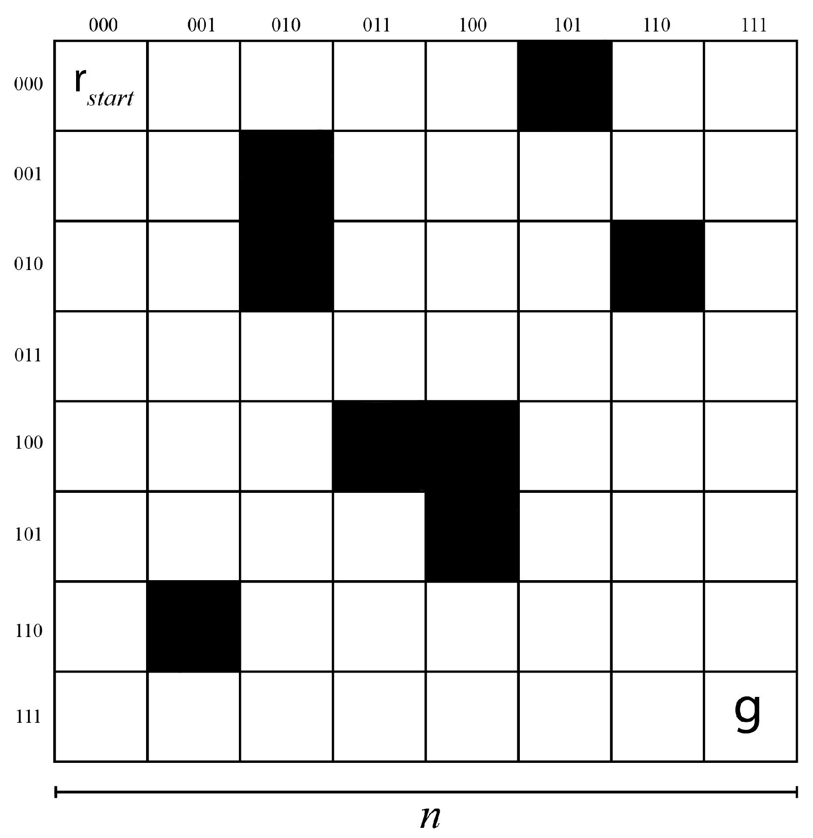
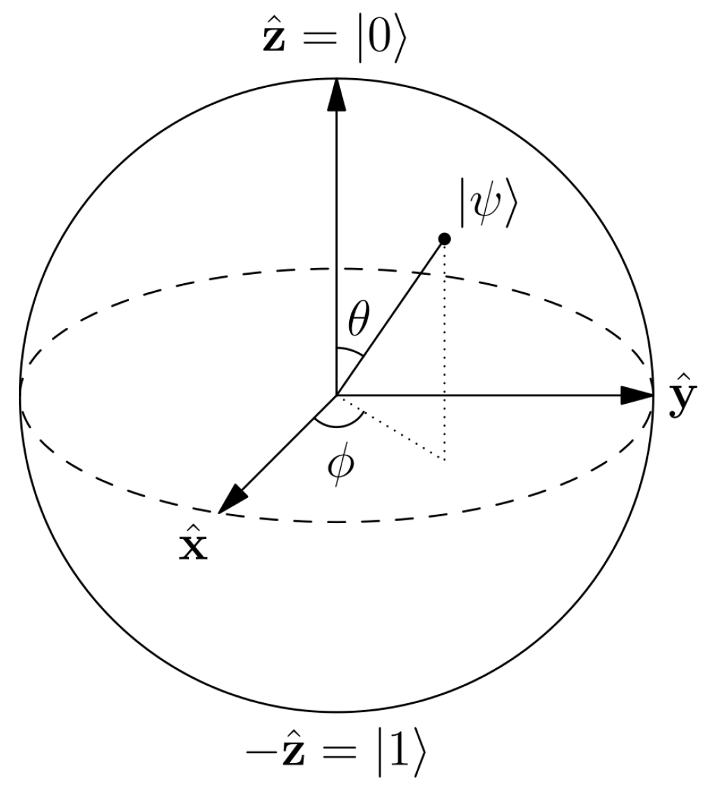
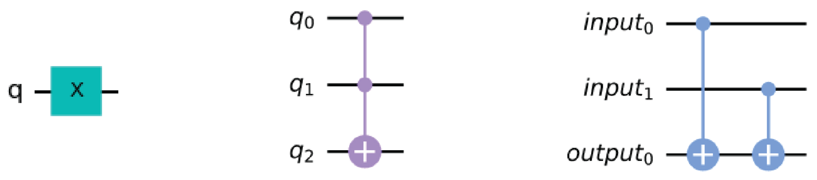
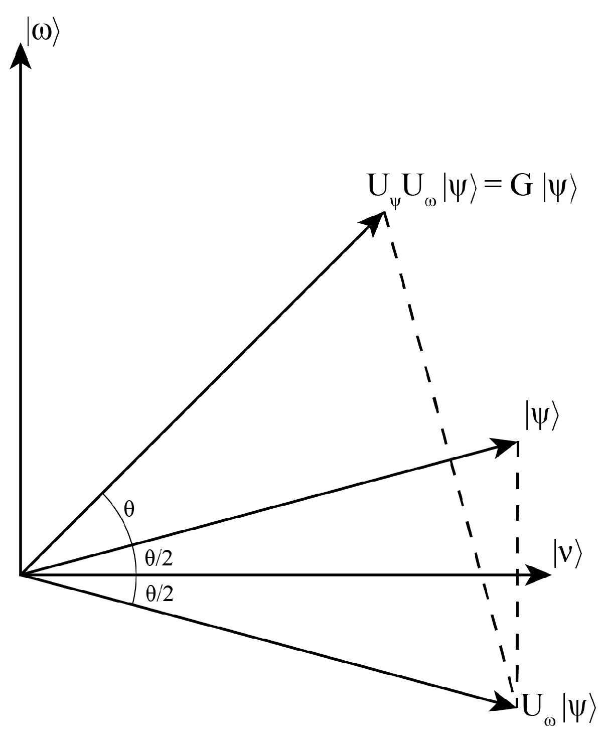
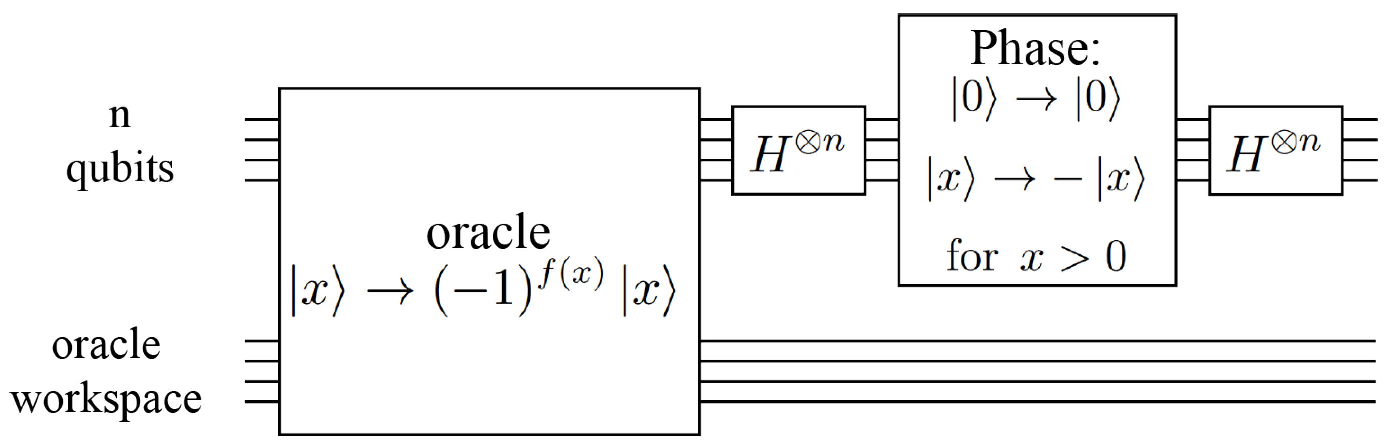
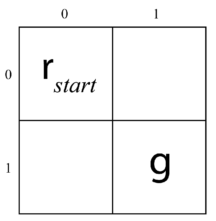
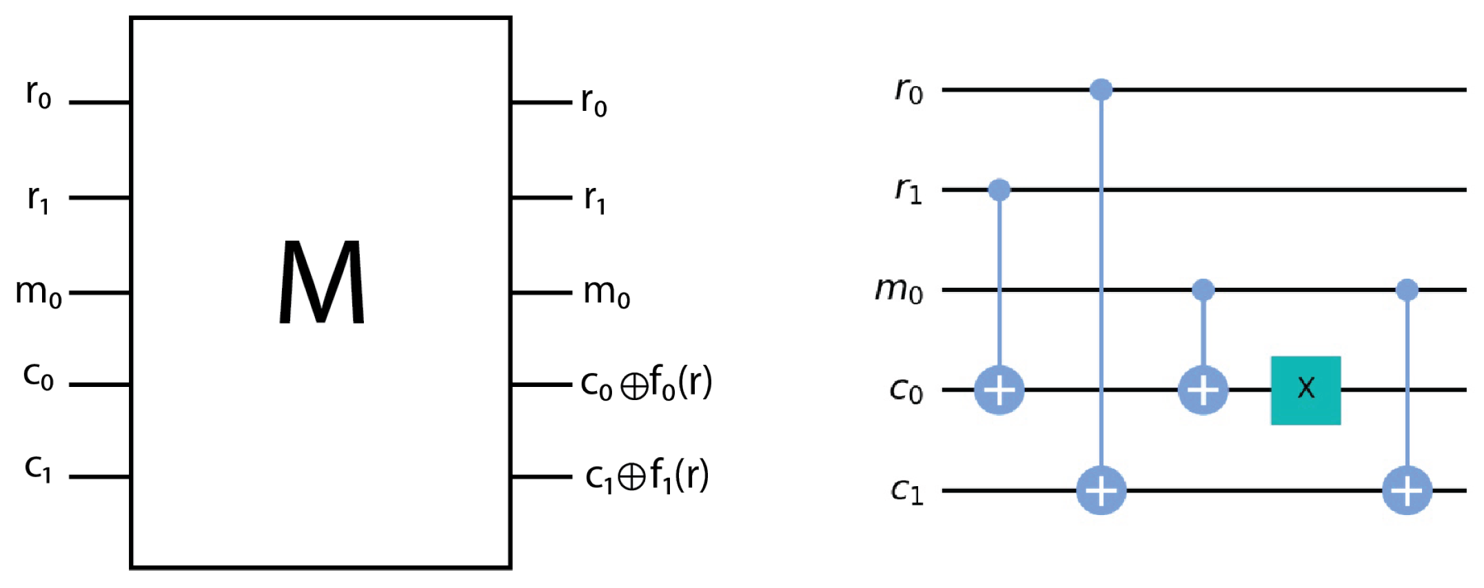
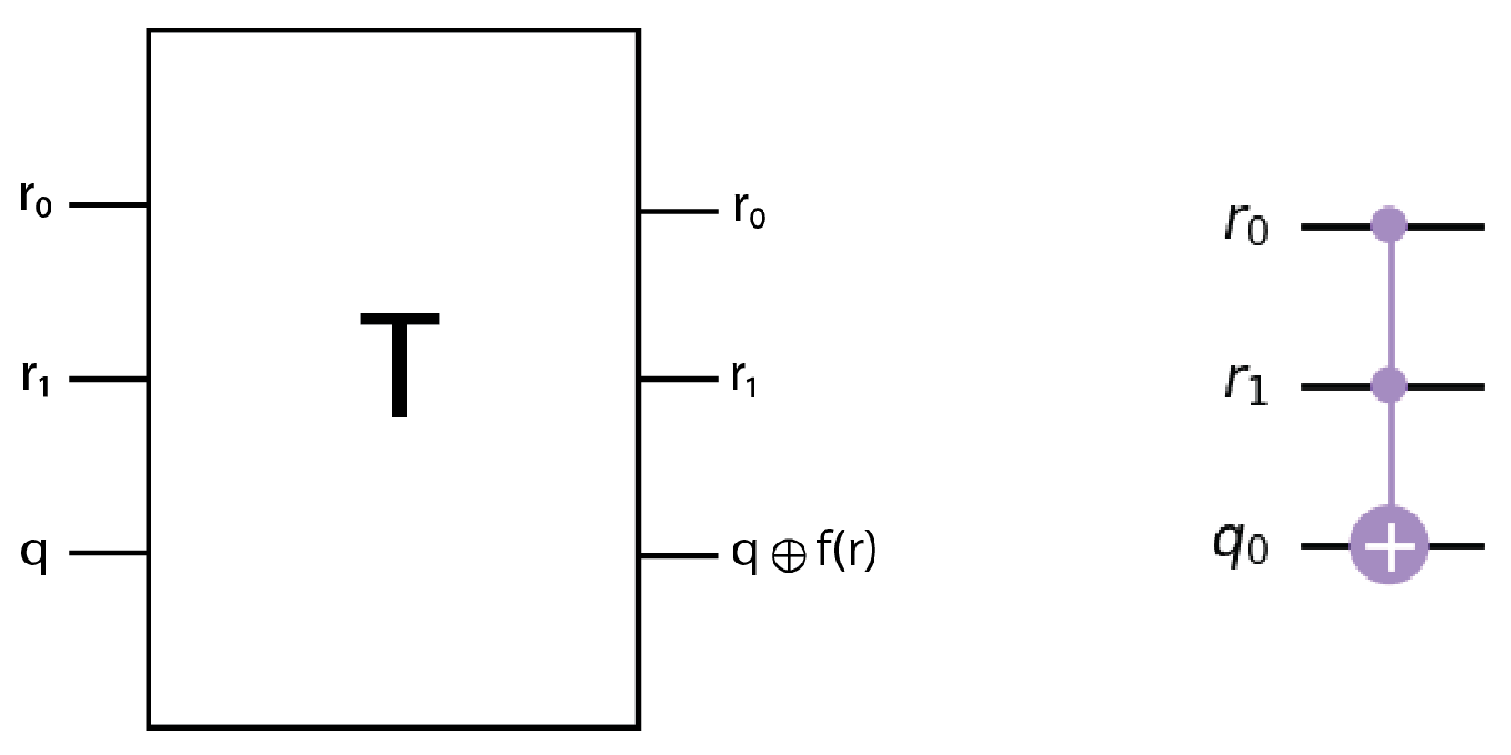
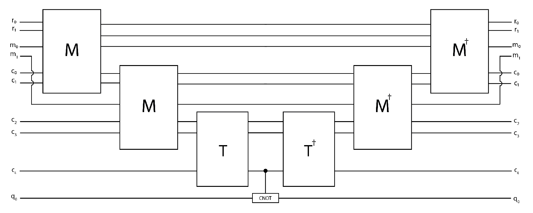
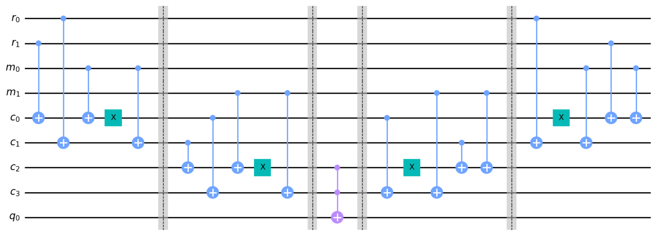
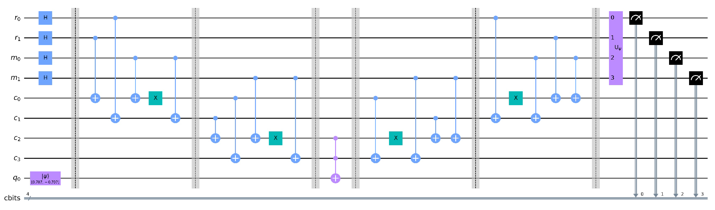
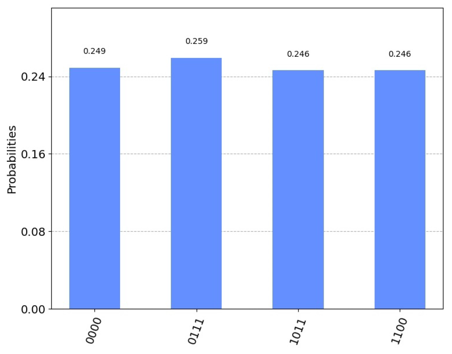
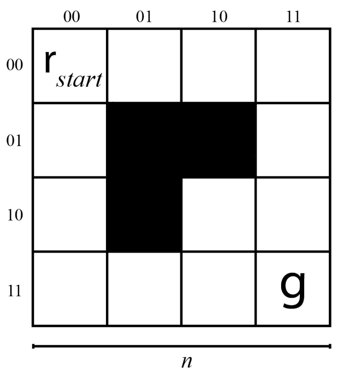
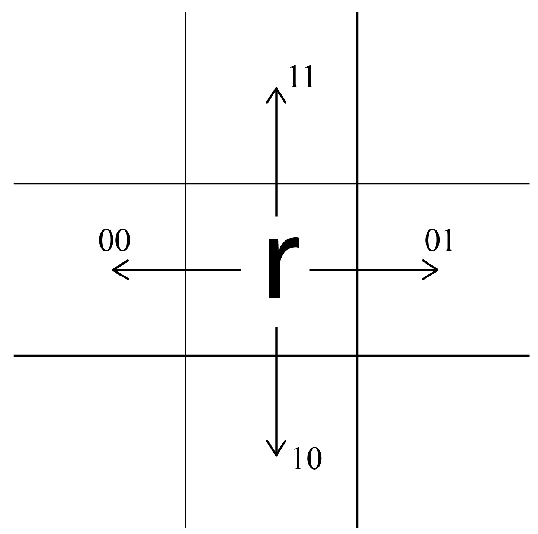
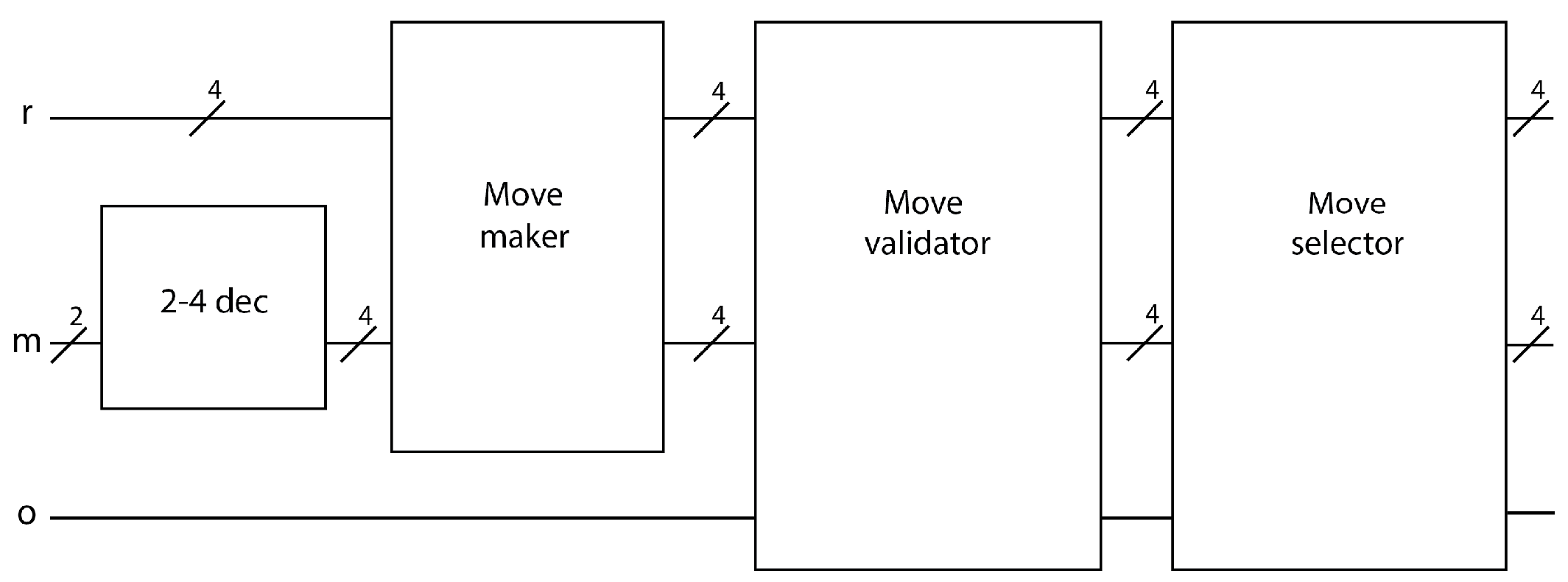
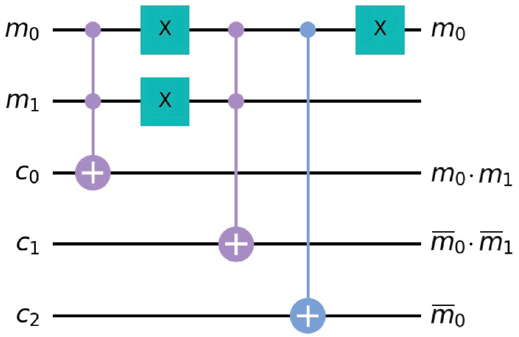
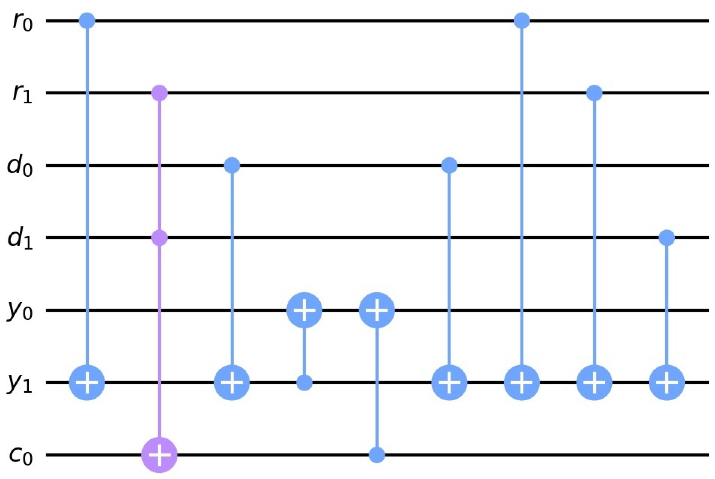
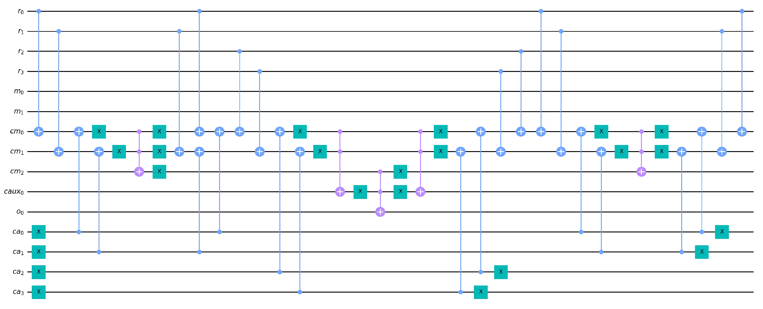
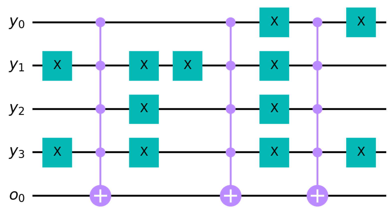
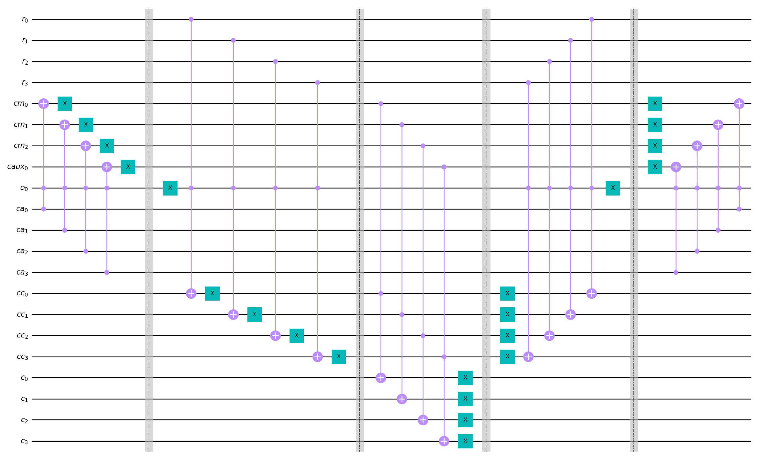
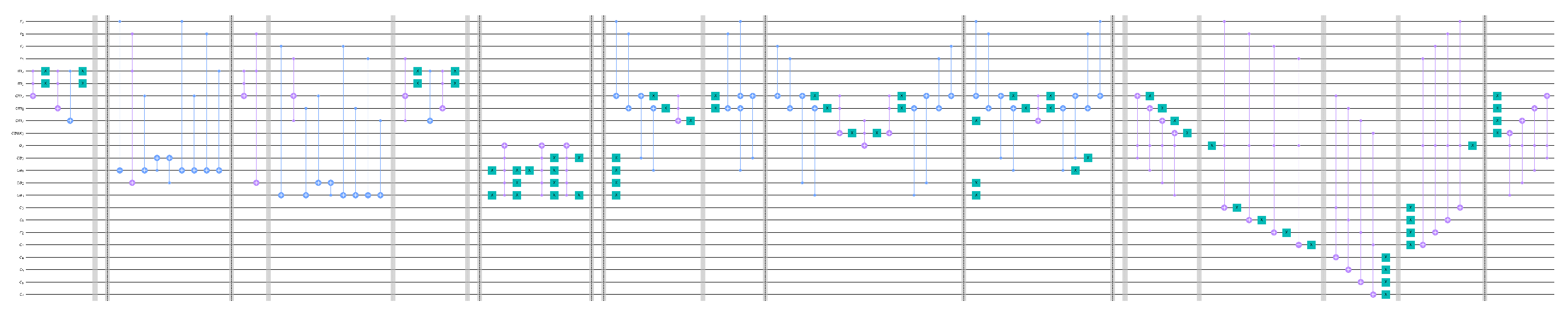
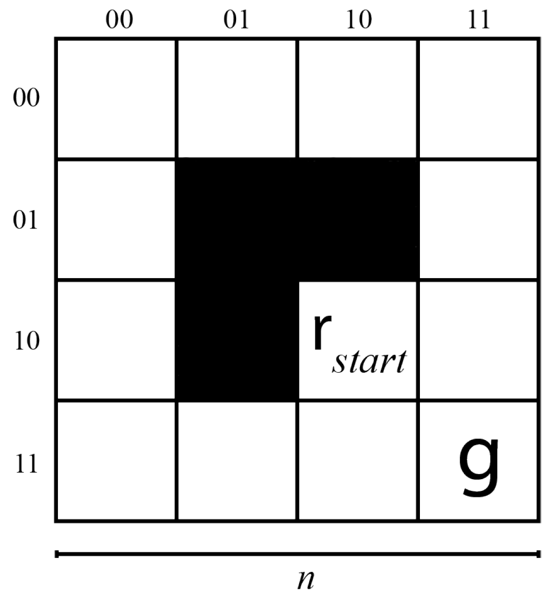
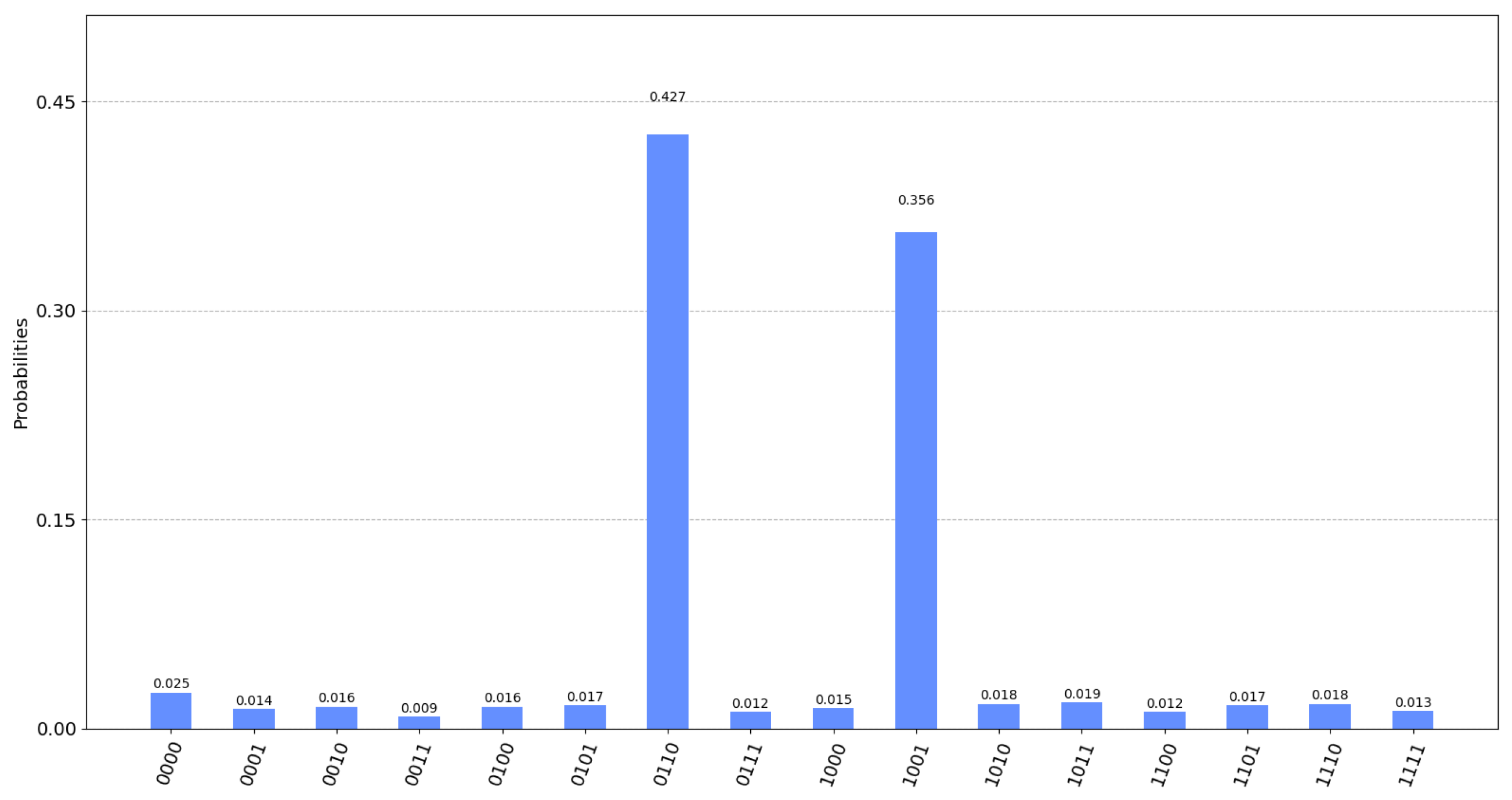
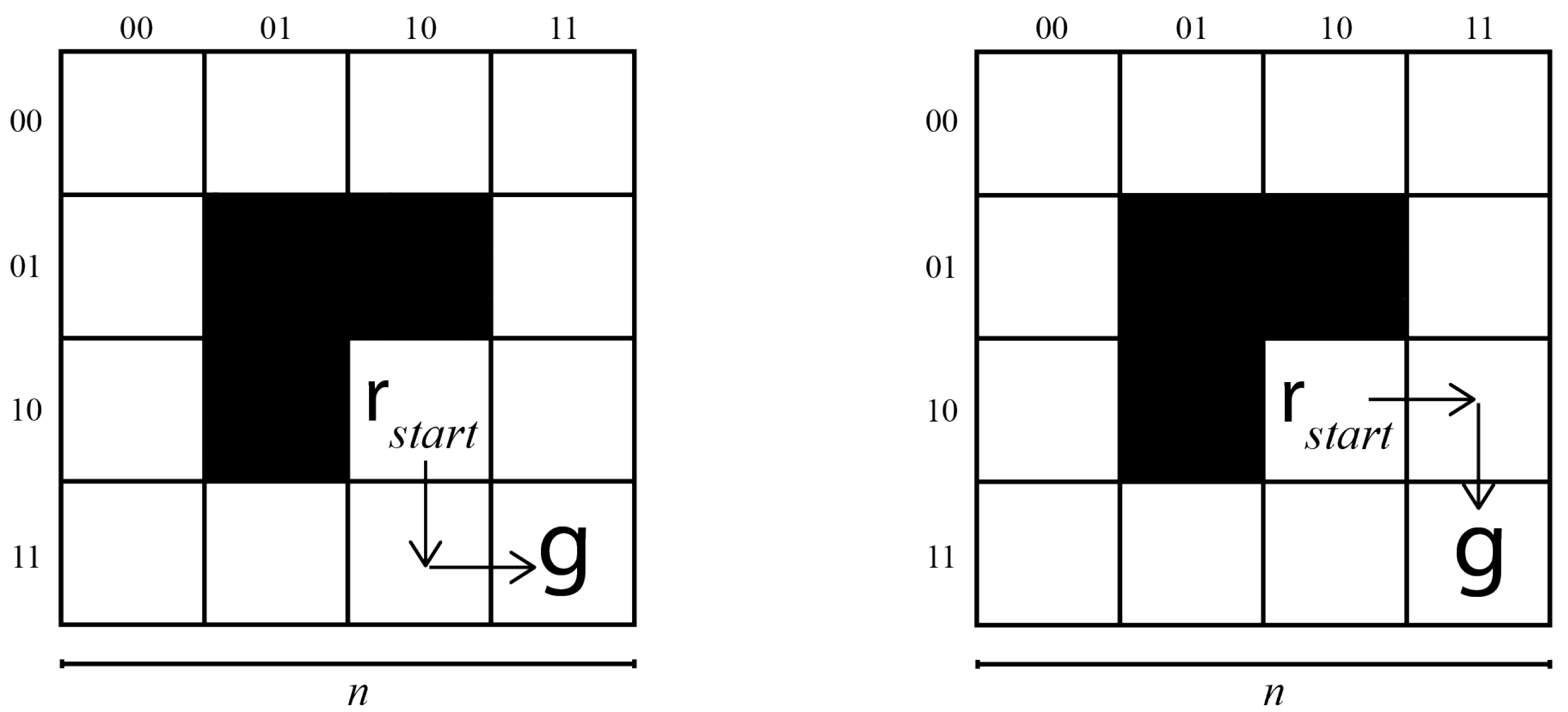
Table 1.
The values of the M block for the position of the robot in the map. and are associated, respectively, with a counter-clockwise and clockwise movement so that for example, if the robot is in and , the new position is .
Table 1.
The values of the M block for the position of the robot in the map. and are associated, respectively, with a counter-clockwise and clockwise movement so that for example, if the robot is in and , the new position is .
| 1 | 0 | 0 | 1 | |
| 0 | 0 | 1 | 1 | |
| 1 | 1 | 0 | 0 | |
| 0 | 1 | 1 | 0 | |
Publisher’s Note: MDPI stays neutral with regard to jurisdictional claims in published maps and institutional affiliations. |
© 2022 by the authors. Licensee MDPI, Basel, Switzerland. This article is an open access article distributed under the terms and conditions of the Creative Commons Attribution (CC BY) license (https://creativecommons.org/licenses/by/4.0/).
Share and Cite
MDPI and ACS Style
Chella, A.; Gaglio, S.; Pilato, G.; Vella, F.; Zammuto, S. A Quantum Planner for Robot Motion. Mathematics 2022, 10, 2475. https://doi.org/10.3390/math10142475
AMA Style
Chella A, Gaglio S, Pilato G, Vella F, Zammuto S. A Quantum Planner for Robot Motion. Mathematics. 2022; 10(14):2475. https://doi.org/10.3390/math10142475
Chicago/Turabian StyleChella, Antonio, Salvatore Gaglio, Giovanni Pilato, Filippo Vella, and Salvatore Zammuto. 2022. "A Quantum Planner for Robot Motion" Mathematics 10, no. 14: 2475. https://doi.org/10.3390/math10142475
Note that from the first issue of 2016, this journal uses article numbers instead of page numbers. See further details here.