Asymmetric Growth of Tumor Spheroids in a Symmetric Environment

Abstract

In this work, we studied the stability of radially symmetric growth in tumor spheroids using a reaction-diffusion model. In this model, nutrient concentration and internal pressure are local variables that implicitly relate the proliferation of cells to the growth of the tumor. The analytical solution of the governing model was presented in an orthonormal spherical harmonic basis. It was shown that the radially symmetric steady-state solution to the growth of tumor spheroids, under symmetric growth conditions, was unstable with respect to small asymmetric perturbations. Such perturbations excited the asymmetric modes of growth, which could grow in time and change the spherical configuration of the tumor. The number of such modes and their rates of growth depended on parameters such as surface tension, external energy and the rate of nutrient consumption. This analysis indicated that the spherical configuration of tumor spheroids, even under experimentally controlled symmetric growth conditions, were naturally unstable. This was confirmed by a comparison between the shapes of in vitro human glioblastoma (hGB) spheroids and the configuration of the first few asymmetric modes predicted by the model.

1. Introduction

Mathematical modeling has great potential in predicting different aspects of tumor progression. The complicated behavior of growing tumors can often be interpreted by understanding the underlying interactions in a mathematical model. In this regard, avascular tumor spheroids have been extensively studied over the past decades [1,2,3,4,5]. The growth of tumor spheroids, in particular, has been mathematically described from different perspectives such as continuum models, discrete (agent-based) models and hybrid (continuum-discrete) models [6]. Continuum models are generally built upon partial differential equations (PDEs) for mass conservation and evolution of the tumor boundary [7,8,9]. In some of these models, the concentration of nutrients defines the cell concentration and type at each point in the tumor body. Indeed, these models implicitly determine the concentration of cells. They can also show acceptable qualitative agreement with experimental data. Furthermore, the literature on mathematical models that explicitly consider the concentration of cells as one of the variables is rapidly growing [10,11,12,13]. In these models, an additional PDE defines the change in the concentration of cells.

Primary invasive tumors emerge from small aggregations of abnormal cells that possess cancerous characteristics, such as high proliferation potential, mainly due to the mutations in their oncogenes, DNA repair genes and/or tumor suppressors [14]. The progression of these tumors starts with the formation of small avascular tumors, followed by a volumetric growth and also the initiation of cell heterogeneity, due to hypoxic/necrotic formation, and finally leads to the formation of large and complex vascular tumors [15]. Among different aspects, asymmetric growth has gained particular attention. Studies have tried to provide insight into why, and how, possible asymmetric configurations may occur during tumor growth [16,17,18]. For instance, the response of spherical tumors to asymmetric perturbations was studied by Byrne and Chaplain [19]. They considered the avascular tumor spheroids as an incompressible fluid where the evolution of the radius depends on the change in internal pressure. The stability of the steady-state solution was then evaluated by examining the excited spherical harmonic modes. They have shown that the growth of invasive tumors evolves according to the unstable modes and that the number of unstable modes increases as the energy required to preserve the tumor structure is reduced. They assumed that the rate of nutrient consumption is constant. This is not a realistic assumption; however, experimental evidence shows that the rate of consumption depends on the nutrient concentration [20]. In addition, the asymptotic stability of the radially symmetric growth of tumor spheroids has been studied in [21,22]. In addition, Li et al. [23], Cristini et al. [24] and Wu et al. [25] carried out numerical simulations of tumor growth in circumstances where a small perturbation can eventually give rise to a radially non-symmetric configuration. The authors investigated the role of a single parameter, such as either nutrient supply or surface tension.

Most of the existing studies either investigated the role of a single parameter in the stability of radially symmetric growth in tumor spheroids, or they lacked an experimental component. In this work, like that of Byrne and Chaplain, we modeled the tumor as a incompressible continuum medium, in which the local proliferation of cells gave rise to a change in internal pressure and, consequently, to growth. However, we relaxed the assumption of a constant consumption rate, adopting instead a concentration-dependent rate, which affected the stability of the steady-state solutions. To observe the behavior of the tumor in response to asymmetric excitation, a small perturbation was introduced to the steady-state solutions. It was seen that increasing the concentration of nutrients, $C_{\infty }$, increased the number of growing asymmetric modes. However, increasing the rate of consumption led to a smaller steady-state radius with a smaller number of growing asymmetric modes. In addition, higher surface tension allowed for a smaller steady-state radius and a smaller number of growing asymmetric modes. We also compared the predicted asymmetric growth with experimental results. The growth of in vitro solid tumor spheroids generated from the glioma cell line (U251 hGB cells) was observed over time. It was seen that spheroids in a roughly symmetric environment lost their spherical configuration due to small natural perturbations from perfect symmetry exerted by their environment.

2. Model Formulation

We adopted a reaction-diffusion model that considered a tumor as an incompressible continuum medium where the proliferation depended on the presence of nutrients. The system of the governing equations is

$$\frac{\partial C(\mathbf{x},t)}{\partial t}={\nabla }^{2}C(\mathbf{x},t)-{\eta }^{2}C(\mathbf{x},t),$$

(1)

$$\frac{\partial P(\mathbf{x},t)}{\partial t}=\mu {\nabla }^{2}P(\mathbf{x},t)+\zeta (C(\mathbf{x},t)-C_d),$$

(2)

$${\mathit{V}}_{\Gamma } · \mathit{n}=-\mu grad P(\mathbf{x},t){|}_{\Gamma } · \mathit{n},$$

(3)

where $C(\mathbf{x},t)$, $P(\mathbf{x},t)$ are the concentrations of nutrients and the internal pressure, respectively, and ${\eta }^{2}C(\mathbf{x},t)$ is the positive rate of nutrient consumption. A constitutive relation analogous to Darcy’s law relates the velocity of cells to the pressure gradient with a constant of proportionality $\mu$ that describes cell motility. The pressure is assumed to be proportional to the cell density, which does not appear explicitly in the equations. However, the pressure production is modulated by the rate of cell proliferation, $\zeta C$, which depends linearly on the concentration of nutrients, and the natural rate of cell death $\zeta C_d$. The tumor boundary is $\Gamma$, ${\mathit{V}}_{\Gamma }$ is the boundary velocity and $n$ is the outward normal. Hence, Equation (3) denotes the rate of growth of the tumor boundary, that is, the normal velocity of its boundary. The boundary of the tumor is a two-phase interface (i.e., cells and nutrients), hence, we impose boundary conditions as

$$C(\mathbf{x},t){|}_{\Gamma }=C_{\infty } \left(1-2\gamma H\right),$$

(4)

$$P(\mathbf{x},t)=P_{\infty },$$

(5)

where (4) is a thermodynamically consistent boundary condition as proposed in [26], $C_{\infty }$ is the nutrient supply, $\gamma$ is the surface tension, H is the mean curvature and $P_{\infty }$ is the external pressure. Equation (4) allows a nutrient concentration jump of $2\gamma H{C}_{\infty }$ across the boundary interface due to the surface tension. It should be noted that the boundary condition (4) couples the system of the governing equations. Next, we present the analytical solution to the governing Equations (1)–(3), subjected to the boundary conditions (4) and (5).

2.1. Analytical Solutions

Spherical coordinates, which are well suited to represent the spherical configuration of tumors, could be used to our advantage. To study the asymmetric instabilities of tumor growth, we first considered the radially symmetric solutions to the governing equation, Equations (1)–(3), and the boundary conditions (4) and (5). The equations can be made more meaningful by the following normalization

$$\overline{C}=\frac{C}{C_d}, {\overline{C}}_{\infty }=\frac{C_{\infty }}{C_d}, \overline{P}=\frac{P}{P_{\infty }}.$$

(6)

Note that in spherical coordinates, the position is $\mathbf{x}=r {\mathit{e}}_{\mathit{r}}(\theta ,\varphi )$ and the Laplace operator ${\nabla }^2$ has the form

$${\nabla }^2=\frac{1}{r^2}\frac{\partial }{\partial r}\left(r^2\frac{\partial }{\partial r}\right)+\frac{1}{r^{2}sin\left(\theta \right)}\frac{\partial }{\partial \theta }\left(sin\left(\theta \right)\frac{\partial }{\partial \theta }\right)+\frac{1}{r^2{sin}^2\left(\theta \right)}\frac{{\partial }^2}{\partial {\varphi }^2},$$

(7)

in the domain $\theta \in [0,\pi ]$ and $\varphi \in [0,2\pi ]$.

Symmetric Steady-State Solutions

For the radially symmetric case, the fields are only a function of r and t, i.e., $C(r,t)$, $P(r,t)$ and the tumor boundary $\Gamma$ is defined by $r=R\left(t\right)$, and its velocity is ${\mathit{V}}_{\Gamma }=V_R{\mathit{e}}_{\mathit{r}}$. Thus, Equations (3) and (4) read

$$V_R=-\mu \frac{\partial P(r,t)}{\partial r}{|}_{r=R\left(t\right)},$$

(8)

$$C(r,t){|}_{r=R\left(t\right)}=C_{\infty } \left(1-2\gamma R^{-1}\left(t\right)\right),$$

(9)

where $V_R$ is the velocity of the tumor boundary and $R\left(t\right)$ is the radius of the tumor. Note that Equation (9) provides a lower bound for $R\left(t\right)$ such that $2\gamma <R\left(t\right)$. To eliminate singularities at $r=0$, we use

$$\frac{\partial C(0,\theta ,\varphi ,t)}{\partial r}=0,$$

(10)

$$\frac{\partial P(0,\theta ,\varphi ,t)}{\partial r}=0.$$

(11)

The solution for the nutrient concentration is

$$\overline{C}(r,t)=\frac{{\overline{C}}_{\infty }(R\left(t\right)-2\gamma )sinh\left(\eta r\right)}{rsinh\left(\eta R\right(t\left)\right)},$$

(12)

and substitution into (2) and (3) yields

$$\frac{\mu P_{\infty }}{\zeta C_d}\frac{\partial \overline{P}}{\partial r}(r,t)=\frac{{\overline{C}}_{\infty }(R\left(t\right)-2\gamma )sinh\left(\eta r\right)}{{\eta }^2{r}^{2}sinh\left(\eta R\left(t\right)\right)}-\frac{{\overline{C}}_{\infty }(R\left(t\right)-2\gamma )cosh\left(\eta r\right)}{\eta rsinh\left(\eta R\right(t\left)\right)}+\frac{r}{3},$$

(13)

$$\frac{1}{\zeta C_d}\frac{dR\left(t\right)}{dt}=\frac{{\overline{C}}_{\infty }\left(R\left(t\right)-2\gamma \right)}{sinh\left(\eta R\right(t\left)\right)} \left(\frac{1}{\eta R\left(t\right)}cosh\left(\eta R\left(t\right)\right)-\frac{1}{{\eta }^{2}R{\left(t\right)}^2}sinh\left(\eta R\left(t\right)\right)\right)-\frac{R\left(t\right)}{3}.$$

(14)

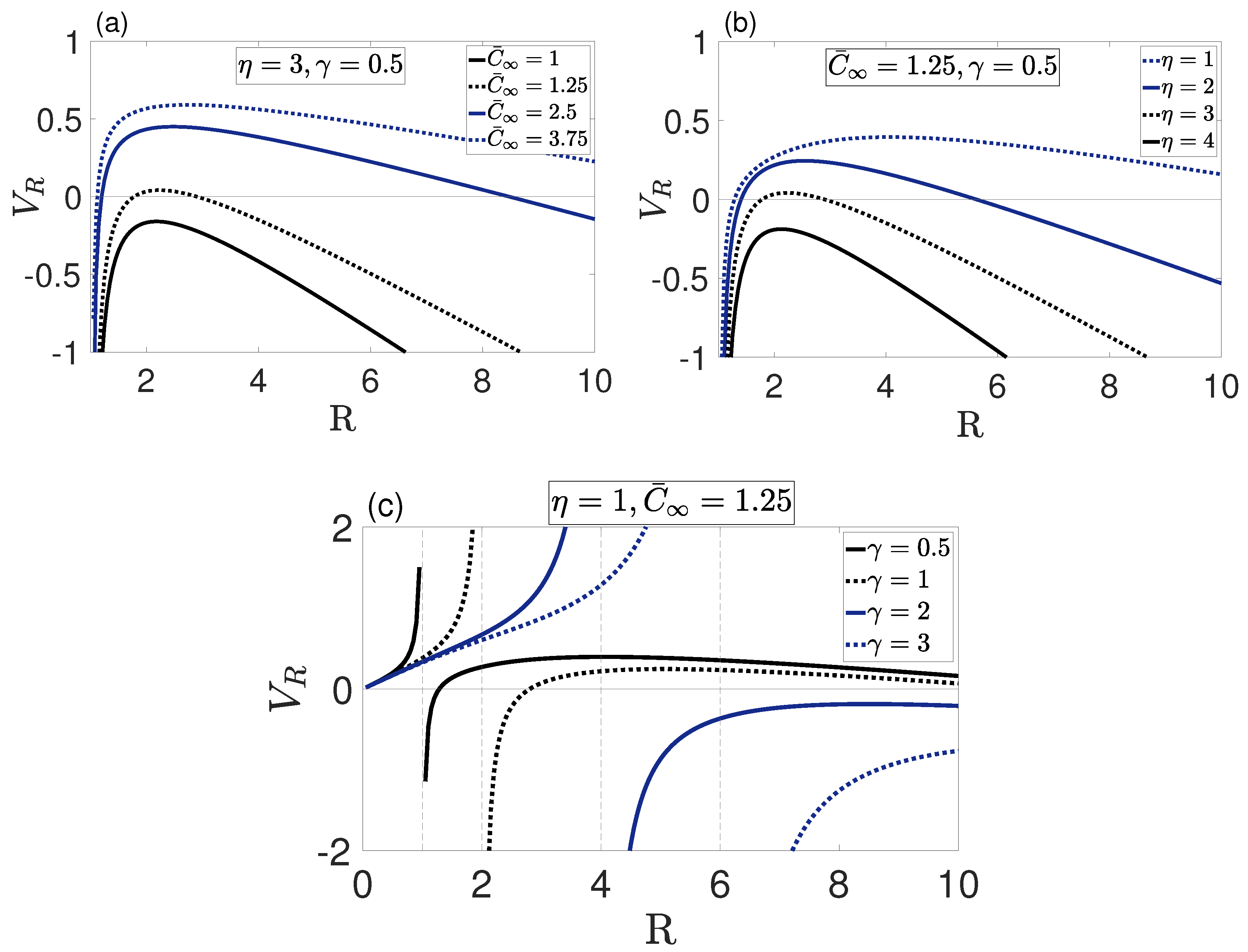
To understand the role of the model parameters, the tumor growth rate $V_R$ was plotted against the tumor radius R for different values of nutrient source $C_{\infty }$, surface tension $\gamma$ and rate of consumption $\eta$.

Figure 1 shows that at most two plausible steady-state solutions, $V_R=0$ existed. The plausible steady-state solutions could be stable for $d{V}_R/dR<0$ or unstable for $d{V}_R/dR>0$. However, in the current context it was necessary for a steady-state solution to be stable. Figure 1a shows that no steady-state solution existed for ${\overline{C}}_{\infty }\le 1$ since the net proliferation was negative due to the limited nutrient supply. Thus, the tumor continuously diminished to zero. For sufficient nutrient supply, ${\overline{C}}_{\infty }\ge 1.25$, two steady-state solutions existed. Similarly, Figure 1b shows that two steady-state solutions existed for the low consumption rate $\eta \le 3$, and no steady-state solution existed for $\eta \ge 4$ due to the insufficient supply of nutrients. It followed that, for a particular $\eta ={\eta }_0$ in the range $(3,4)$, the two solutions coincided into one unstable solution, such that for $0\le \eta <{\eta }_0$ one stable solution existed and for $\eta >{\eta }_0$ no solutions existed. Figure 1c shows that for large surface tension no steady-state solution existed. Recall that $R>2\gamma$, hence the curves where $R<2\gamma$ were not physically admissible. When two plausible steady-state solutions existed, the large radius solution was stable, but the small radius solution was unstable. It was also observed that the radius of the stable steady-state solution increased with increasing ${\overline{C}}_{\infty }$ and decreased with increasing $\eta$ and $\gamma$. It should be noted that only dimensional stability was investigated above; shape stability is yet to be considered. In what follows, we investigated shape instability in the form of asymmetric instability of the radially symmetric steady-state solutions by introducing asymmetric perturbations. We also explored the growth rate of unstable asymmetric modes to obtain an insight into the perturbed configuration of the tumor.

2.2. Instability to Asymmetric Perturbation

A tumor microenvironment can exert external stimuli in various non-symmetric ways. For instance, tumor tissue can apply forces in different directions or cells can be exposed to an asymmetric gradient of chemoattractants, growth factors, etc. In addition, the heterogeneity of the cell population may change the local properties in large tumors and lead to an inhomogeneous structure. Therefore, tumors are susceptible to asymmetric growth. This can be seen in the growth of benign tumors when they eventually lose their close-to-spherical shape. The vast majority of invasive tumors are not spherical [27]. To investigate the stability of the steady-state radially symmetric solution, small time-dependent asymmetric perturbations were introduced as

$$C(r,\theta ,\varphi ,t)=\overline{C}\left(r\right)+ϵ C_p(r,\theta ,\varphi ,t),$$

(15)

$$P(r,\theta ,\varphi ,t)=\overline{P}\left(r\right)+ϵ P_p(r,\theta ,\varphi ,t),$$

(16)

$$R(\theta ,\varphi ,t)=\overline{R}+ϵ R_p(\theta ,\varphi ,t),$$

(17)

where $0<ϵ⩽1$, $\overline{C}\left(r\right),\overline{P}\left(r\right)$ and $\overline{R}$ are the dimensionally stable steady-state radially symmetric solutions of the governing Equations (1)–(3) and $C_p,P_p$ and $R_p$ are the asymmetric perturbations. The substitution of (15) and (16) into (1) and (2) immediately yields the governing equations for $C_p$ and $P_p$, respectively. In order to obtain the equation of $R_p$, first substitute (17) into (3), which yields

$$\frac{\partial }{\partial t}\left(\overline{R}+ϵ R_p\right)=-\mu \frac{\partial }{\partial r}\left(\overline{P}+ϵ P_p\right){|}_{r=\overline{R}+ϵ R_p},$$

(18)

and then utilize the Taylor series of (16) about $\overline{R}$ in the form

$$\frac{\partial }{\partial r}\left(\overline{P}+ϵ P_p\right){|}_{r=\overline{R}+ϵR_p}=\frac{\partial \overline{P}}{\partial r}{|}_{r=\overline{R}}+ϵ\frac{\partial P_p}{\partial r}{|}_{r=\overline{R}}+ϵR_p\frac{{\partial }^2\overline{P}}{{\partial }^{2}r}{|}_{r=\overline{R}}+O\left({ϵ}^2\right).$$

(19)

Finally, substitution of (19) into (18) yields the governing equation for $C_p$. The system of governing equations of the perturbations $C_p$, $P_p$ and $R_p$ reads

$${\nabla }^2{C}_p-{\eta }^2{C}_p=0,$$

(20)

$$\mu {\nabla }^2{P}_p+\zeta C_p=0,$$

(21)

$$\frac{\partial R_p}{\partial t}=-\mu \left(\frac{\partial P_p}{\partial r}+R_p \frac{{\partial }^2\overline{P}}{\partial r^2}\right){|}_{r=\overline{R}}.$$

(22)

Similarly, substitution of the perturbations into (4) and (5) yields the perturbed boundary conditions

$$C_p{|}_{r=\overline{R}}=\frac{\gamma C_{\infty }}{{\overline{R}}^2} \left[2R_p+\frac{1}{r^{2}sin\left(\theta \right)}\frac{\partial }{\partial \theta }\left(sin\left(\theta \right)\frac{\partial R_p}{\partial \theta }\right)+\frac{1}{r^2{sin}^2\left(\theta \right)}\frac{{\partial }^2{R}_p}{\partial {\varphi }^2}\right]-R_p\frac{\partial C}{\partial r}{|}_{r=\overline{R}},$$

(23)

$$P_p{|}_{r=\overline{R}}=-R_p \frac{\partial P}{\partial r}{|}_{r=\overline{R}}.$$

(24)

Also, the following conditions can be simply inferred from (10) and (11)

$$\frac{\partial C_p}{\partial r}{|}_{r=0}=0,$$

(25)

$$\frac{\partial P_p}{\partial r}{|}_{r=0}=0.$$

(26)

Separation of variables $C_p\left(r,\theta ,\varphi \right)=R\left(r\right)\Theta \left(\theta \right)\Phi \left(\varphi \right)$ is used to solve Equation (20). Substitution gives the following equations for the polar and azimuthal angles

$$\frac{1}{\Phi \left(\varphi \right)}\frac{d^2\Phi \left(\varphi \right)}{d{\varphi }^2}=-m^2 \to \Phi \left(\varphi \right)=e^{im\varphi },$$

(27)

$$\frac{d}{dx}\left((1-x^2)\frac{d\Theta \left(x\right)}{dx}\right)+\left(l(l+1)-\frac{m^2}{1-x^2}\right)\Theta \left(x\right)=0 \to \Theta \left(x\right)=P_l^m\left(x\right),$$

(28)

where m is an integer, $x=cos\theta$ and $P_l^m\left(x\right)=\frac{1}{2^l l!}{(1-x^2)}^{\frac{m}{2}}\frac{d^{l+m}}{d{x}^{l+m}}{(x^2-1)}^l$ are the Legendre polynomials. Combining $\Theta \left(\theta \right)$ and $\Phi \left(\varphi \right)$ forms the spherical harmonics

$$Y_l^m(\Theta ,\varphi )={\chi }_{lm} P_l^m\left(x\right) e^{im\varphi },$$

(29)

where the coefficients ${\chi }_{lm}\left(t\right)$ are determined by the boundary conditions. The equation for the radial component of $C_p\left(r,\theta ,\varphi \right)$ reads

$$r^2\frac{d^{2}z}{d{r}^2}+r\frac{dz}{dr}-\left({\eta }^2{r}^2+{\left(l+\frac{1}{2}\right)}^2\right)z=0,$$

(30)

where $z=R\left(r\right){\left(\eta r\right)}^{\frac{1}{2}}$. The known solutions to Equation (30) are the modified spherical Bessel functions of the first kind, $R\left(r\right)=i_l^{\left(1\right)}\left(\eta r\right)$, where $i_l^{\left(1\right)}\left(\eta r\right)=\sqrt{\left(\frac{\pi }{2r}\right)} I_{l+\frac{1}{2}}\left(\eta r\right)$; $I_{l+\frac{1}{2}}$ is Bessel’s function of the first kind. Gathering all components of the solution yields (note that here we used $i_l^{{\left(1\right)}^{\prime }}\left(r\right)=i_{l+1}^{\left(1\right)}\left(\eta R\left(t\right)\right)+\frac{l}{\eta R\left(t\right)}{i}_l^{\left(1\right)}\left(\eta R\left(t\right)\right))$,

$$C_p\left(R\left(r\right),\Theta (\theta \right),\Phi \left(\varphi \right))=\sum _{l\ge 0}\sum _{\left|m\right|\le l}{\chi }_{lm}\left(t\right) i_l^{\left(1\right)}\left(\eta r\right) Y_l^m(\theta ,\varphi ).$$

(31)

To solve for the pressure, we multiply (20) by $\frac{s}{{\eta }^2}$ and add it to (21) to obtain

$${\nabla }^2\left(P_p+\frac{s}{{\eta }^2\mu }{C}_p\right)=0.$$

It follows that the known solution is

$$P_p+\frac{\zeta }{{\eta }^2\mu }{C}_p=\sum _{l\ge 0}\sum _{\left|m\right|\le l}{\Pi }_{lm}\left(t\right)r^l Y_l^m(\theta ,\varphi ),$$

which by (31) yields the final solution in the form

$$P_p\left(R\left(r\right),\Theta (\theta \right),\Phi \left(\varphi \right))=\sum _{l\ge 0}\sum _{\left|m\right|\le l}\left({\Pi }_{lm}\left(t\right)r^l-\frac{\zeta }{{\eta }^2\mu }{\chi }_{lm}\left(t\right) i_l^{\left(1\right)}\left(\eta r\right)\right) Y_l^m(\theta ,\varphi ),$$

(32)

where the coefficients ${\Pi }_{lm}\left(t\right)$ are determined by the boundary conditions. From (25) and (26), we infer that

$${\chi }_{1m}\left(t\right)=0 \mathrm{and} {\Pi }_{1m}\left(t\right)=0,$$

and from (24), we find ${\rho }_{1m}\left(t\right)=0$. For $l\ne 1$ we have

$$\begin{array}{cc}\hfill {\chi }_{lm}\left(t\right) i_l^{\left(1\right)}\left(\frac{\eta R\left(t\right)}{C_d}\right)=& \left[\frac{\gamma {\overline{C}}_{\infty }}{R^2}(2-l(l+1))-\frac{\partial \overline{C}}{\partial r}\left(R\left(t\right)\right)\right]{\rho }_{lm}\left(t\right)\hfill \\ \hfill =& \left(-l(l+1)\frac{\gamma }{R{\left(t\right)}^2}-\left(1-\frac{2\gamma }{R\left(t\right)}\right)\eta coth\left(\eta R\left(t\right)\right)+\frac{1}{R\left(t\right)}\right){\overline{C}}_{\infty }{\rho }_{lm}\left(t\right) ,\hfill \end{array}$$

(33)

and by (32)

$$\begin{array}{cc}\hfill & \frac{1}{C_d{P}_{\infty }}\left({\Pi }_{lm}\left(t\right)R{\left(t\right)}^l-\frac{\zeta }{{\eta }^2\mu }{\chi }_{lm}\left(t\right) i_l^{\left(1\right)}\left(\eta R\left(t\right)\right)\right)=-\frac{\partial \overline{P}}{\partial r}\left(R\left(t\right)\right) \frac{{\rho }_{lm}\left(t\right)}{C_d}\hfill \\ \hfill & =\left(-\frac{{\overline{C}}_{\infty }}{{\eta }^2}\left(\frac{1}{R\left(t\right)}-\frac{2\gamma }{R{\left(t\right)}^2}\right)+\frac{{\overline{C}}_{\infty }}{\eta }\left(1-\frac{2\gamma }{R\left(t\right)}\right)coth\left(\eta R\left(t\right)\right)-\frac{R\left(t\right)}{3}\right)\frac{\zeta }{P_{\infty }\mu }{\rho }_{lm}\left(t\right).\hfill \end{array}$$

(34)

Hence, substitution of (33) into (34) yields

$$\begin{array}{c}\hfill \frac{\mu }{C_d\zeta }{\Pi }_{lm}\left(t\right)R{\left(t\right)}^l=\left((1-l)(l+2)\frac{\gamma {\overline{C}}_{\infty }}{{\eta }^{2}R{\left(t\right)}^2}-\frac{R\left(t\right)}{3}\right){\rho }_{lm}\left(t\right).\end{array}$$

(35)

By writing the perturbed radius in an orthonormal spherical basis,

$$R_p\left(t\right)=\sum _{l\ge 0}\sum _{\left|m\right|\le l}{\rho }_{lm}\left(t\right) Y_l^m(\theta ,\varphi ),$$

(36)

and implementing (22), we conclude that $\frac{d{\rho }_{1m}}{dt}\left(t\right)=0$ and for $l\ne 1$

$$\begin{array}{cc}\hfill \frac{1}{C_d\zeta {\rho }_{lm}\left(t\right)}\frac{d{\rho }_{lm}\left(t\right)}{dt}=& -\frac{\mu }{C_d}\left(l {\Pi }_{lm}\left(t\right) l R{\left(t\right)}^{l-1}-\frac{\zeta }{\mu \eta }{\chi }_{lm}\left(t\right) i_l^{{\left(1\right)}^{\prime }}\left(\eta R\left(t\right)\right)+\frac{{\partial }^{2}P}{\partial r^2}\left(R\left(t\right)\right)\right)\hfill \\ \hfill =& -l\frac{\mu }{C_d\zeta }{\Pi }_{lm}\left(t\right)R{\left(t\right)}^{l-1}+\frac{1}{C_d\eta }{\chi }_{lm}\left(t\right) \left(i_{l+1}^{\left(1\right)}\left(\eta R\left(t\right)\right)+\frac{l}{\eta R\left(t\right)}{i}_l^{\left(1\right)}\left(\eta R\left(t\right)\right)\right)\hfill \\ \hfill & -\frac{2{\overline{C}}_{\infty }(R\left(t\right)-2\gamma )coth\left(\eta R\left(t\right)\right)}{\eta R{\left(t\right)}^2}+\frac{2{\overline{C}}_{\infty }(R\left(t\right)-2\gamma )}{{\eta }^{2}R{\left(t\right)}^3}+\frac{{\overline{C}}_{\infty }(R\left(t\right)-2\gamma )}{R\left(t\right)}-\frac{1}{3}\hfill \\ \hfill =& -\frac{l}{R\left(t\right)}\frac{\mu }{C_d\zeta }\left({\Pi }_{lm}\left(t\right)R{\left(t\right)}^l-\frac{1}{\eta }{\chi }_{lm}\left(t\right) i_l^{\left(1\right)}\left(\eta R\left(t\right)\right)\right)+\frac{1}{C_d\eta }{\chi }_{lm}\left(t\right) i_{l+1}^{\left(1\right)}\left(\eta R\left(t\right)\right)\hfill \\ \hfill & -\frac{2{\overline{C}}_{\infty }(R\left(t\right)-2\gamma )coth\left(\eta R\left(t\right)\right)}{\eta R{\left(t\right)}^2}+\frac{2{\overline{C}}_{\infty }(R\left(t\right)-2\gamma )}{{\eta }^{2}R{\left(t\right)}^3}+\frac{{\overline{C}}_{\infty }(R\left(t\right)-2\gamma )}{R\left(t\right)}-\frac{1}{3}\hfill \\ \hfill =& -\frac{l}{R\left(t\right)}\left(-\frac{{\overline{C}}_{\infty }}{{\eta }^2}\left(\frac{1}{R\left(t\right)}-\frac{2\gamma }{R{\left(t\right)}^2}\right)+\frac{{\overline{C}}_{\infty }}{\eta }\left(1-\frac{2\gamma }{R\left(t\right)}\right)coth\left(\eta R\left(t\right)\right)-\frac{R\left(t\right)}{3}\right)\hfill \\ \hfill & -\frac{2{\overline{C}}_{\infty }(R\left(t\right)-2\gamma )coth\left(\eta R\left(t\right)\right)}{\eta R{\left(t\right)}^2}+\frac{2{\overline{C}}_{\infty }(R\left(t\right)-2\gamma )}{{\eta }^{2}R{\left(t\right)}^3}+\frac{{\overline{C}}_{\infty }(R\left(t\right)-2\gamma )}{R\left(t\right)}-\frac{1}{3}\hfill \\ \hfill & +\frac{1}{C_d\eta }{\chi }_{lm}\left(t\right) i_{l+1}^{\left(1\right)}\left(\eta R\left(t\right)\right) .\hfill \end{array}$$

Finally, from (33) we obtain

$$\begin{array}{cc}\hfill \frac{1}{C_d\zeta {\rho }_{lm}\left(t\right)}\frac{d{\rho }_{lm}\left(t\right)}{dt}=& (l+2)\frac{{\overline{C}}_{\infty }(R\left(t\right)-2\gamma )}{{\eta }^{2}R{\left(t\right)}^3}-(l+2)\frac{{\overline{C}}_{\infty }(R\left(t\right)-2\gamma )coth\left(\eta R\left(t\right)\right)}{\eta R{\left(t\right)}^2}\hfill \\ \hfill & +\frac{{\overline{C}}_{\infty }(R\left(t\right)-2\gamma )}{R\left(t\right)}+(l-1)\frac{1}{3}\hfill \\ \hfill & +\left(-l(l+1)\frac{\gamma {\overline{C}}_{\infty }}{R^2}-{\overline{C}}_{\infty }\left(1-\frac{2\gamma }{R\left(t\right)}\right)\eta coth\left(\eta R\left(t\right)\right)+\frac{{\overline{C}}_{\infty }}{R\left(t\right)}\right)\frac{i_{l+1}^{\left(1\right)}\left(\eta R\left(t\right)\right)}{\lambda i_l^{\left(1\right)}\left(\eta R\left(t\right)\right)} .\hfill \end{array}$$

(37)

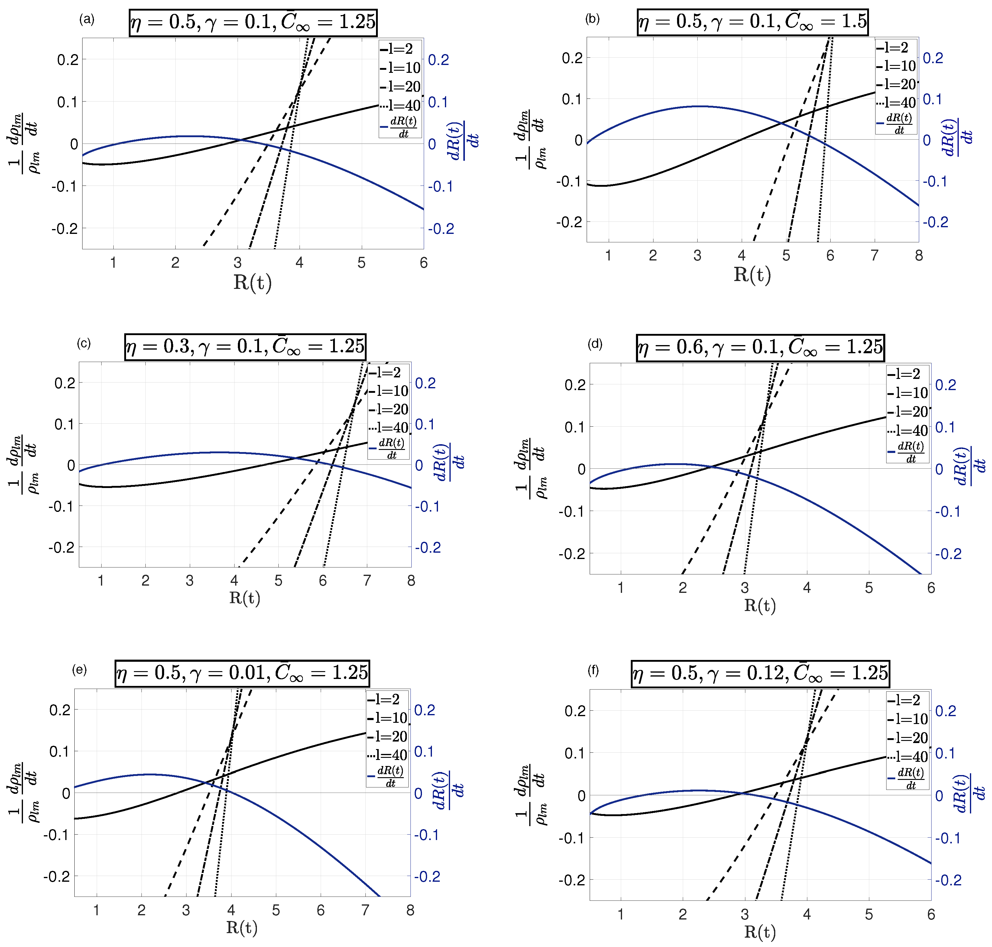
Equation (37) describes the growth of asymmetric modes ${\rho }_{lm}\left(t\right)$ in time, which depends on both system parameters $\{C_{\infty },C_d,\gamma ,\eta \}$ and the system variable $R\left(t\right)$. These modes can be either excited or damped for various ranges of $R\left(t\right)$. In order to find these ranges, the evolution equation in (37) was plotted against $R\left(t\right)$ for particular choices of system parameters in Figure 2. Each curve corresponded to a particular asymmetric mode number. The rate of growth $dR\left(t\right)/dt$ was also plotted to indicate the steady-state radially symmetric solutions. As discussed in Section 2.1, there were at most two steady-state solutions, $0<R_1<R_2$, depicted in the figure, identified by $dR/dt=0$; however, only $R_2$ was dimensionally stable. Therefore, we carried out asymmetric stability analysis only for $R_2$.

For a given $R_2$, high mode numbers were stable, but low mode numbers were unstable as can be seen in Figure 2. Note that changing the system parameters changed the number of stable and unstable modes. As can be seen in Figure 2a,b, increasing the concentration of nutrients $C_{\infty }$ increased the number of growing asymmetric modes. This was directly related to the tumor’s access to nutrients, which increased tumor activity and proliferation, which in turn enabled them to adopt a new homeostatic equilibrium and become invasive. This allowed the tumor to evolve from a spherical shape, which was energy-wise preferred, and grow along asymmetric modes, called invasion modes. Therefore, a higher concentration of nutrients enabled a tumor to gain invasion modes. On the other hand, as depicted in Figure 2c,d, increasing the rate of consumption led to a smaller steady-state radius with a smaller number of invasion asymmetric modes. The same behavior can be seen for the change in surface tension $\left(\gamma \right)$ in Figure 2e,f. Higher surface tension allowed for a smaller steady-state radius and a smaller number of growing asymmetric modes.

2.3. Growing Asymmetric Modes

To achieve insight into the perturbed configuration of the tumor, it was important to find the fastest growing mode, i.e., the dominant mode number $l_d$. Such mode(s) could determine the long-term change in the shape of the tumor. In addition, the surface tension $\gamma$ could stabilize the growth of this mode. Therefore, we centered our focus on the variation of $l_d$ for different values of $\gamma$, in close proximity to the steady-state solution $R_2\left(t\right)$. The steady-state solution of (14), $dR/dt=0$, takes the form

$$\frac{{\overline{C}}_{\infty }(R\left(t\right)-2\gamma )}{{\eta }^{2}R{\left(t\right)}^2}-\frac{{\overline{C}}_{\infty }(R\left(t\right)-2\gamma )}{\eta R\left(t\right)}coth\left(\eta R\left(t\right)\right)+\frac{R\left(t\right)}{3}=0.$$

Substitution of this into (37) gives

$$\begin{array}{cc}\hfill \frac{1}{C_d\zeta {\rho }_{lm}\left(t\right)}\frac{d{\rho }_{lm}\left(t\right)}{dt}& =\frac{{\overline{C}}_{\infty }(R-2\gamma )}{R\left(t\right)}\hfill \\ \hfill & +\left((1-l)(l+2)\frac{\gamma {\overline{C}}_{\infty }}{R^2}+\frac{{\eta }^{2}R}{3}\right)\frac{i_{l+1}^{\left(1\right)}\left(\eta R\right)}{\eta i_l^{\left(1\right)}\left(\eta R\right)}-1 .\hfill \end{array}$$

(38)

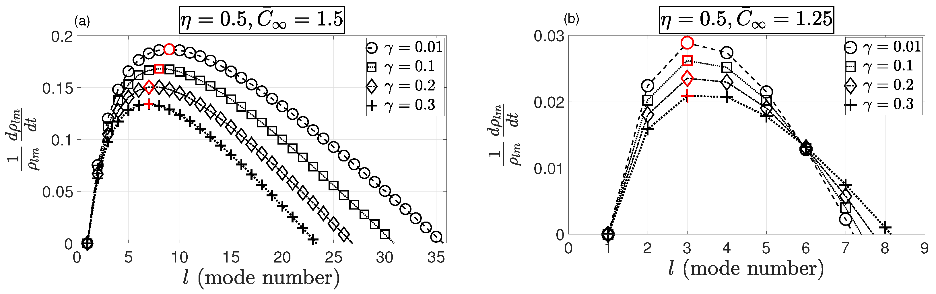
To better understand the role of the surface tension, $\gamma$, given a particular choice of system parameters $\{C_{\infty },C_d,\eta \}$, Equation (37) can be expressed as in Equation (38) as a function only of l and $\gamma$. Figure 3 shows the positive rate of growth of asymmetric modes. Modes with a negative rate of growth (damped modes) were neglected. Mode numbers that had the maximum rate of growth (maximal modes) are marked in red. It can be seen that for ${\overline{C}}_{\infty }=1.5$, by increasing the surface tension the dominant mode dropped from $l=9$ to $l=7$; however, it had a fixed value of $l=3$ for ${\overline{C}}_{\infty }=1.2$. This behavior could be interpreted as the role of nutrients and surface tension on tumor invasiveness, that is, a higher concentration of nutrient source maximized the growth of a higher asymmetric mode number, which dropped to a lower mode number by increasing the surface tension.

3. Asymmetric Configuration

The progression of tumors starts with the formation of small symmetric-shaped avascular tumors (spherical configuration) and proceeds with their volumetric growth. However, a tumor microenvironment can exert external stimuli that trigger asymmetric growth and, therefore, tumors lose their symmetric shape and acquire an asymmetric configuration. Here, we present an instability analysis of such responses as associated with tumor invasion modes. We considered asymmetric radius perturbation (17) in terms of a spherical harmonic basis, which has the form of (36). The perturbed axisymmetric radius is a superposition of infinitely many modes. However, only the growing modes, and particularly the maximal mode, eventually dominate the tumor configuration. The total radius is

$$R_t(\theta ,\varphi ,t)=\overline{R}+ϵ \sum _{l\ge 0}\sum _{\left|m\right|\le l}{\rho }_{lm}\left(t\right) Y_l^m(\theta ,\varphi ),$$

(39)

where $\overline{R}$ is the steady-state radius. Integration of (38) gives the evolution of coefficients

$${\rho }_{lm}\left(t\right)={\rho }_{lm}^{0}exp\left(\frac{\zeta }{C_d}\left(\frac{{\overline{C}}_{\infty }(R-2\gamma )}{R}+\left((1-l)(l+2)\frac{\gamma {\overline{C}}_{\infty }}{R^2}+\frac{{\eta }^{2}R}{3}\right)\frac{i_{l+1}^{\left(1\right)}\left(\lambda R\right)}{\eta i_l^{\left(1\right)}\left(\eta R\right)}-1\right)t\right),$$

(40)

where ${\rho }_{lm}^0$ are the coefficients corresponding to the initial condition $R_{p_0}$, i.e.,

$$R_{p_0}(\theta ,\varphi )=\sum _{l\ge 0}\sum _{\left|m\right|\le l}{\rho }_{lm}^0 Y_l^m(\theta ,\varphi ).$$

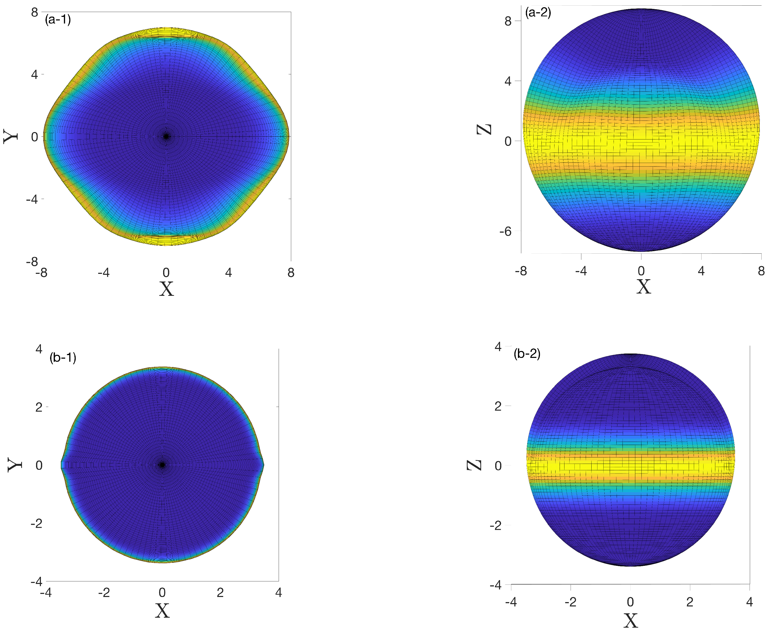
Figure 4 depicts the three-dimensional configurations of the tumor (39) and (40) after sufficient time when only the growing modes were observable. For the two choices of parameters used in Figure 2a,b, i.e., $\{{\overline{C}}_{\infty }=1.25,\eta =0.5,\gamma =0.1,\overline{R}=3.37\}$ and $\{{\overline{C}}_{\infty }=1.5,\eta =0.5,\gamma =0.1,\overline{R}=5.69\}$, the corresponding unstable modes were $l=\{0,2,3,...,7\}$ and $l=\{0,2,3,...,30\}$, respectively. Implementing these parameters and the unstable modes in (39), perturbed radii were obtained to plot the asymmetric configurations.

4. Results and Discussion

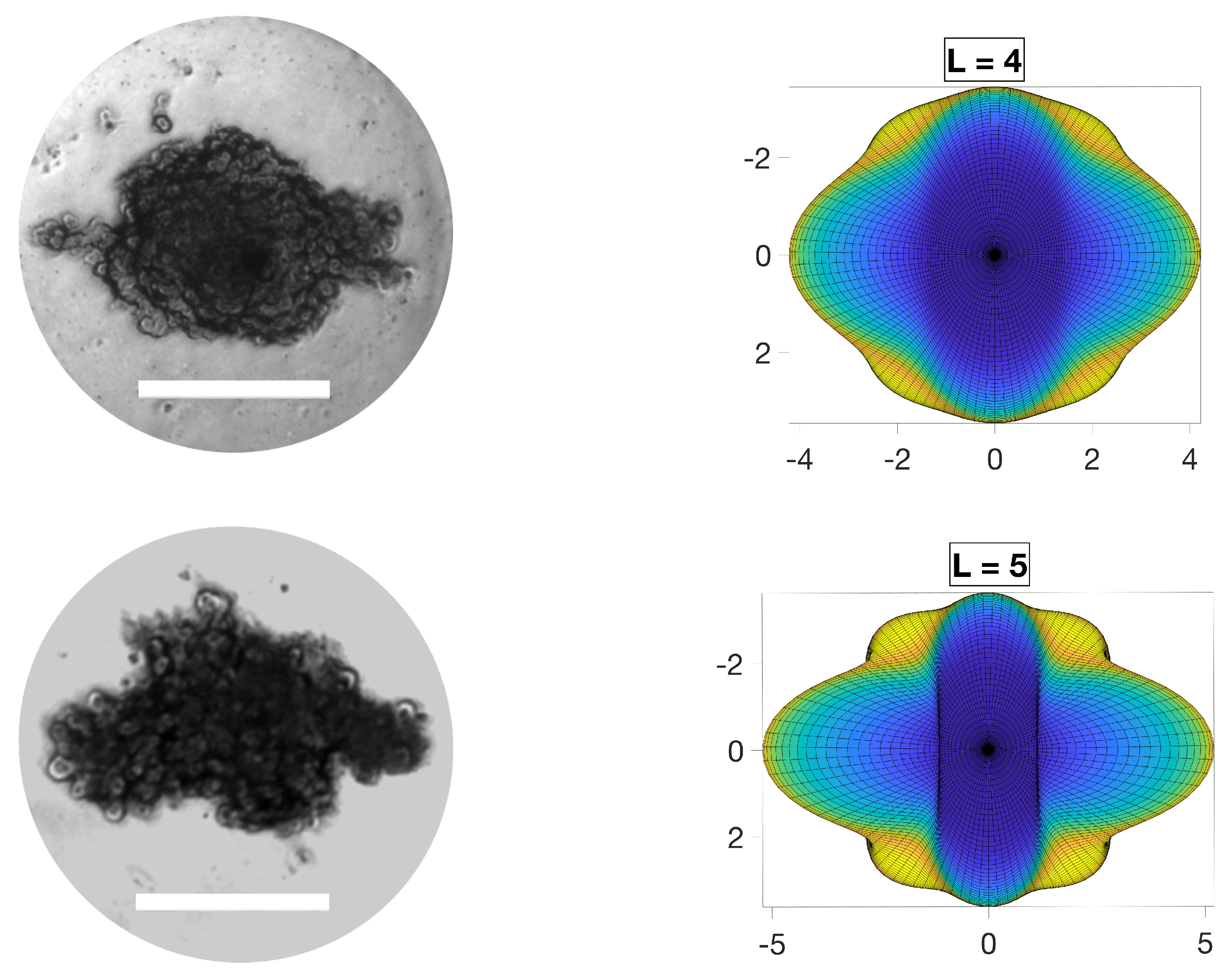
In this section, experimental results are compared to the model predictions presented in previous sections. To this end, the asymmetric modes were compared against the formation of in vitro solid tumor spheroids generated from a glioma cell line (U251 hGB cells). HGB cells were cultured in Dulbecco’s Modification of Eagle’s Medium (DMEM) supplemented with 10% (v/v) Fetal Bovine Serum (FBS) and 1% (v/v) Penicillin/Streptomycin and incubated at 37 °C in 5% CO₂. Cells were then dissociated with Gibco^TM Trypsin-EDTA (0.5%), centrifuged at 300× g (5 min) and counted using a Trypan blue assay. Self-filling micro-well arrays (SFMAs) were used to produce tumor spheroids [28]. Spheroids were then supplemented with fresh medium every 24 h to maintain the concentration of nutrients. To resemble the conditions considered in the analytical part as closely as possible, only approximately spherical tumor spheroids were selected, and only small spheriods of ∼200 μm diameter, to avoid heterogeneity in their cell population, such as hypoxic and necrotic cells. Presence of such heterogeneity violated the adopted assumption of linear nutrient consumption throughout the tumor, ${\eta }^{2}C$, $\eta =$ constant, as hypoxic cells normally switch their metabolism to anaerobic glycolysis where they consume glucose at a higher rate compared to normal cells. We also provided them with a constant concentration of nutrients $C_{\infty }$ at their boundary by regularly refreshing the medium. Although the spheroids were kept in a symmetric medium, asymmetric stimuli are always a part of the natural environment of tumors. Images of tumors were obtained using optical microscopy (Axio Observer, ZEISS, Oberkochen, Germany). Figure 5 shows images of a few representative examples of aspherical tumors frequently observed in experiments, compared with model predictions of the maximal asymmetric modes. The qualitative comparison showed that the tumor spheroids acquired configurations similar to the model predictions. It should be noted that the experimental results were limited in terms of quantitative measurements due to the complexity in implementation of the parameters of interest. For instance, the real system could only start from an approximately spherical shape. In addition, the environment could not be perfectly uniform. However, reasonable agreement was observed between the experimental results and the model predictions where the salient features of the tumor configurations aligned with the model predictions of configurations dominated by the growth of asymmetric modes.

5. Conclusions

The stability of the radially symmetric growth of tumor spheroids was studied by introducing asymmetric perturbations to the symmetric steady-state solution of a reaction-diffusion model in which the rate of nutrient consumption was concentration dependent. The analytical solution, expressed in terms of a spherical harmonic basis, manifested the growth of asymmetric modes. It was shown that the radially symmetric steady-state solution for the growth of tumor spheroids in a symmetric environment was unstable with respect to small asymmetric perturbations. Such perturbations excited asymmetric modes of growth. These modes could grow in time and dominate the tumor configuration. The number of such modes and their rates of growth depended on surface tension, external nutrient sources and the rate of nutrient consumption. A high nutrient source concentration allowed for a large tumor size, which increased the number of unstable excited asymmetric modes. However, high rates of nutrient consumption and surface tension led to a smaller size of the tumor and a smaller number of growing asymmetric modes. In addition, we showed that spherical tumors were unstable since asymmetric growing modes always dominated the tumor configuration. Hence, the spherical configurations of tumors, even under experimentally controlled symmetric conditions, were naturally unstable. These analytic results were in agreement with the configurations of growing in-vitro human glioblastoma (hGB) spheroids.

References

- Please, C.; Pettet, G.; McElwain, D. A new approach to modelling the formation of necrotic regions in tumours. Appl. Math. Lett. 1998, 11, 89–94. [Google Scholar] [CrossRef] [Green Version]
- Altrock, P.M.; Liu, L.L.; Michor, F. The mathematics of cancer: Integrating quantitative models. Nat. Rev. Cancer 2015, 15, 730–745. [Google Scholar] [CrossRef]
- Araujo, R.P.; McElwain, D.L.S. A history of the study of solid tumour growth: The contribution of mathematical modelling. Bull. Math. Biol. 2004, 66, 1039. [Google Scholar] [CrossRef]
- Landman, K.A.; Please, C.P. Tumour dynamics and necrosis: Surface tension and stability. Math. Med. Biol. J. IMA 2001, 18, 131–158. [Google Scholar] [CrossRef]
- Ward, J.P.; King, J.R. Mathematical modelling of avascular-tumour growth. Math. Med. Biol. J. IMA 1997, 14, 39–69. [Google Scholar] [CrossRef]
- Cristini, V.; Lowengrub, J. Multiscale Modeling of Cancer: An Integrated Experimental and Mathematical Modeling Approach; Cambridge University Press: Cambridge, UK, 2010. [Google Scholar]
- Chaplain, M.; Britton, N. On the concentration profile of a growth inhibitory factor in multicell spheroids. Math. Biosci. 1993, 115, 233–243. [Google Scholar] [CrossRef]
- Byrne, H.M.; Chaplain, M. Growth of necrotic tumors in the presence and absence of inhibitors. Math. Biosci. 1996, 135, 187–216. [Google Scholar] [CrossRef]
- Adam, J.A. A mathematical model of tumor growth. III. Comparison with experiment. Math. Biosci. 1987, 86, 213–227. [Google Scholar] [CrossRef]
- Casciari, J.; Sotirchos, S.; Sutherland, R. Mathematical modelling of microenvironment and growth in EMT6/Ro multicellular tumour spheroids. Cell Prolif. 1992, 25, 1–22. [Google Scholar] [CrossRef]
- Casciari, J.J.; Sotirchos, S.V.; Sutherland, R.M. Variations in tumor cell growth rates and metabolism with oxygen concentration, glucose concentration, and extracellular pH. J. Cell. Physiol. 1992, 151, 386–394. [Google Scholar] [CrossRef]
- Jiang, Y.; Pjesivac-Grbovic, J.; Cantrell, C.; Freyer, J.P. A multiscale model for avascular tumor growth. Biophys. J. 2005, 89, 3884–3894. [Google Scholar] [CrossRef] [PubMed] [Green Version]
- Amereh, M.; Edwards, R.; Akbari, M.; Nadler, B. In-Silico Modeling of Tumor Spheroid Formation and Growth. Micromachines 2021, 12, 749. [Google Scholar] [CrossRef] [PubMed]
- Hanahan, D.; Weinberg, R.A. Hallmarks of Cancer: The Next Generation. Cell 2011, 144, 646–674. [Google Scholar] [CrossRef] [Green Version]
- Bresch, D.; Colin, T.; Grenier, E.; Ribba, B.; Saut, O. Computational modeling of solid tumor growth: The avascular stage. SIAM J. Sci. Comput. 2010, 32, 2321–2344. [Google Scholar] [CrossRef]
- Yoo, Y.D.; Kwon, Y.T. Molecular mechanisms controlling asymmetric and symmetric self-renewal of cancer stem cells. J. Anal. Sci. Technol. 2015, 6, 18. [Google Scholar] [CrossRef] [PubMed] [Green Version]
- Benzekry, S.; Lamont, C.; Barbolosi, D.; Hlatky, L.; Hahnfeldt, P. Mathematical modeling of tumor–tumor distant interactions supports a systemic control of tumor growth. Cancer Res. 2017, 77, 5183–5193. [Google Scholar] [CrossRef] [Green Version]
- Mascheroni, P.; Carfagna, M.; Grillo, A.; Boso, D.; Schrefler, B.A. An avascular tumor growth model based on porous media mechanics and evolving natural states. Math. Mech. Solids 2018, 23, 686–712. [Google Scholar] [CrossRef]
- Byrne, H.; Chaplain, M. Modelling the role of cell-cell adhesion in the growth and development of carcinomas. Math. Comput. Model. 1996, 24, 1–17. [Google Scholar] [CrossRef]
- Li, C.K.N. The glucose distribution in 9l rat brain multicell tumor spheroids and its effect on cell necrosis. Cancer 1982, 50, 2066–2073. [Google Scholar] [CrossRef]
- Cui, S. Analysis of a mathematical model for the growth of tumors under the action of external inhibitors. J. Math. Biol. 2002, 44, 395–426. [Google Scholar] [CrossRef]
- Cui, S.; Friedman, A. Analysis of a mathematical model of the effect of inhibitors on the growth of tumors. Math. Biosci. 2000, 164, 103–137. [Google Scholar] [CrossRef] [Green Version]
- Li, X.; Cristini, V.; Nie, Q.; Lowengrub, J.S. Nonlinear three-dimensional simulation of solid tumor growth. Discret. Contin. Dyn. Syst. B 2007, 7, 581. [Google Scholar] [CrossRef]
- Cristini, V.; Lowengrub, J.; Nie, Q. Nonlinear simulation of tumor growth. J. Math. Biol. 2003, 46, 191–224. [Google Scholar] [CrossRef]
- Wu, J.; Cui, S. Asymptotic behaviour of solutions of a free boundary problem modelling the growth of tumours in the presence of inhibitors. Nonlinearity 2007, 20, 2389. [Google Scholar] [CrossRef]
- Langer, J.S. Instabilities and pattern formation in crystal growth. Rev. Mod. Phys. 1980, 52, 1. [Google Scholar] [CrossRef]
- Byrd, B.K.; Krishnaswamy, V.; Gui, J.; Rooney, T.; Zuurbier, R.; Rosenkranz, K.; Paulsen, K.; Barth, R.J. The shape of breast cancer. Breast Cancer Res. Treat. 2020, 183, 403–410. [Google Scholar] [CrossRef]
- Seyfoori, A.; Samiei, E.; Jalili, N.; Godau, B.; Rahmanian, M.; Farahmand, L.; Majidzadeh-A, K.; Akbari, M. Self-filling microwell arrays (SFMAs) for tumor spheroid formation. Lab Chip 2018, 18, 3516–3528. [Google Scholar] [CrossRef]
Figure 1.
Tumor growth rate, , vs. R for various values of nutrient supply in (a), nutrient consumption in (b) and surface tension in (c). A maximum of two plausible steady-state solutions existed, which could be stable () or unstable (). It could be seen that the maximum of two steady-state solutions was achieved for sufficient nutrient supply (a), low consumption rate (b) and low surface tension (c).
Figure 2.
Growth rate of asymmetric modes with respect to for four choices of mode number . In each sub-figure, the radii where the curves cross indicate the steady-state solutions, i.e., . In (a) and (b) ; the number of unstable asymmetric modes for was reduced by lowering the nutrient source . For instance, for , the steady state was unstable in (b), while reducing stabilized it in (a). In (c) and (d) ; a higher rate of consumption led to smaller steady-state with a smaller number of unstable asymmetric modes. In (e) and (f) ; reducing the surface tension allowed for larger steady-state , while more asymmetric modes became unstable. In all cases, was unstable to low-mode numbers, but was stable with respect to sufficiently large mode numbers.
Figure 3.
Growth rate of asymmetric modes with respect to l (mode number) for and . The mode number that maximized the asymmetric growth rate (maximal mode) is marked in red, indicating that increasing surface tension dropped the dominant mode from to for ; however, it had a fixed value of for .
Figure 4.
The asymmetric configuration of a tumor for two different choices of parameters, (a-1,a-2) , the corresponding growing modes , (b-1,b-2) and the corresponding unstable modes . The top (left) and side (right) views are shown in the figure. Colors represent the value of the z component of the radius; yellow means .
Figure 5.
Asymmetric configurations of in vitro human glioblastoma (hGB) spheroids (left column) compared with the similar configurations of maximal asymmetric modes predicted by the model (right column). Nearly spherical tumors with no heterogeneity in their cell population were provided with constant concentration of nutrients at their boundary to resemble a symmetric environmental condition. Scale bars are 200 μm.
Publisher’s Note: MDPI stays neutral with regard to jurisdictional claims in published maps and institutional affiliations. |
© 2022 by the authors. Licensee MDPI, Basel, Switzerland. This article is an open access article distributed under the terms and conditions of the Creative Commons Attribution (CC BY) license (https://creativecommons.org/licenses/by/4.0/).
Share and Cite
MDPI and ACS Style
Amereh, M.; Bahri, Y.; Edwards, R.; Akbari, M.; Nadler, B. Asymmetric Growth of Tumor Spheroids in a Symmetric Environment. Mathematics 2022, 10, 1955. https://doi.org/10.3390/math10121955
AMA Style
Amereh M, Bahri Y, Edwards R, Akbari M, Nadler B. Asymmetric Growth of Tumor Spheroids in a Symmetric Environment. Mathematics. 2022; 10(12):1955. https://doi.org/10.3390/math10121955
Chicago/Turabian StyleAmereh, Meitham, Yakine Bahri, Roderick Edwards, Mohsen Akbari, and Ben Nadler. 2022. "Asymmetric Growth of Tumor Spheroids in a Symmetric Environment" Mathematics 10, no. 12: 1955. https://doi.org/10.3390/math10121955
Note that from the first issue of 2016, this journal uses article numbers instead of page numbers. See further details here.