
A New Case-Mix Classification Method for Medical Insurance Payment


1
Key Laboratory for Applied Statistics of MOE, School of Mathematics and Statistics, Northeast Normal University, Changchun 130024, China
2
Faculty of Mathematics, Kim Il Sung University, Pyongyang 999093, Democratic People’s Republic of Korea
*
Authors to whom correspondence should be addressed.
Mathematics 2022, 10(10), 1640; https://doi.org/10.3390/math10101640
Submission received: 14 April 2022
/
Revised: 3 May 2022
/
Accepted: 7 May 2022
/
Published: 11 May 2022
(This article belongs to the Special Issue Statistical Modeling for Analyzing Data with Complex Structures)
Abstract
:Rapidly rising medical expenses can be controlled by a well-designed medical insurance payment system with the ability to ensure the stability and development of medical insurance funds. At present, China is in the stage of exploring the reform of the medical insurance payment system. One of the significant tasks is to establish an appropriate reimbursement model for disease treatment expenses, so as to meet the needs of patients for medical services. In this paper, we propose a case-mixed decision tree method that considers the homogeneity within the same case subgroup as well as the heterogeneity between different case subgroups. The optimal case mix is determined by maximizing the inter-group difference and minimizing the intra-group difference. In order to handle the instability of the tree-based method with a small amount of data, we propose a multi-model ensemble decision tree method. This method first extracts and merges the inherent rules of the data by the stacking-based ensemble learning method, then generates a new sample set by aggregating the original data with the additional samples obtained by applying these rules, and finally trains the case-mix decision tree with the augmented dataset. The proposed method ensures the interpretability of the grouping rules and the stability of the grouping at the same time. The experimental results on real-world data demonstrate that our case-mix method can provide reasonable medical insurance payment standards and the appropriate medical insurance compensation payment for different patient groups.
MSC:
62P10; 62H301. Introduction
In recent years, the rapid increase in health care costs has become a troublesome issue, and the diagnosis and treatment of diseases often face intrinsic complexity and uncertainty. Therefore, the reform and improvement of medical insurance payment methods have always been anticipated in the medical community. A good medical insurance payment system should not only control the expenditure of medical insurance funds and restrain unreasonable medical behaviors, but also fairly compensate medical costs and expenses to ensure the quality and enthusiasm of medical services. Reference [1] proposed a novel case-mix classification scheme, the diagnosis related groups system (DRGs), which comprehensively considers factors such as disease diagnosis, disease severity, and intensity of medical service usage, and establishes a suite of clinical case classification methods based on medical resource consumption. Due to the wide applicability to practical situations, this method has played a positive role in promoting the medical service system in the United States and effectively controlled the growth of medical expenses [2,3]. Therefore, many countries followed them to develop their own DRG grouping system [4,5]. However, the differences in healthcare ecosystems between countries cause the DRGs not to work equally well everywhere. In 2020, the Chinese National Healthcare Security Administration proposed the Big Data Diagnosis-Intervention Packet (DIP) grouping scheme. From a large amount of data, DIP extracts features that are closely related to the patient’s medical resource consumption level and combines cases through these features [6].
The case-mix model is essentially a disease grouping system designed to improve the quality of care or cost management. In general, research on medical expenses is based on various regression models to predict disease costs [7]. However, in case-mix studies, it is more important to classify patients into clinically meaningful and understandable groups that consume similar healthcare resources. Tree methods are often used to build case-mix models inspired by their advantages of intuitive and interpretable representations. Numerous authors have proposed different tree-based models. Reference [8] conducted a study on the diagnosis-related grouping of inpatient medical expenses in colorectal cancer patients based on a decision tree model. Reference [9] proposed a method to build the regression trees by bootstrap and use them for model retrieval in DGR systems. The authors in [10] generated diagnostically relevant groups through the CHAID model and provided a more accurate estimate of case-mix costs. Reference [11] investigated the diagnosis-related grouping of senile cataracts based on the E-CHAID algorithm. However, the tree-based models also have some drawbacks, with the undesirable tendency to overfit the data. Furthermore, tree structures are notoriously unstable, especially when the number of training samples is small, and small perturbations in the training set may cause large changes in the generated classes [12]. The diversity of tree structures also comes from different greedy search algorithms used to identify trees. In the related literature, there are generally two approaches used to deal with tree model instability: model selection and model combination. The advantage of choosing a single tree model is that simple and interpretable rules can be produced through faster computation. Similar approaches are based on selecting a single representative decision tree using a metric that evaluates the similarity or distance between trees, see [13,14]. However, these methods are mainly used in classification problems, and the accuracy and stability of such a single tree are not as good as those of an ensemble method. Ensemble learning usually achieves higher accuracy and better generalization ability than a single classifier by generating multiple models and combining them to obtain the final prediction result [15]. Common ensemble learning methods include packing, boosting, stacking, and Bayesian model averaging [16,17,18,19]. For some problems in the medical and bioinformatical community, it is more important to extract useful knowledge from the data rather than an accurate model. Therefore, the output of the learning model should be accurate, stable, understandable, and acceptable to people. However, most of the existing ensemble methods focus on improving the accuracy of prediction models, while ignoring the interpretability. In addition, feature selection is an important step in the process of constructing a reasonable case mix. Especially when the data dimension is relatively high, one can select the optimal input feature set from a given dataset, allowing machine learning models to better understand and distinguish the patterns in dataset more efficiently. At the same time, reducing the data dimension is beneficial to shorten the time for subsequent computation. In recent studies, several hybrid metaheuristic-based methods have been applied to solve the feature selection problem and achieved good results. For example, reference [20] proposed a genetic algorithm-based hierarchical feature selection (HFS) model to optimize local and global features extracted from images. Reference [21] proposed a binary hybrid metaheuristic-based algorithm and applied it to feature selection for COVID-19 classification.
Most of the traditional case-mix methods consider the variability among patients from a medical point of view. In contrast to these methods, this study focuses on the development of data-driven methods with the motivation to explore the differences in medical costs among different patients and to give intuitive case-mix rules. The main work and contributions of this paper are as follows: First, we propose a new case-mix decision tree model. We define a new objective function to evaluate the differences in medical resource consumption between different subgroups of cases. Minimizing this objective function leads to simultaneously maximizing the difference in medical resource consumption between heterogeneous groups and minimizing the difference within homogeneous groups. Second, considering that the tree method tends to become unstable as the amount of data is small, we borrow the idea of stacking to extract the internal rules of the data by multiple learners of different types and combine the models based on the least-squares method. At the same time, in order to avoid the overfitting problem, we shrink the coefficients using the norm as a penalty term. A new sample set is constructed using the original data and the generated rules, and a case-mix tree model is built from it. This method exploits more model information through integration and improves the accuracy and reliability of grouping results. Finally, we validate the effectiveness of the method on real-world data and formulate an appropriate case-mix payment standard.
The rest of the paper is organized as follows. In Section 2, we give a detailed introduction of the proposed case-mix decision tree model and multi-model ensemble decision tree method. In Section 3, the grouping performances of the proposed method in comparison with CART and CHAID are evaluated under various scenarios through simulation experiments. In Section 4, from the case data provided by the Jilin Province Administration of Social Medical Insurance of China, we construct an ovarian cancer case-mix model and formulate a payment standard to provide the reference for the medical expense reimbursement of ovarian cancer patients. Finally, we conclude the paper in Section 5.
2. Methodology
This paper proposes a multi-model ensemble decision tree model to solve the problem of case-mix and group payment, and generates an interpretable model while ensuring reasonable grouping. In the first subsection, we introduce the case-mix decision tree model (CDT). The second part describes the multi-model ensemble decision tree method (MEDT).
2.1. Case-Mix Decision Tree
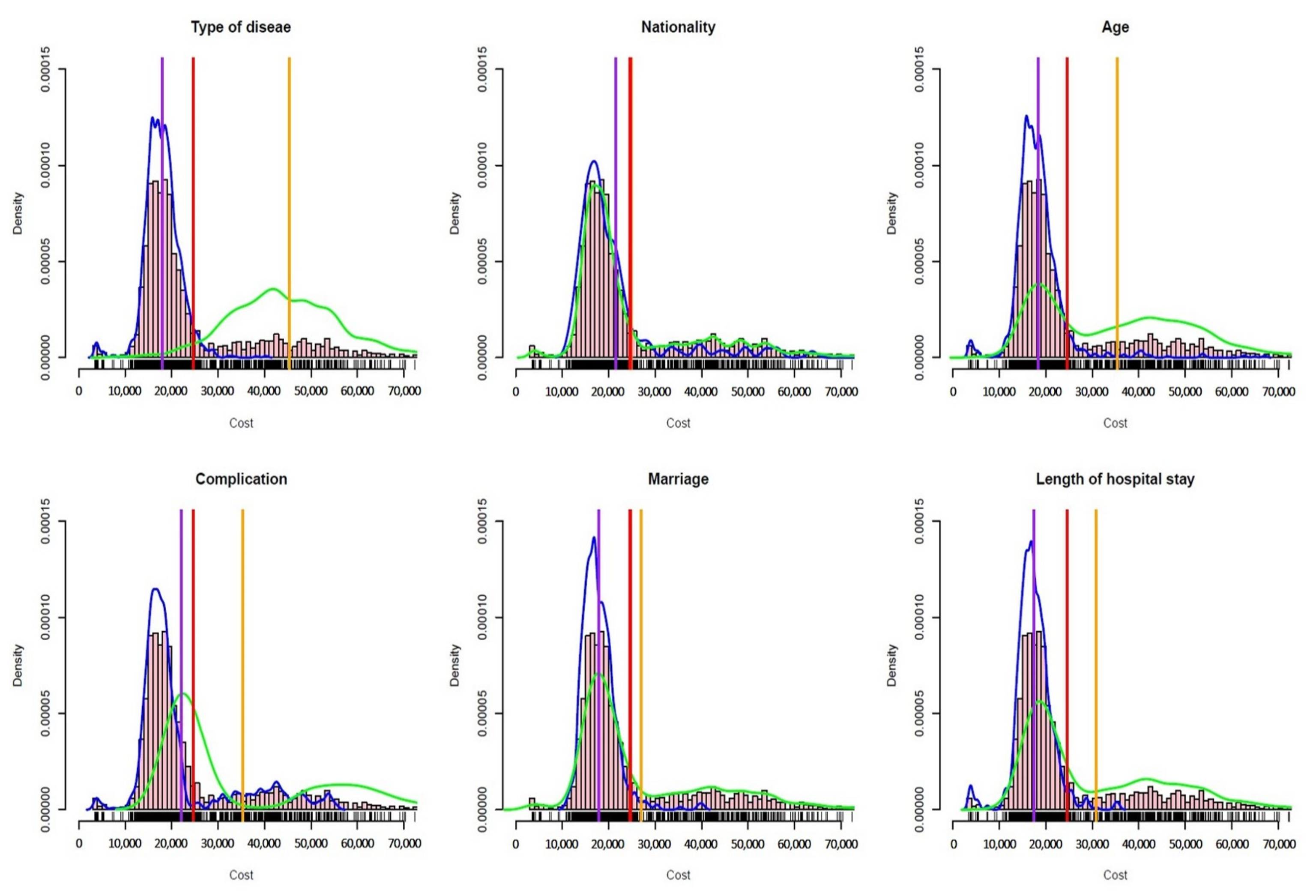
Traditional decision trees are generally used to solve classification and regression problems. They recursively divide the data space by optimizing a specific objective function and generate multiple disjoint partitions [22]. The sub-nodes corresponding to each partition have different partitioning characteristics. Therefore, we can regard each partition as a different cluster. The objective functions used to select and divide features generally vary according to different problems. For example, the information gain ratio is used in the classical C4.5 algorithm, and the Gini index or squared error is used in CART. In the case-mix problem, we intend to merge different cases into groups, formulate the medical payment standard for different case mixes according to the medical resources they consume, and recommend reasonable medical insurance compensation payments for them [23]. The case-mix methods mainly depend on the selection of grouping features, which leads to different grouping outputs. For example, in the case-mix of patients with cerebral infarction, different clusters will be formed using different grouping features, as shown in Figure 1. In Figure 1, the blue and green lines represent the density of the cost distribution for two different patient groups, the purple and orange lines represent the average cost of the two different disease groups, and the red line represents the cost of all patients’ mean. From Figure 1, we can see that different grouping characteristics have significant differences in the degree of differentiating the patient. When the disease type is selected as the grouping characteristic, the degree of differentiating patients between the two disease groups is more obvious, and the difference between different groups is large. When choosing ethnicity or marital status as the dividing feature, the difference between the two groups is hardly distinguishable.
We aim to find a reasonable grouping method, which satisfies the following two properties: first, the difference between the groups should be large enough to indicate that different groups have significant differences in the consumption of medical resources, so as to identify the needs of different patients for medical care; second, the differences between groups should be as small as possible, indicating that patients in the same group have similar medical needs. From these perspectives, we propose a new method for selecting features via a decision tree.
Let X and Y denote the explanatory variable and the target variable, respectively, D to be the dataset , and be M sub-regions divided into the feature space. Here, j and s represent the segmentation variable and segmentation point, respectively. If we select the j-th variable at first and use s as a split point, two sub-regions can be defined as follows:
To represent the in-group difference, we adopt the following in-group variance:
where represents the consumption level of the i-th patient’s medical resources, which can be reflected in medical expenses, and represent the mean value of medical expenses in the sub-region and , respectively. The smaller the intra-group variance, the smaller the difference in intra-group medical resource consumption between the two disease groups after segmentation, providing stronger homogeneity.
To measure the difference of medical resource consumptions between different disease groups, the mean squared distance between groups is used as follows:
where is the mean value of the medical expenses of all cases before grouping the current sample set. The larger the mean squared distance between groups, the greater the difference between the two disease groups after grouping, providing the stronger heterogeneity between groups.
It is necessary to measure the efficiency of different grouping methods, so we define a grouping objective function:
For a case-mix method, it is better to make the differences between groups as large as possible, and the differences within groups as small as possible. Finding the best grouping method can be turned into an optimization problem . The solution to this problem is similar to regression trees. The greedy algorithm can be used to traverse all split variables j, and for the fixed split variable j, traverse all of the split points s, so as to find the optimal splitting. The split variable and split point form a pair of . The input space is divided into two regions in turn, and the above division process is repeated on each region until the stop condition is satisfied. The CDT algorithm is as follows:
Step 1: Find the optimal segmentation variable j and the segmentation point s by solving
Traverse every segmentation variable j and the corresponding segmentation point s, and select the pair that minimizes the objective in Equation (5).
Step 2: Use the selected pair to divide the area and determine the corresponding output.
Step 3: Continue to repeat Steps 1 and 2 for the two sub-regions until the stop condition is satisfied.
Step 4: Divide the input space into M sub-regions , for a sample x, the value is given by
where is the indicator function, and all pairs correspond to the splitting characteristics of .
A “fully grown” tree often overfits the data, so it is necessary to set a certain early-stop condition during the tree’s growth. Furthermore, a procedure analogous to backward selection is used to prune the tree by cutting off the unneeded leaf nodes [24]. A tree T with leaf nodes is defined as
Then, we calculate the cost-complexity [25] for tree T with the following formula:
where is the cost-complexity parameter, and is the number of leaf nodes in the tree. For a fixed , there exists a subtree that minimizes , denoted by . Note that the optimal subtree tends to be simple for large and complex for small . Reference [25] showed that the tree sequence minimizing is nested and trees can be pruned recursively, in which cross-validation is commonly used to choose an appropriate subtree.
2.2. The MEDT Algorithms
Due to the data collection burden and personal privacy issues, the amount of case data is often relatively small, making the single-tree model prone to structural instability. To address this issue, this paper proposes and evaluates a novel model combination method that combines the predominant accuracy and stability of multiple models with the interpretability of a single model. This method utilizes a stacking method to combine the metadata generated by multiple base learners through a meta-learner. We can regard that during the model combination, the multiple learners jointly learn from the data, extract rules, and then combine the rules in some way to produce a new model. This model is based on the understanding of the data generated by multiple learners—a mapping of multiple models in general, consequently leading the differentiating of their rules to become complicated. Many factors, such as the patient’s physiological characteristics, disease degree, and treatment received, are closely related to the medical resources consumed by the patient. In the case-mix problem, we intend to find features that have significant impacts on patient healthcare costs and divide the population into different subgroups based on these features. In this way, the reference of medical expenses under different subgroups can be obtained. A good grouping method can show the degree of influence of different features on the results, while demonstrating the obtained rules in an intuitive and understandable way, such as a hierarchical structure or a tree diagram. The model obtained by the combination of meta-learners can be considered as an explanation of the patient’s physiological characteristics, disease degree, received treatment, and medical resources consumed. Although this explanation may not be clear enough, it does not impact the grouping of patients generated according to the importance of features. On the premise that the learned model is “true”, we can extract a variety of rules through the above method and combine them to give an “explanation” of the data generation mechanism. To avoid overfitting problems, we use K-fold cross-validation and build a new set of synthetic samples based on this newly generated “rule”, which is aggregated with the original training set to form a new test set. This new test set contains not only the information in the original data but also the “rule” information extracted by various learners, leading the information contained to be more comprehensive. In general, the accuracy and stability of the learner tend to improve with the size of the training set. Therefore, more accurate and stable case-mix pricing results can be obtained based on the new test set than based on the original data. The procedure just described will be called multi-model ensemble decision tree (MEDT), as shown in Algorithm 1.
| Algorithm 1 The MEDT algorithm. |
|
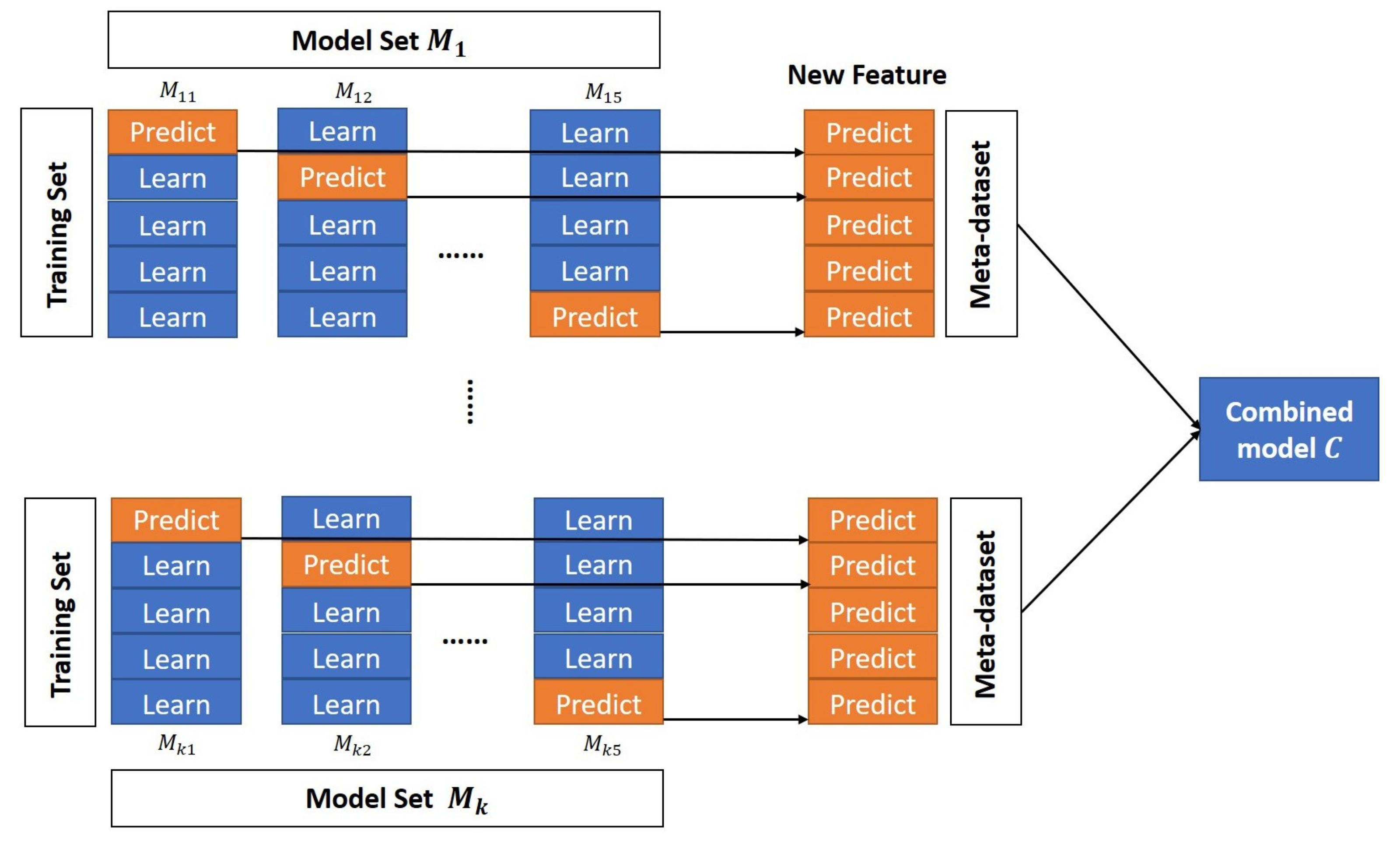
During the actual case-mix process, we usually select the base learner from a variety of strong learners, such as random forest, gradient boosting decision tree (GBDT), extreme gradient boosting (XGBoost), lasso regression, support vector regression (SVR), and other models. The advantage of this setting is that the proposed ensemble model takes the prediction capability for linear and nonlinear structures into account, and that the selected models have strong abilities to distinguish the variable importance, which can identify the most important variables that affect the degree of medical resource consumption. While ensuring the generalization ability of the model, we intend to preserve the information of the original data as much as possible. We adopt the five-fold cross-validation method, so we randomly divide the original data into five parts, out of which four parts are used as a training set and the remaining one is used as a validation set. The base learner is trained using the training data and the predictions produced by the base learner are used as metadata. Metadata can be regarded as the input features of the metamodel. Next, we will use the metadata to train the metamodel (the combined model C). Figure 2 shows the above learning process.
Model combination has great significance in the procedure of ensemble construction. The appropriate combination can improve the data analysis ability of the model. The most common combination method is majority voting and its variants [26], such as simple majority voting and weighted majority voting. In this paper, we investigate the stacking-like approach to constructing the ensemble, so as to explore a better way to combine trained base learners. Each base learner provides a different contribution to the final results, which can be represented as a weight. In this case, the question is turned into how to predefine the weights. Reference [26] proposed a stacked regression method. This method improves the prediction accuracy by linearly combining the different predictors, and determines the weight of each predictor by the least-squares method. Since we choose the base learners among strong ones, there is a strong correlation between the prediction results of the models. Using the least-squares method to assign weights to the model often causes overfitting. Here, we use the ridge regression method to determine the weights of the model:
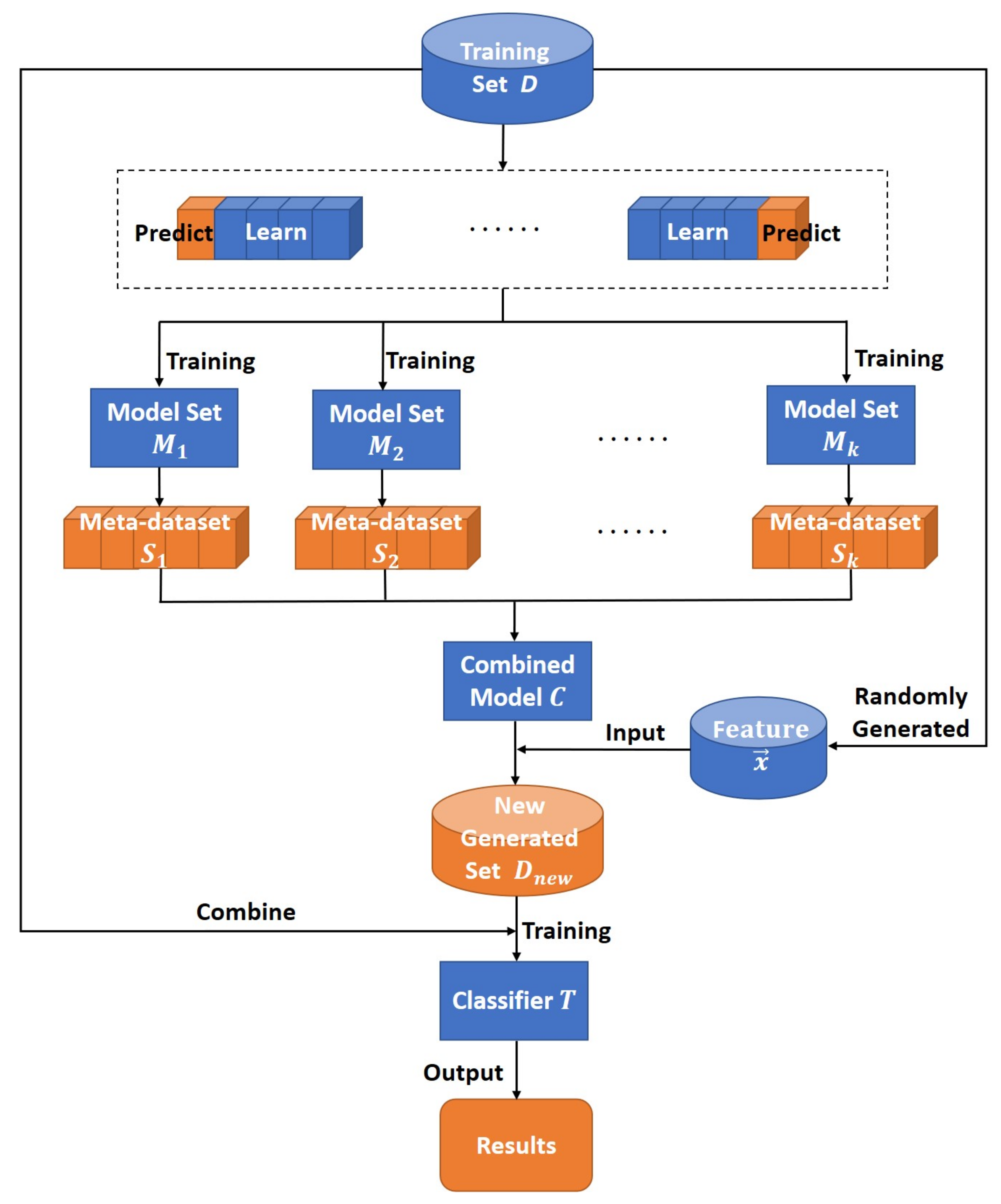
where is the penalty item, denotes the predictions of k different models, and is the weight of the i-th model. When combining the models, we shrink the weights of the models by adding the norm. This can tackle the overfitting problem, improve the generalization ability of the model, and better integrate multiple models to analyze the data. Then, we obtain the additional samples by applying the rules obtained with the ensemble model, then generate a new sample set D by aggregating those with the original data, and finally use D to construct a case-mix decision tree. Figure 3 shows the specific process of the MEDT algorithm.
3. Simulation Study
We compare the performance of multi-model ensemble decision tree methods in terms of several criteria over some simulation scenarios. We generate an outcome y through a certain model with four categorical covariates ( Multinomial (0.35, 0.4, 0.25), Bernoulli (0.7), Bernoulli (0.45), and Multinomial (0.15, 0.2, 0.4, 0.25)) and two continuous covariates ( (14, 25), (0, 1)).
Several parameters are inspected to assess the prediction performance under various simulation scenarios. First, we change the sample size n. Next, we invoke three types of data generation schemes, where , and are unrelated variables to y, and the error . In the first case, the outcome y is obtained by a linear model. In the second case, the outcome y is generated in a way that includes a polynomial term, a logarithmic term, and interaction terms. The third case is more complicated than the second one, with the participation of an exponential term.
Caes 1:
Case 2:
Case 3:
For each of the above scenarios, we augmented with additional 1000 samples generated by simulation. We split each dataset into the training and testing sets, one of which was randomly assigned half of that dataset and the other as its complement. Since class labels are not provided in our data, we evaluated the performance of the aforementioned methods based on cluster internal information [27]. We calculated the Calinski–Harabaz index (CHI), silhouette coefficient (SC), and Davies–Bouldin index (DBI) based on the testing set.
We conducted two simulation experiments. In the first experiment, we considered the settings with sample sizes n of 1000, 2000, and 4000, in which the training set and the test set each accounted for 50% of the dataset. We compared the performance of CART and CHAID with the proposed MEDT. The larger the values of CHI and SC, the smaller the value of DBI, indicating that the generated clusters are dense within the same cluster and that the different clusters are farther apart, i.e., the results of the case-mix are more significant.
It can be seen from Table 1 that when the sample size was relatively small (n = 1000), our proposed MEDT method exploited more sample information, so its performance was significantly better than the other two methods, with larger CHI and SC values and a smaller DBI value. Additionally, CART and CHAID may have under-fitting problems when the sample size is small, leading to inaccurate final grouping results. In addition, as the sample size increased, the performance of the three methods improved their results in terms of all metrics. When the sample size was increased from n = 1000 to n = 2000, the performance of CART and CHAID was significantly improved, but the clustering effect was still worse than our method. When the sample size became larger (n = 4000), the differences between the above three methods were subtle, but MEDT and CART performed relatively well. The results of the first simulation experiment show that the MEDT method performs better in the case of small samples. This is due to the fact that the MEDT method obtains more sample information by integrating more models.
Next, we verified that this approach favors better clustering (especially when the sample size is relatively small). In the second experiment, we had two different settings: in the first setting, we duplicated samples of the original training set and aggregated them into a new test set to train our proposed case-mix tree model, denoted as COM hereafter; in the second setting, we used the MEDT method directly on the training set data. As in the first simulation, we set the sample size n to be 600 and 1000 and generated the data. The training set and the test set each accounted for 50%, and Table 2 shows the comparative performance under two different settings.
The results in Table 2 show that when the sample size was small, the MEDT method could obtain better clustering results by utilizing more sample and model information. At the same time, we can see that applying the MEDT led to a slight increase in MSE compared with the method of directly duplicating samples, but this increase is hardly distinguishable. For the case-mix problem, we are more interested in the clustering of homogeneous patients than the accuracy of individual prediction. A reasonable grouping of cases will help health insurance departments to differentiate patients and make compensatory payments. In terms of the three metrics CHI, SC, and DBI, the MEDT method has better performance than that of direct sample duplication.
In some clinical scenarios, we often need to group patients in order to homogenize similar populations. However, when the amount of available data is insufficient, methods such as CART and CHAID do not perform so well, and the improvement brought about by simply copying the sample is also limited. In this case, the MEDT method performs better in grouping problems than the two comparative methods while keeping the predominant interpretability of the decision tree method. In the following section, we construct the case-mix of ovarian cancer patients based on this MEDT method.
4. Application
We conducted the experiment using the data of ovarian cancer (OC) patients in some tertiary hospitals in Jilin Province, China. This dataset was provided by the Jilin Province Administration of Social Medical Insurance of China and contains medical consumption records of OC patients from 2017 to 2019, patients’ individual information (including age, gender, marital status, ethnicity, medical insurance category, etc.), medical diagnosis information (including disease name, main medical operations, comorbidities, complications, etc.), and medical expenses (total amount of consumption and various medical service expenses). The features in the original data are not presented as a formalized vector but disorderly displayed as multiple records. Therefore, in order to conduct our subsequent experiments, we first preprocessed the data and quantified the categorical variables.
4.1. Ovarian Cancer Case-Mix Pricing
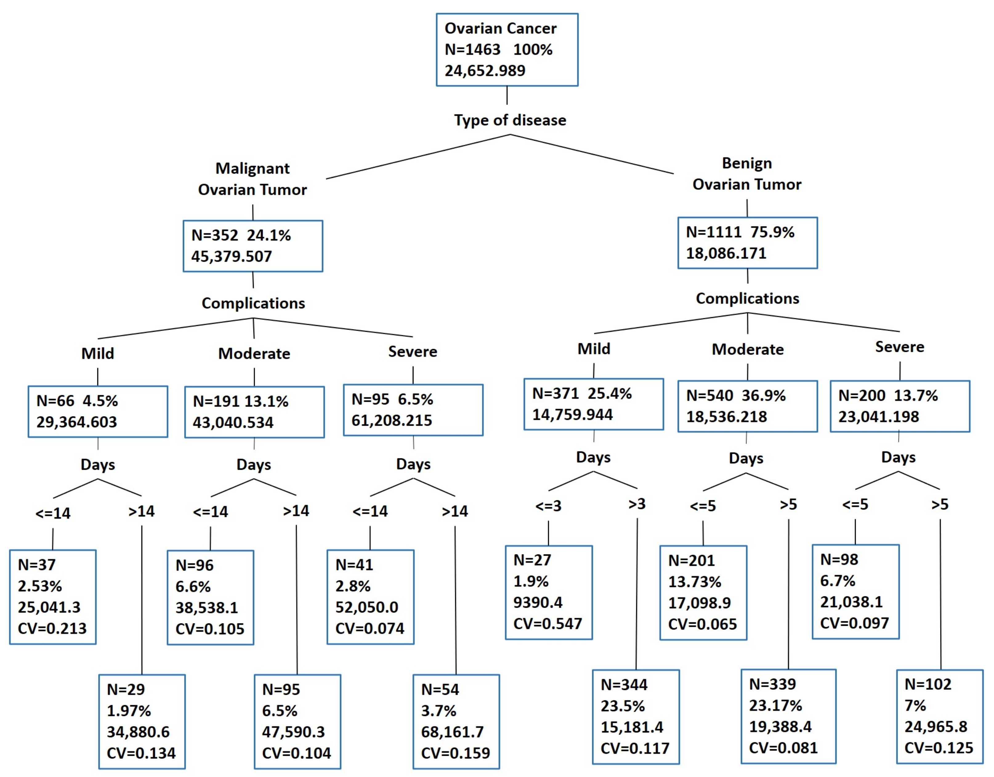
After preprocessing, we had 1463 OC cases. Next, we needed to price the case-mix according to the difference in medical resource consumption of patients. First, we used the MEDT method to build the case-mix model. The depth of the tree is proportional to the complexity of the model. Therefore, we set the maximum depth of the tree to 4 and pruned it. Figure 4 shows that 12 different case subgroups were obtained using the MEDT method, and the final grouping results are very clear and interpretable.
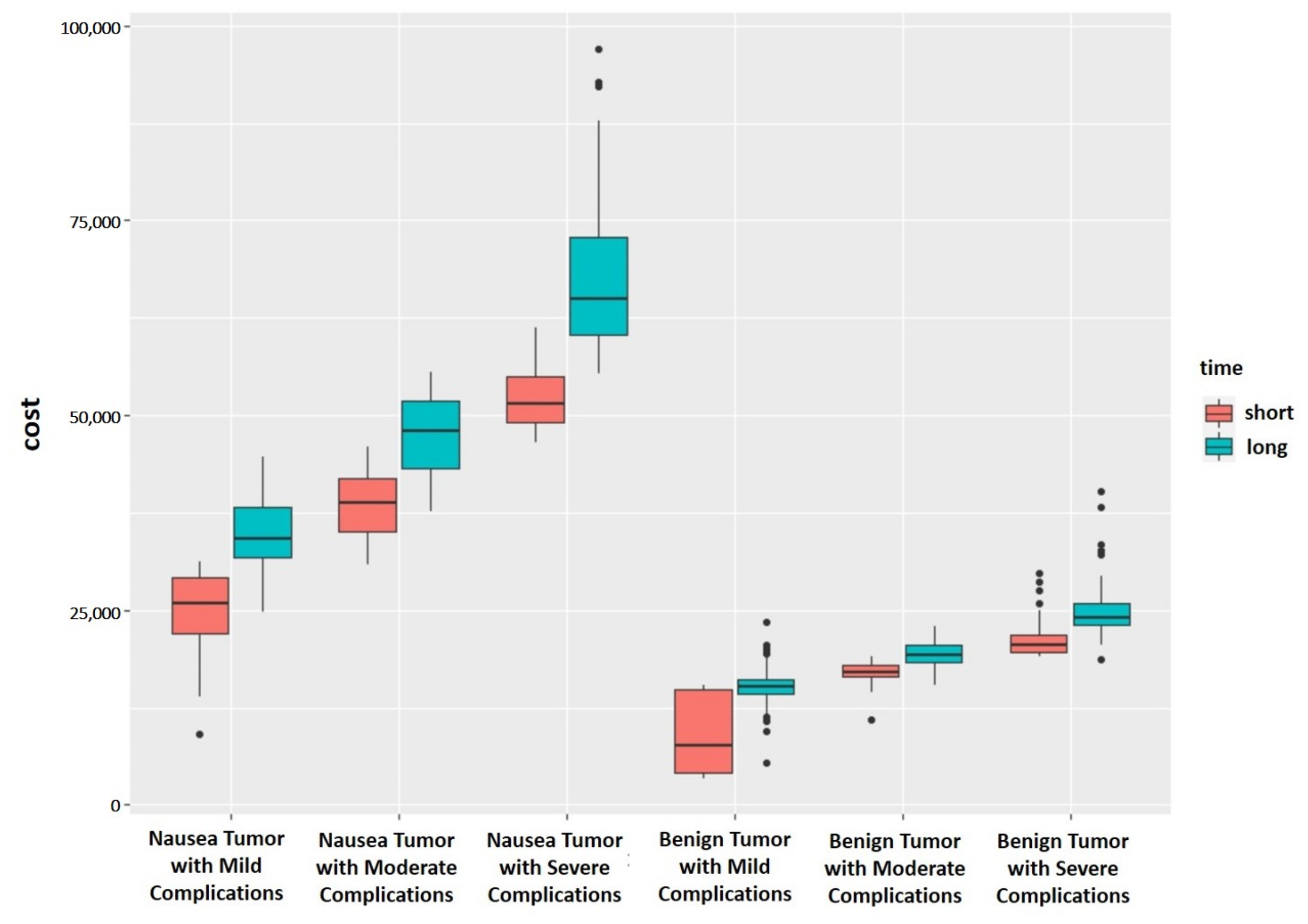
Then, we verified that our grouping is reasonable. Figure 5 shows the differences in medical expenses of 12 different OC case subgroups based on the MEDT method. As can be seen from Figure 5, the OC case subgroups obtained using our method are relatively separated, and each subgroup has different medical resource requirements. Afterward, we illustrated the rationality of grouping from the perspective of statistical tests. Firstly, we performed the Kruskal–Wallis test on the medical costs of patients in the 12 case subgroups, and obtained the p-value of the test is less than . Then, we performed multiple comparisons of case subgroups by Holm’s method [28]. Among them, the largest p-value in multiple comparisons was , which is still less than , indicating that there are significant statistical differences in the medical costs of patients between different case subgroups. These results from the statistical test verify that the proposed grouping method is reasonable.
Finally, we set a price for the ovarian cancer case-mix based on the grouping results in Figure 4 and compared it with the current payment standard for OC disease. In order to ensure consistency with the grouping criteria, we made small adjustments to the results of the case-mix. This helps the grouping criteria to be simple and comprehensible. Currently, the average reimbursement rate of medical insurance for treating OC is 70%. Therefore, we took 70% of the actual medical expenses of each case subgroup and rounded it to multiples of 500 to set as the corresponding payment standard for the OC case-mix. The results are shown in Table 3.
From Table 3, we can see that the payment standard for OC patients based on the MEDT method is more reasonable and interpretative. By grouping patients by differences in medical resource requirements, it cannot only meet the medical needs of mild patients but also increase the degree of medical compensation for severe patients, making the allocation of medical insurance funds more reasonable. At the same time, after applying the payment standard for the case mix, the total medical expenses of OC patients can be decreased by 9.12% compared with the previous standard. The standards developed by our method are also beneficial for controlling and reducing health care costs.
4.2. Result Comparison
We applied CART, CAHID, and our proposed MEDT method to build a case-mix tree model, and evaluated the performance of our method and comparative methods in terms of CV and RIV. The CV reflects the difference in medical resource consumption within each case subgroup, while the RIV reflects the degree of variance reduction after the case mix. A tree with a smaller CV value has a smaller degree of dispersion and better homogeneity, as well as smaller differences within the group. Similarly, a tree with a larger RIV can discover the better underlying rules in the data, provide more reasonable grouping, and reduce variations more [29]. According to the current technical specifications for DGR and DIP group payment by the National Medical Security Administration, the CV value after applying the case-mix should be less than 0.8, and the RIV value should be greater than 80%.
in which represents the average cost of the i-th case subgroup, represents the average medical cost of all patients, and represents the medical cost of the j-th patient in the i-th subgroup.
We set the same maximum tree depth and minimum sample number of leaf nodes for all three methods, and pruned the results of CART and MEDT. Then, we calculated the average CV and RIV values of the OC case-mix generated by the three methods. The results in Table 4 show that the grouping performance of the MEDT is better than the CART and CHAID methods, with a lower average CV value and a higher RIV value. Considering Table 3 together with Table 4, we can see that the CV values in the groups are all less than 0.8, indicating that the internal dispersion of each subgroup gets smaller after grouping. The RIV is 93.90%, which is greater than 0.8, indicating that the grouping method can discover more latent rules within the data, and the degree of systematization is higher. The grouping reduces the degree of variation by 93.90%, meaning that grouping has the capability to significantly reduce the degree of variation within the group.
In a nutshell, the simulation experiments’ results show that the proposed method outperforms the two comparative methods (CART, CHAID) in terms of reasonable metrics while better reflecting the heterogeneity between different case subgroups. Meanwhile, the results of experiments on real-world data show that the grouping by our method produces better CV and RIV values compared to the two other methods, which indicates that our method can perform better in the real dataset.
5. Conclusions
Faced with the rapid increase in medical expenses, the reform of medical insurance payments has become an imperative topic. At present, the medical insurance payments in China are mainly based on case-mix payment methods such as DRG and DIP. The good case-mix payment methods should generate reasonable groups and provide appropriate compensatory payments for patients with different medical resource needs. In this paper, we propose a case-mix decision tree method, which provides the reasonable grouping of patients with different medical resource needs as well as the predominant interpretability of tree models. In practical situations, provided data are often insufficient, causing the single-tree model to be structurally unstable. To handle this problem, we propose a multi-model ensemble decision tree method. During the model combination, we penalize by the ridge regression method to avoid the overfitting problem. Eventually, we construct a case-mix decision tree model and provide the interpretable grouping rules. The subgrouping experiments on both simulated and real-world data showed that our proposed method outperforms the two comparative methods (CART, CHAID).
The disadvantage of this method is that it requires more training time than a single decision tree, due to the integration of multiple models, especially when dealing with high-dimensional data. Furthermore, we have only conducted experiments on data with a few diseases. In the future, we can augment our dataset by collecting more cases from different medical centers to generate more reliable health insurance pricing models.
Author Contributions
Conceptualization, H.L., J.T. and W.Z.; Methodology, H.L., J.T. and W.Z.; Software, J.T. and K.J.; Validation, H.L. and K.J.; Resources, H.L.; Writing—original draft preparation, H.L., J.T. and K.J.; Writing—review and editing, W.Z. All authors have read and agreed to the published version of the manuscript.
Funding
This research is partially supported by the National Natural Science Foundation of China (Grant No. 12171077, 11771072), the National Key R&D Program of China (No. 2020YFA0714102), and the Science and Technology Development Plan of Jilin Province (20191008004TC).
Institutional Review Board Statement
Not applicable.
Informed Consent Statement
Not applicable.
Data Availability Statement
Not applicable.
Conflicts of Interest
The authors declare no conflict of interest.
References
- Fetter, R.B. Diagnosis related groups: Understanding hospital performance. Interfaces 1991, 21, 6–26. [Google Scholar] [CrossRef]
- Tatchell, M. Measuring hospital output: A review of the service mix and case mix approaches. Soc. Sci. Med. 1983, 17, 871–883. [Google Scholar] [CrossRef]
- Zindel, S.; Stock, S.; Müller, D.; Stollenwerk, B. A multi-perspective cost-effectiveness analysis comparing rivaroxaban with enoxaparin sodium for thromboprophylaxis after total hip and knee replacement in the German healthcare setting. BMC Health Serv. Res. 2012, 12, 1–14. [Google Scholar] [CrossRef] [PubMed]
- Pilla, J.; Hindle, D. Adapting DRGs: The British, Canadian and Australian experiences. Health Inf. Manag. 1994, 24, 87–93. [Google Scholar] [CrossRef]
- Duff, J. Financing to foster community health care: A comparative analysis of Singapore, Europe, North America and Australia. Curr. Sociol. 2001, 49, 135–154. [Google Scholar] [CrossRef]
- Qian, M.; Zhang, X.; Chen, Y.; Xu, S.; Ying, X. The pilot of a new patient classification-based payment system in China: The impact on costs, length of stay and quality. Soc. Sci. Med. 2021, 289, 114415. [Google Scholar] [CrossRef]
- Thorpe, K.E. The use of regression analysis to determine hospital payment: The case of Medicare’s indirect teaching adjustment. Inquiry 1988, 25, 219–231. [Google Scholar]
- Wu, S.W.; Pan, Q.; Chen, T. Research on diagnosis-related group grouping of inpatient medical expenditure in colorectal cancer patients based on a decision tree model. World J. Clin. Cases 2020, 8, 2484. [Google Scholar] [CrossRef]
- Grubinger, T.; Kobel, C.; Pfeiffer, K.P. Regression tree construction by bootstrap: Model search for DRG-systems applied to Austrian health-data. BMC Med. Inform. Decis. Mak. 2010, 10, 1–11. [Google Scholar] [CrossRef] [Green Version]
- Zeng, Y.; He, A.J.; Lin, P.; Sun, Z.; Fang, Y. Developing case-mix standards with the Diagnosis-related Groups for payment reforms and hospital management in China: A case study in Xiamen city. Int. J. Healthc. 2016, 2, 102–110. [Google Scholar] [CrossRef]
- Luo, A.J.; Chang, W.F.; Xin, Z.R.; Ling, H.; Li, J.J.; Dai, P.P.; Deng, X.T.; Zhang, L.; Li, S.G. Diagnosis related group grouping study of senile cataract patients based on E-CHAID algorithm. Int. J. Ophthalmol. 2018, 11, 308. [Google Scholar] [PubMed]
- Domingos, P. Knowledge discovery via multiple models. Intell. Data Anal. 1998, 2, 187–202. [Google Scholar] [CrossRef]
- Miglio, R.; Soffritti, G. The comparison between classification trees through proximity measures. Comput. Stat. Data Anal. 2004, 45, 577–593. [Google Scholar] [CrossRef]
- Weinberg, A.I.; Last, M. Selecting a representative decision tree from an ensemble of decision-tree models for fast big data classification. J. Big Data 2019, 6, 1–17. [Google Scholar] [CrossRef]
- Wang, Y.; Wang, D.; Geng, N.; Wang, Y.; Yin, Y.; Jin, Y. Stacking-based ensemble learning of decision trees for interpretable prostate cancer detection. Appl. Soft Comput. 2019, 77, 188–204. [Google Scholar] [CrossRef]
- Breiman, L. Bagging predictors. Mach. Learn. 1996, 24, 123–140. [Google Scholar] [CrossRef] [Green Version]
- Freund, Y.; Schapire, R.E. Experiments with a New Boosting Algorithm. In Proceedings of the Thirteenth International Conference on International Conference on Machine Learning, ICML’96, Bari, Italy, 3–6 July 1996; Morgan Kaufmann Publishers Inc.: San Francisco, CA, USA, 1996; pp. 148–156. [Google Scholar]
- Wolpert, D.H. Stacked generalization. Neural Netw. 1992, 5, 241–259. [Google Scholar] [CrossRef]
- Buntine, W.L. A Theory of Learning Classification Rules. Ph.D. Thesis, University of Technology Sydney, Sydney, Australia, 1990. [Google Scholar]
- Malakar, S.; Ghosh, M.; Bhowmik, S.; Sarkar, R.; Nasipuri, M. A GA based hierarchical feature selection approach for handwritten word recognition. Neural Comput. Appl. 2020, 32, 2533–2552. [Google Scholar] [CrossRef]
- Bezdan, T.; Zivkovic, M.; Bacanin, N.; Chhabra, A.; Suresh, M. Feature Selection by Hybrid Brain Storm Optimization Algorithm for COVID-19 Classification. J. Comput. Biol. 2022. [Google Scholar] [CrossRef]
- Loh, W.Y. Classification and regression trees. Wiley Interdiscip. Rev. Data Min. Knowl. Discov. 2011, 1, 14–23. [Google Scholar] [CrossRef]
- Horn, S.D.; Bulkley, G.; Sharkey, P.D.; Chambers, A.F.; Horn, R.A.; Schramm, C.J. Interhospital differences in severity of illness: Problems for prospective payment based on diagnosis-related groups (DRGs). N. Engl. J. Med. 1985, 313, 20–24. [Google Scholar] [CrossRef]
- Larsen, D.R.; Speckman, P.L. Multivariate regression trees for analysis of abundance data. Biometrics 2004, 60, 543–549. [Google Scholar] [CrossRef] [PubMed]
- Breiman, L.; Friedman, J.H.; Olshen, R.A.; Stone, C.J. Classification and Regression Trees; Routledge: London, UK, 2017. [Google Scholar]
- Breiman, L. Stacked regressions. Mach. Learn. 1996, 24, 49–64. [Google Scholar] [CrossRef] [Green Version]
- Liu, Y.; Li, Z.; Xiong, H.; Gao, X.; Wu, J. Understanding of Internal Clustering Validation Measures. In Proceedings of the 2010 IEEE International Conference on Data Mining, ICDM ‘10, Sydney, Australia, 13–17 December 2010; IEEE Computer Society: Washington, DC, USA, 2010; pp. 911–916. [Google Scholar]
- Derrac, J.; García, S.; Molina, D.; Herrera, F. A practical tutorial on the use of nonparametric statistical tests as a methodology for comparing evolutionary and swarm intelligence algorithms. Swarm Evol. Comput. 2011, 1, 3–18. [Google Scholar] [CrossRef]
- Palmer, G.; Reid, B. Evaluation of the performance of diagnosis-related groups and similar casemix systems: Methodological issues. Health Serv. Manag. Res. 2001, 14, 71–81. [Google Scholar] [CrossRef]
Figure 1.
Grouping based on different features. The blue and green curves represent the density of the distribution of different case subgroups, and the purple and orange lines represent the average cost of the corresponding subgroups. The red line represents the average cost before grouping.
Figure 1.
Grouping based on different features. The blue and green curves represent the density of the distribution of different case subgroups, and the purple and orange lines represent the average cost of the corresponding subgroups. The red line represents the average cost before grouping.

Figure 2.
Multi-model combination process.

Figure 3.
The overall procedure of the MEDT algorithm.

Figure 4.
Ovarian cancer case-mix based on the MEDT method.

Figure 5.
Differences in medical expenses among different groups.


Table 1.
Comparison of CART, CHAID, and the proposed method. The best result is in boldface. The up or down arrow indicates the higher or lower metric corresponds to the better one.
Table 1.
Comparison of CART, CHAID, and the proposed method. The best result is in boldface. The up or down arrow indicates the higher or lower metric corresponds to the better one.
| Sample Size | Method | Case 1 | Case 2 | Case 3 | ||||||
|---|---|---|---|---|---|---|---|---|---|---|
| ↑CHI | ↑SC | ↓DBI | ↑CHI | ↑SC | ↓DBI | ↑CHI | ↑SC | ↓DBI | ||
| n = 1000 | CART | 1783.74 | 0.277 | 1.684 | 1609.37 | 0.295 | 1.689 | 1581.08 | 0.281 | 2.289 |
| CHAID | 3097.96 | 0.301 | 1.057 | 2725.09 | 0.352 | 1.276 | 2619.39 | 0.316 | 1.506 | |
| MEDT | 3952.43 | 0.324 | 0.874 | 5272.37 | 0.406 | 0.778 | 19,871.80 | 0.401 | 0.847 | |
| n = 2000 | CART | 7583.60 | 0.297 | 0.966 | 9912.24 | 0.370 | 0.795 | 34,370.56 | 0.384 | 0.926 |
| CHAID | 7276.01 | 0.258 | 1.102 | 9923.66 | 0.385 | 0.790 | 32,971.43 | 0.357 | 0.943 | |
| MEDT | 7661.63 | 0.306 | 0.887 | 10,832.49 | 0.396 | 0.787 | 36,730.13 | 0.392 | 0.887 | |
| n = 4000 | CART | 13,438.99 | 0.231 | 1.000 | 17,391.05 | 0.356 | 0.821 | 66,442.05 | 0.358 | 0.944 |
| CHAID | 11,200.51 | 0.205 | 1.144 | 16,943.58 | 0.315 | 0.839 | 64,435.67 | 0.342 | 0.968 | |
| MEDT | 13,958.65 | 0.235 | 0.998 | 17,741.68 | 0.362 | 0.823 | 62,113.32 | 0.327 | 1.045 | |
Table 2.
Comparative performance under two different settings. The best result is in boldface. The up or down arrow indicates the higher or lower metric corresponds to the better one.
Table 2.
Comparative performance under two different settings. The best result is in boldface. The up or down arrow indicates the higher or lower metric corresponds to the better one.
| Case | Method | Sample Size n = 600 | Sample Size n = 1000 | ||||||
|---|---|---|---|---|---|---|---|---|---|
| ↓MSE | ↑CHI | ↑SC | ↓DBI | ↓MSE | ↑CHI | ↑SC | ↓DBI | ||
| 1 | COM | 2.316 | 1382.482 | 0.316 | 1.431 | 0.968 | 3927.834 | 0.310 | 0.902 |
| MEDT | 2.962 | 1426.453 | 0.325 | 1.320 | 1.678 | 4036.061 | 0.328 | 0.871 | |
| 2 | COM | 5.020 | 1063.674 | 0.312 | 2.007 | 1.618 | 4862.284 | 0.387 | 0.873 |
| MEDT | 5.203 | 1134.813 | 0.348 | 1.418 | 1.657 | 5183.331 | 0.399 | 0.788 | |
| 3 | COM | 11.475 | 2535.366 | 0.352 | 3.438 | 0.825 | 18,002.940 | 0.372 | 0.864 |
| MEDT | 9.749 | 2761.902 | 0.371 | 2.614 | 0.937 | 20,018.810 | 0.406 | 0.841 | |
Table 3.
Payment standard for ovarian cancer case-mix.
| Group No. | Type of Disease | Complications | Days | Count | CV | Min | Median | Max | Mean | Case-Mix Payment Standard | Current Payment Standard |
|---|---|---|---|---|---|---|---|---|---|---|---|
| Group 1 | Benign Ovarian Tumor | Mild | ≤5 | 147 | 0.231 | 3452.47 | 14,314.67 | 15,495.05 | 13,286.17 | 9500 | 13,600 |
| Group 2 | >5 | 224 | 0.112 | 9467.55 | 15,806.24 | 23,471.09 | 15,727.11 | 11,000 | |||
| Group 3 | Moderate | ≤5 | 201 | 0.065 | 10,981.86 | 17,061.75 | 19,057.06 | 17,098.90 | 12,000 | ||
| Group 4 | >5 | 339 | 0.081 | 15,413.35 | 19,230.08 | 22,875.98 | 19,388.43 | 13,500 | |||
| Group 5 | Severe | ≤5 | 98 | 0.097 | 19,136.34 | 20,461.66 | 29,659.75 | 21,038.08 | 14,500 | ||
| Group 6 | >5 | 102 | 0.125 | 18,626.54 | 23,955.20 | 40,278.63 | 24,965.77 | 17,500 | |||
| Group 7 | Malignant Ovarian Tumor | Mild | ≤14 | 37 | 0.213 | 9053.98 | 25,853.78 | 31,157.53 | 25,041.25 | 17,500 | 36,000 |
| Group 8 | >14 | 29 | 0.134 | 24,817.40 | 34,108.85 | 44,585.13 | 34,880.60 | 24,500 | |||
| Group 9 | Moderate | ≤14 | 96 | 0.105 | 30,882.45 | 38,835.37 | 45,868.13 | 38,538.12 | 27,000 | ||
| Group 10 | >14 | 95 | 0.104 | 37,742.73 | 47,933.21 | 55,573.83 | 47,590.34 | 33,500 | |||
| Group 11 | Severe | ≤14 | 41 | 0.074 | 46,459.94 | 51,553.91 | 61,221.50 | 52,050.01 | 36,500 | ||
| Group 12 | >14 | 54 | 0.159 | 55,342.24 | 64,866.38 | 96,908.88 | 68,161.66 | 47,500 | |||
| Average of CV | 0.125 | Total | 36,067,322 | 25,249,000 | 27,781,600 | ||||||
| Degree of declining | 9.12% | ||||||||||
Table 4.
CV and RIV values of CART, CARD, and the proposed method.
| Case-Mix Method | Number of Groups | Average of CV | RIV |
|---|---|---|---|
| CART | 9 | 0.132 | 90.99% |
| CHAID | 13 | 0.140 | 87.95% |
| MEDT | 12 | 0.125 | 93.90% |
Publisher’s Note: MDPI stays neutral with regard to jurisdictional claims in published maps and institutional affiliations. |
© 2022 by the authors. Licensee MDPI, Basel, Switzerland. This article is an open access article distributed under the terms and conditions of the Creative Commons Attribution (CC BY) license (https://creativecommons.org/licenses/by/4.0/).
Share and Cite
MDPI and ACS Style
Liu, H.; Tan, J.; Jon, K.; Zhu, W. A New Case-Mix Classification Method for Medical Insurance Payment. Mathematics 2022, 10, 1640. https://doi.org/10.3390/math10101640
AMA Style
Liu H, Tan J, Jon K, Zhu W. A New Case-Mix Classification Method for Medical Insurance Payment. Mathematics. 2022; 10(10):1640. https://doi.org/10.3390/math10101640
Chicago/Turabian StyleLiu, Hongliang, Jinpeng Tan, Kyongson Jon, and Wensheng Zhu. 2022. "A New Case-Mix Classification Method for Medical Insurance Payment" Mathematics 10, no. 10: 1640. https://doi.org/10.3390/math10101640
Note that from the first issue of 2016, this journal uses article numbers instead of page numbers. See further details here.