Viral Infection Spreading and Mutation in Cell Culture

Abstract

A new model of viral infection spreading in cell cultures is proposed taking into account virus mutation. This model represents a reaction-diffusion system of equations with time delay for the concentrations of uninfected cells, infected cells and viral load. Infection progression is characterized by the virus replication number $R_v$, which determines the total viral load. Analytical formulas for the speed of propagation and for the viral load are obtained and confirmed by numerical simulations. It is shown that virus mutation leads to the emergence of a new virus variant. Conditions of the coexistence of the two variants or competitive exclusion of one of them are found, and different stages of infection progression are identified.

1. Introduction

Viruses constitute a separate specific kingdom of entities. They can have a plethora of geometrical forms, characterized by different shapes, symmetries and sizes, which cover the interval ranging from 20 nm (Porcine circovirus) up to 700 nm (Mimivirus). These properties depend mainly on the amount of nucleic acids they contain, their forms (single stranded positive- or negative-sense RNA, double stranded RNA, single stranded DNA or double stranded DNA), as well as on the physiology of the type of cells they use for their proliferation. Despite these essential differences, the survival and proliferation of all viruses (as quasi-species) is similar and based on the following strategy: enter the host cells, force the cells to multiplicate their genetic material (thus, in fact, to produce their multiple copies), leave the cells and invade new ones.

Experimental or clinical assessment of the progression of viral infection implies the evaluation of virus concentration in the infected tissue by means of conventional multiplicity of infection (MOI) assays (see, e.g., [1,2,3,4,5] and the references therein). After several consecutive dilutions, the virus-containing solution is poured in a cell culture leading to the formation of virus plaques. The number of such plaques determines the virus concentration measured in plaque forming units (PFU). The plaques consist of dead or modified cells, and they form due to virus replication inside the cells and its random motion (diffusion) between cells. The plaque growth rate characterizes the efficacy of virus penetration inside the cells, the intensity of its production and transmission between cells, thus, the virus virulence.

In spite of the importance and wide use of these experiments, there are relatively few modeling works devoted to the infection progression in cell culture taking into account spatial distributions of cells and virus particles. A reaction-diffusion model of plaque growth is considered in [6] in the case of reversible host infection. The plaque growth rate is determined by the method of linearization (cf. Section 3.2). Numerical simulations of viral plaque growth described by a reaction-diffusion model with time delay are presented in [7]. This model is different in comparison with the model considered below, and these different approaches are complementary. Individual based models of viral infection spreading in cell cultures are developed in [8,9].

By that means, the region of infected cells increases and, after some preliminary time, the boundary of the infected region may propagate as a traveling wave. This fact has been proven in [10] in the framework of a model, in which the process of cell infection and virus multiplication with possible delays $\tau$ between the moment of the cell infection and the moment when the multiplicated viruses are released, were taken into account. In a more complete model, the phenomenon of anti-virus defense via the interferon production by the infected cells, was considered. By the theoretical and numerical analysis presented in [10] we showed that, within the proposed model, the following three phases of the virus infection could be distinguished (in agreement with the experimental results):

• Virus concentration decay during time delay in its replication in cells;
• Explosive growth of concentration, when infected cells begin to reproduce new viruses;
• Propagation of infection wave along the cell culture.

It was also found that the minimal speed of infection decreases with the delay time $\tau$. This speed was effectively determined by finding the minimum of an explicitly constructed function containing the parameters of the model.

However, the model proposed in [10] neglects other characteristic features of viruses survival strategy, namely their natural mutations and competition between their strains, which is crucial in the context of epidemiological analysis of virus infection spreading. An incorporation of these effects is the main objective of the present paper. We show that the model supplemented with the terms corresponding to mutation and competition phenomena, though significantly more complicated, can be studied by similar analytic methods and, together with the numerical calculations, can be a source of interesting information concerning the evolution of infection in the cell culture. The paper is organized as follows.

In Section 2, we analyze the model without mutation and competition terms and assuming that the mortality coefficients of the infected cells is nonzero, we show that the progression of infection is possible only if the virus replication number $R_v$ satisfies the inequality $R_v>1$. We also derive a lower bound for the minimal speed of the infection front. In Section 3, we propose a model taking into account mutation and competition phenomena. In Section 3.1, we show that, under some assumptions on the coefficients characterizing the considered strains of the virus, the new model can be reduced to one virus model (without mutation and competition). We also construct a function determining the lower bound of the infection propagation speed to the considered case. In Section 3.3, a system of reaction-diffusion equations describing multiple mutations and coinfections is proposed. In Section 4, we analyze different stages of infection progression in terms of time dependence of the total virus loads. The values and units of the assumed parameter values and their reference to culture experiments is summarized at the end of Section 4. Numerical simulations presented in this work are carried out using the finite element method with software freeFem++ [11]. Numerical accuracy of the simulations is controlled by decreasing the time and space discretization, and by the comparison with the analytical results.

2. Infection Progression with Single Virus

2.1. Virus Replication Number and Final Size of Infection

2.1.1. Virus Replication Number

We begin with a conventional model of viral infection progression in cell culture without taking into account its spatial distribution:

$$\frac{dU}{dt}=-aUV,$$

(1)

$$\frac{dI}{dt}=aUV-\beta I,$$

(2)

$$\frac{dV}{dt}=bI-\sigma V.$$

(3)

Here, $U\left(t\right)$ is the concentration of uninfected cells, $I\left(t\right)$ of infected cells and $V\left(t\right)$ of virus; $a,b,\beta ,\sigma$ are positive parameters. Parameter a characterizes infection rate of uninfected cells, b is the rate of virus replication in infected cells, $\beta$ is the death rate of infected cells, and $\sigma$ is the virus death rate. We suppose that

$$U\left(0\right)=U_0,I\left(0\right)=0,V\left(0\right)=V_0.$$

(4)

Clearly, $U=U_0,I=0,V=0$ is a stationary point of system (1)–(3). If $\beta >0$, then it is a unique stationary point. In order to study its stability, we linearize the system about this stationary point and consider the corresponding eigenvalue problem:

$$\left(\begin{array}{cc}-\beta & a{U}_0\\ b& -\sigma \end{array}\right)\left(\begin{array}{c}I\\ V\end{array}\right)=\lambda \left(\begin{array}{c}I\\ V\end{array}\right).$$

Denote the matrix in the left-hand side of this equality by A. Condition $detA=0$ can be written as $R_v=1$, where

$$R_v=\frac{ab{U}_0}{\beta \sigma }.$$

By analogy with epidemiological models, we will call it virus replication number (VRN). If $R_v<1$, then both eigenvalues of the matrix A are negative, and the stationary point is stable. If $R_v>1$, then this matrix has one positive eigenvalue, and the stationary point is unstable. In the first case, viral load $V\left(t\right)$ decays, in the second case it grows.

VRN represents a ratio of virus replication and elimination rates. Considering cell culture, we interpret parameters $\beta$ and $\sigma$ as death rates of infected cells and viruses. In the application to living tissue, which will be considered in the subsequent works, these parameters characterize the strength of the immune response with the elimination of infected cells by cytotoxic lymphocytes and virus neutralization by antibodies.

2.1.2. Final Concentrations of Cells and Total Viral Load

Next, assuming that $R_v>1$, we will determine the final value $U_f$ of uninfected cells as $t\to \infty$. Taking a sum of Equations (1) and (2) and integrating from 0 to ∞, we obtain

$$U_0-U_f=\beta {\int }_0^{\infty }I\left(t\right)dt.$$

(5)

Integrating Equation (3), we have

$$V_0=\sigma {\int }_0^{\infty }V\left(t\right)dt-b{\int }_0^{\infty }I\left(t\right)dt.$$

(6)

Finally, we divide Equation (1) by U and integrate:

$$ln\frac{U_f}{U_0}=-a{\int }_0^{\infty }V\left(t\right)dt.$$

(7)

Excluding the integrals from Equations (5)–(7), we deduce the following equation

$$R_v(\mathcal{U}-1-{\mathcal{V}}_0)=ln\mathcal{U},$$

(8)

where

$$\mathcal{U}=\frac{U_f}{U_0},{\mathcal{V}}_0=\frac{\beta V_0}{b{U}_0}.$$

The derivation of Equation (8) is inspired by the derivation of the final size of epidemic in the model SIR, and the equation is the same, though the model is different.

If we neglect the initial viral load and set ${\mathcal{V}}_0=0$, then Equation (8) has a positive solution in the interval $0<\mathcal{U}<1$ if and only if $R_v>1$. This case corresponds to infection progression, and the final value of uninfected cells is less than its initial value. If ${\mathcal{V}}_0>0$, then such solution exists for all values of $R_v$.

Having found the solution of Equation (8), we can determine the total number of infected cells, $I_f=U_0-U_f$ and the total viral load

$$V_T\equiv {\int }_0^{\infty }V\left(t\right)dt=-\frac{1}{a}ln\mathcal{U}.$$

2.1.3. Model with Time Delay

If we take into account time delay in virus replication in the infected cells, then instead of Equation (3) we consider the equation

$$\frac{dV\left(t\right)}{dt}=bI(t-\tau )-\sigma V\left(t\right),$$

(9)

where $\tau$ is a positive number. The initial condition for $I\left(t\right)$ is now considered as $I\left(t\right)=0$ for $-\tau \le t\le 0$. In the stability analysis for system (1), (2), (9), we have $detA=\beta \sigma -ab{U}_0{e}^{-\lambda \tau }$. The stability boundary, that is, the values of parameters for which $\lambda =0$, remains the same as before, $R_v=1$. In the derivation of the final concentrations of cells, instead of Equation (6) we have now the equation

$$V_0=\sigma {\int }_0^{\infty }V\left(t\right)dt-b{\int }_0^{\infty }I(t-\tau )dt.$$

(10)

Since

$${\int }_0^{\infty }I(t-\tau )dt={\int }_{-\tau }^{\infty }I\left(t\right)dt={\int }_0^{\infty }I\left(t\right)dt,$$

then Equation (10) is reduced to Equation (6), and the formulas for the final call concentrations and total viral load remain valid for the model with time delay.

2.2. Spatial Infection Spreading

We continue with the model of viral infection progression in cell culture taking into account its spatial distribution [10]:

$$\frac{\partial U}{\partial t}=-aUV,$$

(11)

$$\frac{\partial I}{\partial t}=aUV-\beta I,$$

(12)

$$\frac{\partial V}{\partial t}=D\frac{{\partial }^{2}V}{\partial x^2}+bI-\sigma V.$$

(13)

The first term in the right-hand side of Equation (13) describes virus diffusion in the extracellular matrix, D is the diffusion coefficient.

2.2.1. Wave Propagation

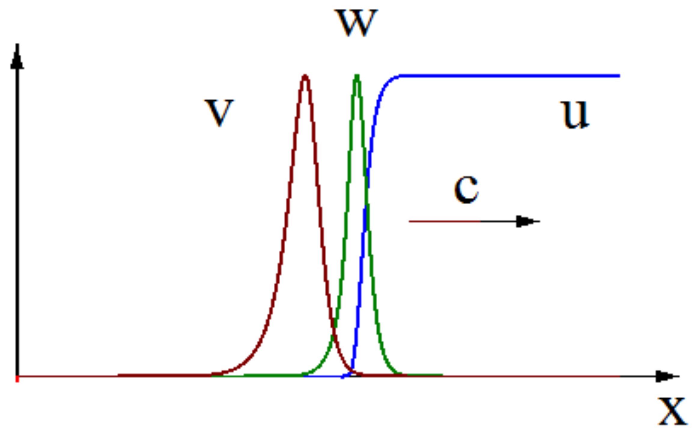
Experimental data and previous modeling show [10] that infection spreads in cell cultures as a reaction-diffusion wave (Figure 1). In order to study this solution, we consider a system of Equations (11)–(13) on the whole axis, and set $U(x,t)=u(x-ct),I(x,t)=w(x-ct),V(x,t)=v(x-ct)$, where c is the wave speed. Then we obtain the following system of equations:

$$-c{u}^{\prime }=-auv,$$

(14)

$$-c{w}^{\prime }=auv-\beta w,$$

(15)

$$-c{v}^{\prime }=D{v}^{″}+bw-\sigma v,$$

(16)

where primes denote the derivatives with respect to the variable $\xi =x-ct$. We are interested in the solution of this system of equations with the following limits at infinity:

$$u(-\infty )=u_f,u(\infty )=u_0,w(\pm \infty )=0,v(\pm \infty )=0.$$

(17)

In order to determine unknown value $u_f$, we proceed as in the previous section. From Equation (14), we obtain

$$cln\frac{u_0}{u_f}=a{\int }_{-\infty }^{\infty }v\left(x\right)dx,$$

(18)

taking a sum of (14), (15) and integrating:

$$c(u_0-u_f)=\beta {\int }_{-\infty }^{\infty }w\left(x\right)dx,$$

(19)

and from (16):

$$b{\int }_{-\infty }^{\infty }w\left(x\right)dx=\sigma {\int }_{-\infty }^{\infty }v\left(x\right)dx.$$

(20)

Excluding the integrals from Equations (18)–(20), we obtain the equation

$$R_v(\omega -1)=ln\omega ,$$

(21)

with respect to $\omega =u_f/u_0$. Equation (21) has a solution $\omega$ in the interval $0<\omega <1$ if and only if $R_v>1$. Thus, we obtain the following theorem.

Theorem 1.

Inequality $R_v>1$ provides a necessary condition for the existence of a positive solution of problem (14)–(17). In this case, the final value $u_f$ can be found from Equation (21), and the total viral load

$$V_X\equiv {\int }_{-\infty }^{\infty }v\left(x\right)dx=-\frac{c}{a}ln\omega .$$

Let us note that the notion of total viral load $V_X$ here is different from $V_T$ in the previous section. Here it signifies the total viral concentration in cell culture at any moment of time, while before it was the total viral load with respect to time (without space distribution). Furthermore, $V_X$ depends on the wave speed c, which is not yet found.

2.2.2. Model with Time Delay

In the model with time delay, Equation (13) is replaced by the equation

$$\frac{\partial V(x,t)}{\partial t}=D\frac{{\partial }^{2}V(x,t)}{\partial x^2}+bI(x,t-\tau )-\sigma V(x,t),$$

(22)

and Equation (16) by the equation

$$-c{v}^{\prime }\left(\xi \right)=D{v}^{″}\left(\xi \right)+bw(\xi +c\tau )-\sigma v\left(\xi \right).$$

(23)

Clearly, integration of this equation gives (20), and all conclusions above remain applicable for this case.

2.2.3. Minimal Wave Speed

In order to determine the wave speed, we will use the linearization method widely used for monostable reaction-diffusion equations beginning from the KPP work [12]. The idea of the method consists to consider the system linearized at infinity and to find the minimal wave speed $c_{*}$ for which this system has a positive decreasing solution. Thus, instead of Equations (15) and (16) we consider the equations

$$c{w}^{\prime }+a{u}_{0}v-\beta w=0,$$

(24)

$$D{v}^{″}+c{v}^{\prime }+bw(\xi +c\tau )-\sigma v=0,$$

(25)

where $u\left(\xi \right)$ is replaced by its value $u_0$ at infinity. We look for a solution of this system in the form

$$w\left(\xi \right)=p{e}^{-\lambda \xi },v\left(\xi \right)=q{e}^{-\lambda \xi }$$

with some positive numbers $p,q$ and $\lambda$. Substituting these expressions into Equations (24) and (25) and excluding p and q, we obtain the following equation with respect to $\lambda$:

$$D{\lambda }^2-c\lambda -\sigma +\frac{ab{u}_0}{c\lambda +\beta }=0.$$

We need to find a minimal positive value of c for which this equation has a positive solution. Set $\mu =\lambda c$. Then from the last equation we find

$$c^2=F\left(\mu \right),F\left(\mu \right)=\frac{D{\mu }^2(\mu +\beta )e^{\mu \tau }}{(\mu +\sigma )(\mu +\beta )e^{\mu \tau }-ab{u}_0}.$$

Under the condition $R_v>1$, that is, $\sigma \beta <ab{u}_0$, function $F\left(\mu \right)$ becomes negative for small positive $\mu$ and tends to $-\infty$ as $\mu \nearrow {\mu }_0$ for a positive ${\mu }_0$ for which the denominator vanish. Therefore, $F\left(\mu \right)>0$ for $\mu >{\mu }_0$, $F\left(\mu \right)$ decreases in some interval ${\mu }_0<\mu <{\mu }_{*}$ and increases for $\mu >{\mu }_{*}$. Hence, this function has a minimum for $\mu >{\mu }_0$ reached at $\mu ={\mu }_{*}$. Set

$$c_{*}^2=\underset{\mu >{\mu }_0}{min}F\left(\mu \right).$$

(26)

This equality provides the minimal wave speed found by the linearization method, and $\lambda ={\mu }_{*}/c_{*}$. Let us note that, in general, this method gives an estimate of the minimal wave speed $c_0$ from below, $c_0\ge c_{*}$. In some cases, it can be proved that $c_0=c_{*}$. This question is discussed in the next paragraph. Having found the wave speed, we can determine the total viral load $V_X$ in Theorem 1.

2.2.4. Wave Existence

If $\beta =0$, then we can reduce system (11)–(13) to a system of two equations. Indeed, taking a sum of Equations (11) and (12), we conclude that $U(x,t)+I(x,t)=U_0$, and the variable U can be excluded:

$$\frac{\partial I}{\partial t}=a(U_0-I)V-\beta I,$$

(27)

$$\frac{\partial V}{\partial t}=D\frac{{\partial }^{2}V}{\partial x^2}+b{I}_{\tau }-\sigma V.$$

(28)

This is a monotone system of equations for which it is possible to apply the maximum principle and various methods based on it. Existence of wave for this system is proved in [10] for all $c\ge c_0$ for the values of $\tau$ limited from above.

Thus, $c_0=c_{*}$ for $\beta =0$. If $\beta >0$, this equality is verified in numerical simulations [10]. Knowing the value of speed, we can construct an approximate solution in the following way. Consider system (15), (16) with $u=u_0$ for $\xi >0$ and $u=u_f$ for $\xi <0$. Then we find the wave speed $c_{*}$ and solution $w\left(\xi \right)$, $v\left(\xi \right)$ for $\xi >0$ as described in the previous paragraph. Let us note that this solution contains one unknown constant since there is a single relation between p and q. Next, we have a linear system for $\xi <0$ with a given value $c=c_{*}$. We can find its solution, and it depends on two unknown constants. These three constants can be determined from the continuity conditions at $\xi =0$: $w(-0)=w(+0),v(-0)=v(+0),v^{\prime }(-0)=v^{\prime }(+0)$. These calculations are quite cumbersome, and we do not present them here.

3. Viral Infection with Mutation

We will now consider the case where the first virus can mutate in another one. We consider the system of equations

$$\frac{\partial U}{\partial t}=-a_{1}U{V}_1-a_{2}U{V}_2,$$

(29)

$$\frac{\partial I_1}{\partial t}=a_{1}U{V}_1-{\beta }_1{I}_1,$$

(30)

$$\frac{\partial I_2}{\partial t}=a_{2}U{V}_2-{\beta }_2{I}_2,$$

(31)

$$\frac{\partial V_1}{\partial t}=D_1\frac{{\partial }^2{V}_1}{\partial x^2}+b_1{I_1}_{{\tau }_1}-{\sigma }_1{V}_1,$$

(32)

$$\frac{\partial V_2}{\partial t}=D_2\frac{{\partial }^2{V}_2}{\partial x^2}+ϵ{I_1}_{{\tau }_1}+b_2{I_2}_{{\tau }_2}-{\sigma }_2{V}_2$$

(33)

describing two viruses $V_1$ and $V_2$ in cell culture. Here U is the concentration of uninfected cells, $I_1$ of infected cells by virus $V_1$ and $I_2$ by virus $V_2$, $I_{{\tau }_1}\left(x\right)=I(x,t-{\tau }_1)$, $I_{{\tau }_2}\left(x\right)=I(x,t-{\tau }_2)$, $ϵ$ is the mutation rate which shows that cells infected by virus $V_1$ can produce virus $V_2$.

3.1. Reduction to the One-Virus Model

System (37)–(39) can be reduced to the one-virus model by setting $I_1=0,V_1=0$ or $I_2=0,V_2=0$. We are interested in the case where all components of the solution are positive. Under the assumptions ${\beta }_1={\beta }_2$, ${\sigma }_1={\sigma }_2$, $D_1=D_2$, ${\tau }_1={\tau }_2$, we look for the solution of system (29)–(33) in the form $I_2(x,t)=k_1{I}_1(x,t)$, $V_2(x,t)=k_2{V}_1(x,t)$. Then we rewrite Equations (31) and (33) as follows:

$$\frac{\partial I_1}{\partial t}=\frac{a_2{k}_2}{k_1}U{V}_1-{\beta }_1{I}_1,$$

(34)

$$\frac{\partial V_1}{\partial t}=D_1\frac{{\partial }^2{V}_1}{\partial x^2}+\frac{ϵ}{k_2}{I_1}_{{\tau }_1}+\frac{b_2{k}_1}{k_2}{I}_1{\tau }_1-{\sigma }_1{V}_1.$$

(35)

Comparing these equations with Equations (30) and (32), we conclude that

$$\frac{a_2{k}_2}{k_1}=a_1,\frac{ϵ+b_2{k}_1}{k_2}=b_1.$$

Hence,

$$k_1=\frac{ϵa_2}{a_1{b}_1-a_2{b}_2},k_2=\frac{ϵa_1}{a_1{b}_1-a_2{b}_2}.$$

(36)

Since we look for positive solutions, that is $k_1,k_2>0$, then we should impose the condition $a_1{b}_1>a_2{b}_2$.

Set $I=I_1+I_2=(1+k_1)I_1$, $V=V_1+V_2=(1+k_2)V_1$. Then we can write Equation (29), sum of Equations (30) and (31), and of Equations (32) and (33) as follows:

$$\frac{\partial U}{\partial t}=-aUV,$$

(37)

$$\frac{\partial I}{\partial t}=aUV-\beta I,$$

(38)

$$\frac{\partial V}{\partial t}=D\frac{{\partial }^{2}V}{\partial x^2}+b{I}_{{\tau }_1}-\sigma V,$$

(39)

where $\beta ={\beta }_1$, $\sigma ={\sigma }_1$, $D=D_1$,

$$a=\frac{a_1+a_2{k}_2}{1+k_2},b=\frac{ϵ+b_1+b_2{k}_1}{1+k_1},$$

where $k_1$ an $k_2$ are given by equalities (36). Hence, we obtain system (11)–(13) (or (22) in the case of time delay). We can formulate the following result.

Theorem 2.

Suppose that system (37)–(39) has a traveling wave solution $U(x,t)=u(x-ct),I(x,t)=w(x-ct),V(x,t)=v(x-ct)$, that is, solution of problem (14)–(17). If $ab{U}_0>\beta \sigma$ and $a_1{b}_1>a_2{b}_2$, then system (29)–(33) has a traveling wave solution with positive components $U(x,t)=u(x-ct),I_i(x,t)=w_i(x-ct),V_i(x,t)=v_i(x-ct)$, $i=1,2$ such that

$$w_1\left(\xi \right)=\frac{w\left(\xi \right)}{1+k_1},w_2\left(\xi \right)=\frac{k_{1}w\left(\xi \right)}{1+k_1},v_1\left(\xi \right)=\frac{v\left(\xi \right)}{1+k_2},v_2\left(\xi \right)=\frac{k_{2}v\left(\xi \right)}{1+k_2}.$$

(40)

This theorem allows us to apply to system (29)–(33) the results of the previous section obtained for system (11)–(13) on wave existence and speed of propagation.

Choice between Three Solutions

System (29)–(33) can have one-virus solutions for which $I_1=0,V_1=0$ or $I_2=0,V_2=0$, and two-virus solution for which all components are positive. Conditions $a_i{b}_i{U}_0>{\beta }_i{\sigma }_i$ and the results of the previous section provide the existence of the first-virus solution for $i=1$ and of the second-virus solution for $i=2$. Conditions of the existence of two-virus solution are provided by Theorem 2. If these conditions are not satisfied, we can expect that the two-virus solution does not exist, though Theorem 2 does not state this non-existence result. It is confirmed by the results of numerical simulations. Analytical values of wave speed coincide with the wave speed in numerical simulations.

3.2. Method of Linearization

Reduction to the one-virus model is applied above under the assumptions $D_1=D_2$, ${\beta }_1={\beta }_2$, ${\sigma }_1={\sigma }_2$, ${\tau }_1={\tau }_2$. If these conditions are not satisfied, we use the method of linearization to determine different regimes of infection spreading. We search solutions of system (29)–(33) in the form $U(x,t)=u(x-ct),I_1(x,t)=w_1(x-ct),I_2(x,t)=w_2(x-ct),V_1(x,t)=v_1(x-ct),V_2(x,t)=v_2(x-ct)$. Then,

$$c{u}^{\prime }-a_{1}u{v}_1-a_{2}u{v}_2=0,$$

(41)

$$c{w}_1^{\prime }+a_{1}u{v}_1-{\beta }_1{w}_1=0,$$

(42)

$$c{w}_2^{\prime }+a_{2}u{v}_2-{\beta }_2{w}_2=0,$$

(43)

$$D_1{v}_1^{″}+c{v}_1^{\prime }+b_1{w}_1(\xi +c{\tau }_1)-{\sigma }_1{v}_1=0,$$

(44)

$$D_2{v}_2^{″}+c{v}_2^{\prime }+ϵw_1(\xi +c{\tau }_1)+b_2{w}_2(\xi +c{\tau }_2)-\sigma v_2=0.$$

(45)

Set $u=u_0$,

$$v_1\left(x\right)=p_1{e}^{-\lambda x},v_2\left(x\right)=p_2{e}^{-\lambda x},w_1\left(x\right)=q_1{e}^{-\lambda x},w_2\left(x\right)=q_2{e}^{-\lambda x}.$$

Then,

$$p_1=\frac{\lambda c+{\beta }_1}{a_1{u}_0}{q}_1,p_2=\frac{\lambda c+{\beta }_2}{a_2{u}_0}{q}_2,$$

(46)

$$(D_1{\lambda }^2-c\lambda -\sigma )p_1+b_1{q}_1{e}^{-\lambda c{\tau }_1}=0,$$

(47)

$$(D_2{\lambda }^2-c\lambda -\sigma )p_2+ϵq_1{e}^{-\lambda c{\tau }_1}+b_2{q}_2{e}^{-\lambda c{\tau }_2}=0.$$

(48)

After straightforward calculations, we obtain

$$(D_1{\lambda }^2-c\lambda -\sigma )(c\lambda +{\beta }_1)e^{\lambda c{\tau }_1}{q}_1=-b_1{a}_1{u}_0{q}_1,$$

(49)

$$((D_2{\lambda }^2-c\lambda -\sigma )(\lambda c+{\beta }_2)+b_2{a}_2{u}_0{e}^{-\lambda c{\tau }_2})q_2+ϵa_2{u}_0{e}^{-\lambda c{\tau }_1}{q}_1=0.$$

(50)

If $q_1\ne 0$, then we deduce from (49) that

$$(D_1{\lambda }^2-c\lambda -\sigma )(\lambda c+{\beta }_1)e^{\lambda c{\tau }_1}=-a_1{u}_0{b}_1.$$

(51)

Set $\mu =c\lambda$. Then from the previous equality

$$\left(D_1\frac{{\mu }^2}{c^2}-\mu -\sigma \right)(\mu +{\beta }_1)e^{\mu {\tau }_1}=-a_1{u}_0{b}_1.$$

The wave speed $c_0$ is given by the equality

$$c_0^2=\underset{\mu >0}{min}F\left(\mu \right),F\left(\mu \right)=\frac{D_1{\mu }^2(\mu +{\beta }_1)e^{\mu {\tau }_1}}{(\mu +\sigma )(\mu +{\beta }_1)e^{\mu {\tau }_1}-b_1{a}_1{u}_0}.$$

(52)

In the particular case $D_1=D_2(=D)$, ${\tau }_1={\tau }_2(=\tau )$, ${\beta }_1={\beta }_2(=\beta )$, we obtained from (50) and (51), (46):

$$\frac{q_2}{q_1}=\frac{ϵa_2}{b_1{a}_1-b_2{a}_2},\frac{p_2}{p_1}=\frac{a_1}{a_2}\frac{q_2}{q_1}.$$

(53)

If $q_1=0$, then we have from (50)

$$((D_2{\lambda }^2-c\lambda -\sigma )(\lambda c+{\beta }_2)+b_2{a}_2{u}_0{e}^{-\lambda c{\tau }_2})q_2=0.$$

(54)

Then,

$$(D_2{\lambda }^2-c\lambda -\sigma )(\lambda c+{\beta }_2)e^{\lambda c{\tau }_2}=-b_2{a}_2{u}_0$$

(55)

Set $\mu =\lambda c$. The wave speed $c_0$ is given by the equality:

$$c_0^2=\underset{\mu >0}{min}\frac{D_2{\mu }^2(\mu +{\beta }_2)e^{\mu {\tau }_2}}{(\mu +\sigma )(\mu +{\beta }_2)e^{\mu {\tau }_2}-b_2{a}_2{u}_0}.$$

(56)

It is similar to the previous one but with the parameters characterizing the second virus.

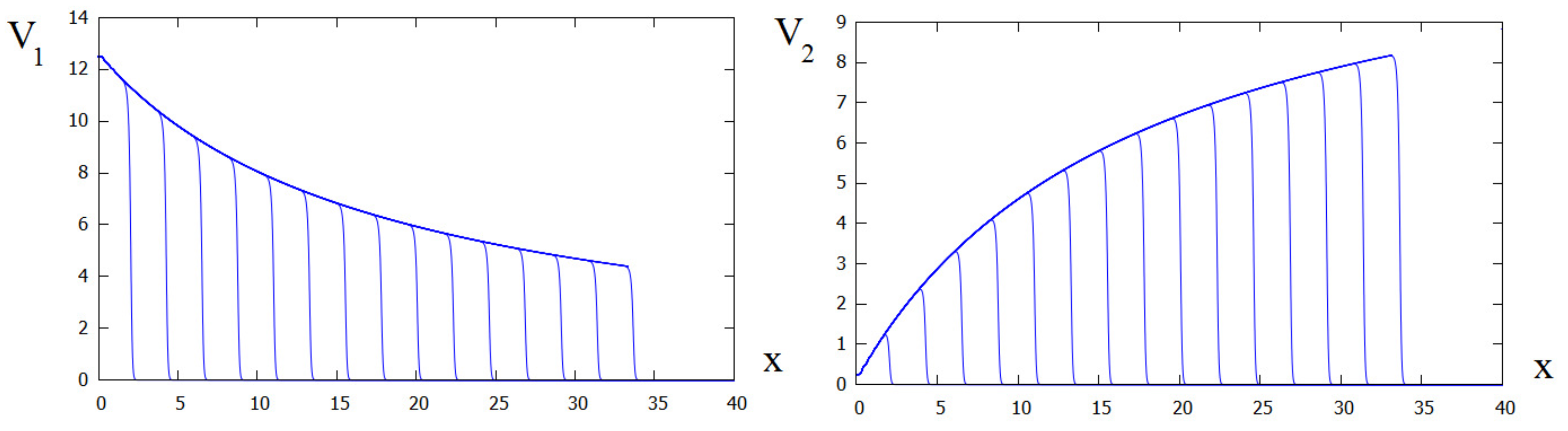
From (53) we can conclude that a positive solution exists if $a_1{b}_1>a_2{b}_2$, that is, replication of the first virus is faster than of the second one. This condition appears also in Theorem 1. In the case of equality, the first virus is gradually replaced by the second one due to the mutation process (Figure 2). If the inequality is opposite, the first virus vanishes faster since its replication is slower. We will return to this question in the next section.

3.3. Multiple Mutations and Coinfections

Generic model of virus mutation and coinfections can be written as follows:

$$\frac{\partial U}{\partial t}=-U\sum _{i=1}^n{a}_i{V}_i,$$

(57)

$$\frac{\partial I_i}{\partial t}=a_{i}U{V}_i-{\beta }_i{I}_i,i=1,...,n,$$

(58)

$$\frac{\partial V_i}{\partial t}=D_i\frac{{\partial }^2{V}_i}{\partial x^2}+\sum _{j=1}^n{b}_{ij}{I}_j-{\sigma }_i{V}_i,i=1,...,n.$$

(59)

The coefficient $b_{ij}$ (positive or negative) show that viruses can promote or downregulate replication of other viruses in the case of coinfection. As before, under certain conditions on parameters, we can set $I_i=p_{i}I$, $V_i=q_{i}V$, and reduce this system of equations to the one-virus model. In the case of negative coefficients $b_{ij}$ the positiveness of solution in Equation (59) does not directly follow from the equation, and it should be controlled.

4. Different Stages of Infection Progression

4.1. Single Virus

In the previous sections, we have studied reaction-diffusion waves of infection spreading in cell culture. The solution of the initial boundary value problem approaches the wave after the initial transient period. However, this initial period cannot be neglected in the investigation of viral infection since it determines further infection progression. It is particularly important from the point of view of interaction with the immune response, though we do not consider it in this work (see [13,14,15]).

In order to describe analytically the initial stage of infection development, instead of system (11)–(13), we consider the system

$$\frac{\partial U}{\partial t}=-aUV,$$

(60)

$$\frac{\partial I}{\partial t}=a{U}_{0}V-\beta I,$$

(61)

$$\frac{\partial V}{\partial t}=D\frac{{\partial }^{2}V}{\partial x^2}+b{I}_{\tau }-\sigma V,$$

(62)

where we replaced U by $U_0$ in Equation (61). This means that we neglect the depletion of uninfected cells in virus replication. This is a linear system which can be further simplified if we integrate the last two equations. In order to compare the results with the numerical simulations, we consider this system in a bounded interval $0<x<L$ with the boundary conditions

$$x=0,L:\frac{\partial V}{\partial x}=0.$$

(63)

Using the notation $J\left(t\right)={\int }_0^{L}I(x,t)dx$, $W\left(t\right)={\int }_0^{L}V(x,t)dx$, we obtain the delay differential system of equations

$$\frac{dJ}{dt}=a{U}_{0}W-\beta J,$$

(64)

$$\frac{dW}{dt}=b{J}_{\tau }-\sigma W$$

(65)

with the initial condition

$$J\left(t\right)=0,-\tau \le t\le 0,W\left(0\right)=W_0={\int }_0^{L}V(x,0)dx.$$

(66)

This system can be solved analytically. We restrict ourselves here to the two time intervals, $t\in [0,\tau )$:

$$J\left(t\right)=\frac{a{U}_0{W}_0}{-\beta +\sigma }(e^{-\beta t}-e^{-\sigma t}),W\left(t\right)=W_0{e}^{-\sigma t},$$

(67)

and $t\in [\tau ,2\tau )$:

$$W\left(t\right)=W_0{e}^{-\sigma t}+\frac{ab{U}_0{W}_0}{{(\beta -\sigma )}^2}\left[e^{-\beta (t-\tau )}(1+e^{h\left(t\right)}(-1+h\left(t\right)))\right],$$

$$J\left(t\right)=\frac{a{U}_0{W}_0}{(\beta -\sigma )}(e^{-\sigma t}-e^{-\beta t})+\frac{a^{2}b{U}_0^2{W}_0}{{(\beta -\sigma )}^3}\left(e^{-\sigma (t-\tau )}(-2+h\left(t\right)+e^{-h\left(t\right)}(2+h\left(t\right)))\right),$$

where $h\left(t\right)=(\beta -\sigma )(t-\tau )$, used for the comparison with the numerical simulations.

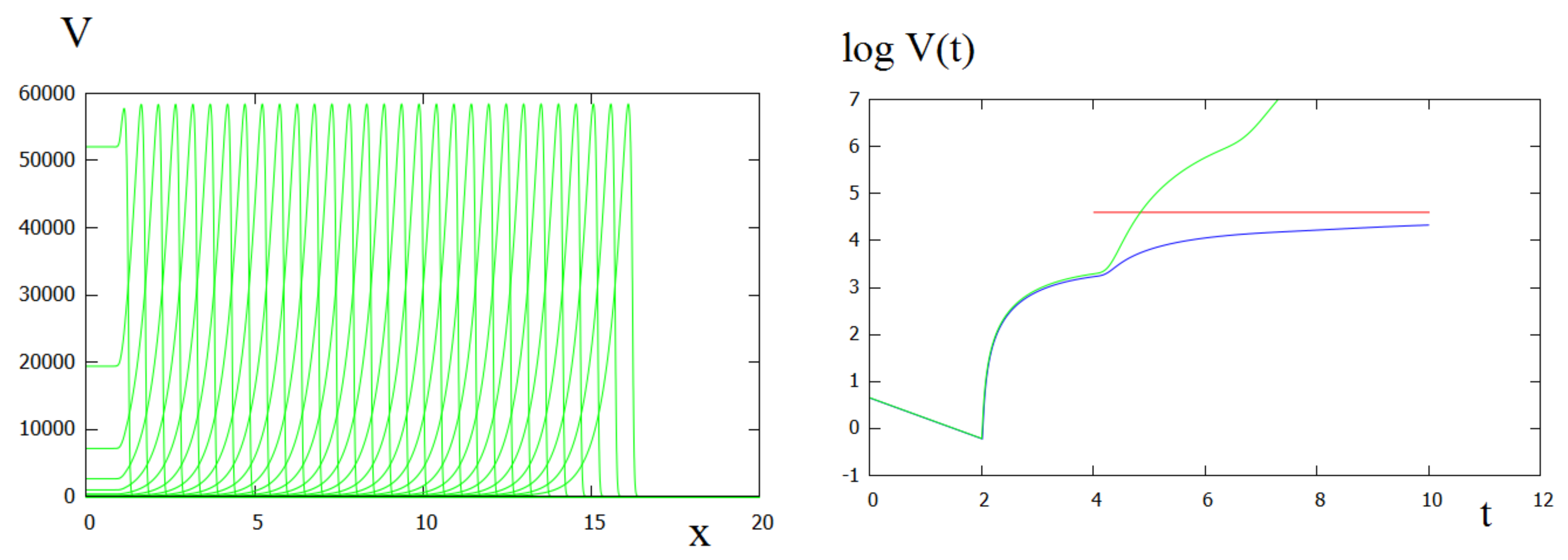
Figure 3 (left) shows the virus concentration distribution in consecutive moments of time with time difference between them equal 1 h. Let us note that since the length of the space interval is large and the diffusion coefficient is small, the descending part of the function V(x,t) looks steep in the graphical representation. It is smoother in Figure 4 and even more in Figure 1. Beyond the graphical representation, important question is about numerical accuracy. This descending part of solution contains about 130 discretization points, and the accuracy of the solution is verified.

The right panel of Figure 3 illustrates how the total viral load (the integral of virus concentration with respect to the whole space interval) changes in time. The total viral load is determined in direct numerical simulations of the space-dependent problem (11)–(13) and by two approximate analytical methods. The first one is based on solution of linear ODE (64), (65). It is applicable for a relatively small time ($t<4$). The second analytical approximation uses Theorem 1 and the formula for the wave speed that allows us to determine the viral load in the propagating wave for t large enough.

4.2. Virus Mutation and Competition

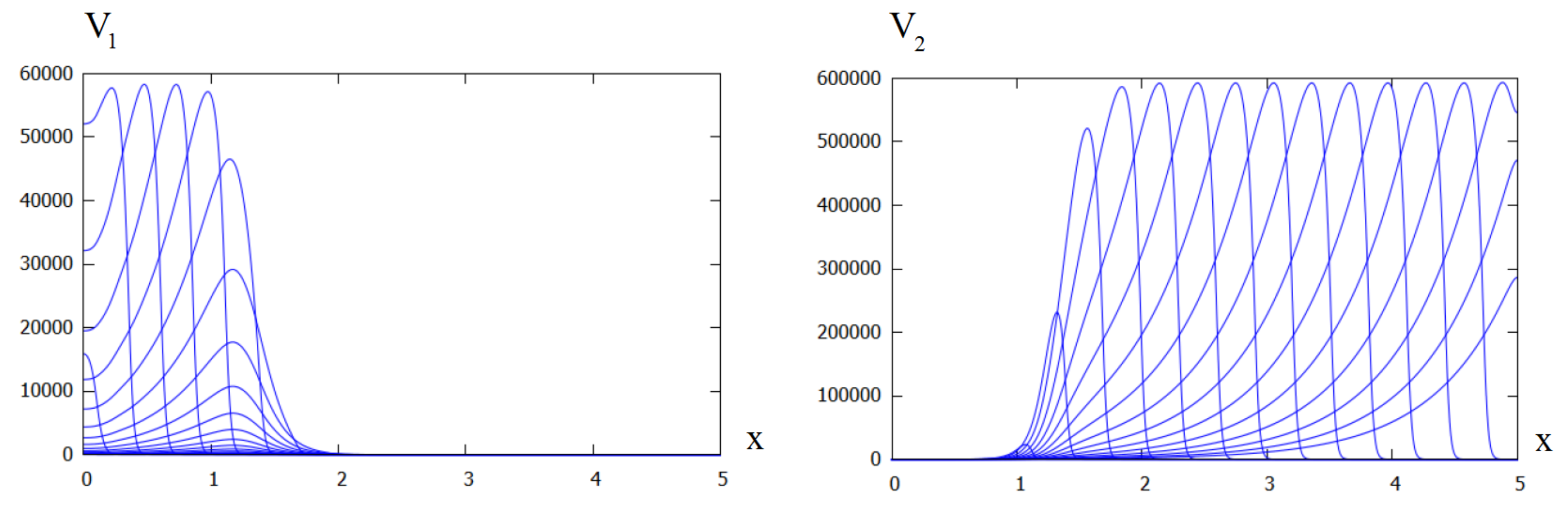
In Section 3, we have established conditions of the coexistence of two viruses in cell culture. If these conditions are not satisfied, and the new variant replicates faster, it will eliminate the first one (Figure 4).

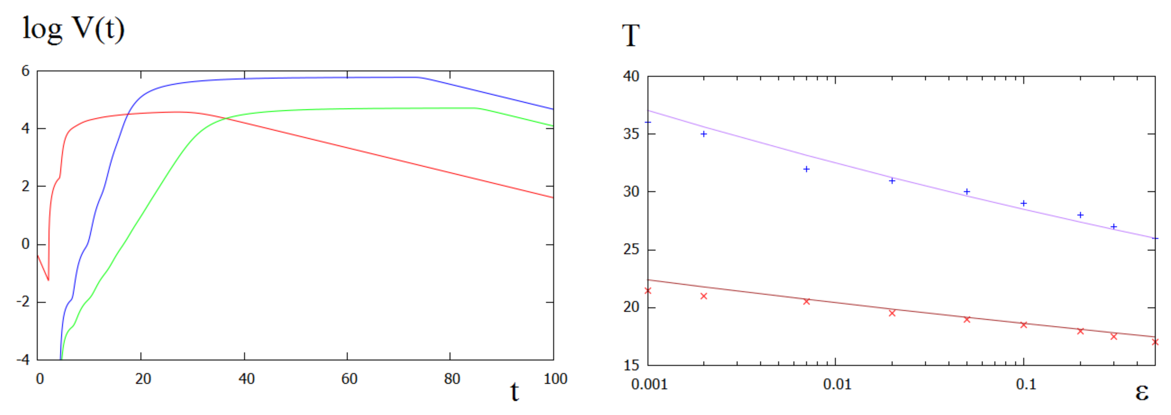
Analysis of the total viral load (Figure 5) shows that there are four stages of infection progression in this case instead of the three stages observed previously. After the infection decay and explosive growth, the distribution of the first virus reaches its bell-shape form and propagates along the culture. At the same time, the total viral load of the second virus variant exponentially grows. When it is reaches its maximum, the first viral load begins its exponential decay.

Denote by T the transition time defined as the moment of time at which $V_2\left(t\right)$ reaches 90% of its maximal value. Transition time depends on the mutation rate and on the replication rates determined by the parameters $a_i,b_i$, $i=1,2$ (Figure 5, right). As it can be expected, T is larger for small $ϵ$, and it decreases if the replication rate of the second virus increases. The dependence of T on $ϵ$ is well approximated by the function $p/{ϵ}^q$ with some fitted values of p and q. Let us note that the for these values of q, the dependence of the transition time on $ϵ$ is weak. Extrapolating the curves using the analytical approximation, we can see that decreasing the mutation rate by ${10}^6$ increases the transition time only about twice.

4.3. Values of Parameters

The values of parameters for the single variant were determined in [10] by fitting the experimental data on the variation of viral load in time. Parameter estimation begins with the first stage of infection development during which virus is not yet reproduced by the infected cells, and its concentration exponentially decays. Duration of this stage and the decay rate allow us to uniquely determine parameters $\tau$ and $\sigma$ by comparison with the total viral load in the experimental data. The next stage is characterized by explosive virus production with the maximum of the total viral load determined by the parameter b. At the same time, parameter a is chosen for the best fit of the growth curve. Finally, the third stage of infection development corresponds to its propagation in cell culture as a reaction-diffusion wave. The total viral load remains constant for $\beta =0$, and it has a slow growth for a positive $\beta$, also determined by comparison with the total viral load in the experiment. Virus diffusion coefficient D is estimated from the literature. Let us recall the dimensions of the main parameters: $\left[L\right]\sim$cm, [time] ∼ hours, $\left[\tau \right]\sim$ hours, $\left[\sigma \right]\sim$ 1/hour, $\left[D\right]\sim$cm${}^2$/hour.

The replication rate for the second virus (constants $a_2$, $b_2$ versus $a_1$, $b_1$) is taken in the same range or larger than that for the first virus. In order to evaluate the mutation rate $ϵ$, let us note that the rate of mutations of RNA viruses is from ${10}^{-6}$ to ${10}^{-4}$ per base per generation. Taking into account that only from $0.001$ to $0.01$ viruses represent plaque forming units, we estimate the probability of a given mutation during one virus replication of the order of ${10}^{-9}$ to ${10}^{-6}$. The virus replication rate with respect to a single cell in the model is given by the constant $b_1=8\times {10}^4$. Multiplied by the probability determined above, we obtain the value of $ϵ$ in the range from ${10}^{-4}$ to ${10}^{-1}$. Further, we can reasonably assume that viruses of the same size have close diffusion coefficients. In particular, this is the case of two variants of the same virus. Therefore, we take the same values of diffusion coefficient for both viruses.

5. Discussion

Multiplicity of virus assays represent conventional tests for the assessment of virus virulence and other properties [3,5]. In a previous work [10], we have shown that infection spreading in cell culture can be described by a reaction-diffusion system with time delay. Three stages of infection progression were identified: virus decay, explosive growth, wave propagation. In this work, we apply this modeling approach to study virus mutation during infection progression. This question has a particular importance in the context of the emergence of new virus variants in COVID-19 pandemic. In a simplified setting, without taking into account the influence of the immune response, we can model this process as infection progression in cell culture and analyze the conditions of the emergence of new virus strains.

We introduce in this work the notion of virus replication number $R_v$ (similar to the basic reproduction number in epidemiological models) and show that infection spreads in cell culture if this number calculated for the first virus is larger than 1. Furthermore, the total viral load can be expressed in terms of $R_v$.

If the first virus variant spreads in cell culture and it can give a new virus variant due to mutations, then the two virus can co-exist or the second virus can eliminate the first one. The condition of their coexistence is given by the inequality $a_1{b}_1>a_2{b}_2$. Taking into account that the coefficients $a_i$ characterize the rate of cell infection and the coefficients $b_i$ the rate of virus replication in the infected cells, their product $a_i{b}_i$ describes the total rate of virus production in cell culture. Hence, the two viruses coexist if the first one is produced faster than the second one. Otherwise, the second virus eliminates the first one.

The transition time from the first virus to the second virus depends on the mutation rate and on the replication rates. It is an important characterization of new variants since it shows whether they have enough time to develop in patients during the disease duration. The estimates of the transition time show that its dependence on the mutation rate is weak. Therefore, once new variant appears, it will rapidly replace the original one if it replicates faster, and the infected individual will become a career of the new variant.

This work is limited to the investigation of the emergence of new virus variants in the experimental setting of cell culture. The influence of the immune response on the infection mutation and spreading in the human organism will be considered in further works. However, some preliminary conclusions can be already done on the basis of the results of this work, in particular, about the action of vaccines on disease progression. In the case of SARS-CoV-2, the vaccine acts on virus spike preventing its penetration into the host cells. In the framework of the model, vaccine action can be described by decreasing the coefficient a. If it becomes small enough, such that the virus replication number $R_v$ is less than 1, then infection will not develop. If $R_v$ decreases but remains greater than 1, then infection will develop. However, infection spreading speed decreases. For the patients it signifies that disease symptoms are less severe.

References

- Czerkies, M.; Korwek, Z.; Prus, W.; Kochanczyk, M.; Jaruszewicz-Blonska, J.; Tudelska, K.; Blonski, S.; Kimmel, M.; Brasier, A.R.; Lipniacki, T. Cell fate in antiviral response arises in the crosstalk of IRF, NF-kB and JAK/STAT pathways. Nat. Commun. 2018, 9, 493. [Google Scholar] [CrossRef] [PubMed]
- Dykes, C.; Wang, J.; Jin, X.; Planelles, V.; An, D.S.; Tallo, A.; Huang, Y.; Wu, H.; Demeter, L.M. Evaluation of a multiple-cycle, recombinant virus, growth competition assay that uses flow cytometry to measure replication efficiency of human immunodeficiency virus type 1 in cell culture. J. Clin. Microbiol. 2006, 44, 1930–1943. [Google Scholar] [CrossRef] [PubMed] [Green Version]
- Jegouic, S.; Joffret, M.L.; Blanchard, C.; Riquet, F.B.; Perret, C.; Pelletier, I.; Colbere-Garapin, F.; Rakoto-Andrianarivelo, M.; Delpeyroux, F. Recombination between polioviruses and co-circulating coxsackie A viruses: Role in the emergence of pathogenic vaccine-derived polioviruses. PLoS Pathog. 2009, 5, e1000412. [Google Scholar] [CrossRef] [PubMed]
- Lindsay, S.M.; Timm, A.; Yin, J. A quantitative comet infection assay for influenza virus. J. Virol. Methods 2012, 179, 351–358. [Google Scholar] [CrossRef] [PubMed] [Green Version]
- Sims, A.C.; Baric, R.S.; Yount, B.; Burkett, S.E.; Collins, P.L.; Pickles, R.J. Severe acute respiratory syndrome coronavirus infection of human ciliated airway epithelia: Role of ciliated cells in viral spread in the conducting airways of the lungs. J. Virol. 2005, 79, 15511–15524. [Google Scholar] [CrossRef] [PubMed] [Green Version]
- Yin, J.; McCaskill, J.S. Replication of viruses in a growing plaque: A reaction-diffusion model. Biophys. J. 1992, 61, 1540–1549. [Google Scholar] [CrossRef]
- Holder, B.P.; Simon, P.; Liao, L.E.; Abed, Y.; Bouhy, X.; Beauchemin, C.A.; Boivin, G. Assessing the in vitro fitness of an Oseltamivir-resistant seasonal A/H1N1 influenza strain using a mathematical model. PLoS ONE 2011, 6, e14767. [Google Scholar] [CrossRef] [PubMed] [Green Version]
- Akpinar, F.; Inankur, B.; Yin, J. Spatial-temporal patterns of viral amplification and interference initiated by a single infected cell. J. Virol. 2016, 90, 7552–7566. [Google Scholar] [CrossRef] [PubMed] [Green Version]
- Rodriguez-Brenes, I.A.; Hofacre, A.; Fan, H.; Wodarz, D. Complex dynamics of virus spread from low infection multiplicities: Implications for the spread of oncolytic viruses. PLoS Comput. Biol. 2017, 13, e1005241. [Google Scholar] [CrossRef] [PubMed] [Green Version]
- Ait Mahiout, L.; Bessonov, N.; Kazmierczak, B.; Sadaka, G.; Volpert, V. Infection spreading in cell culture as a reaction-diffusion wave. EDP Sci. 2022. submitted. [Google Scholar]
- Hecht, F. New development in FreeFEM++. J. Numer. Math. 2012, 20, 251–256. [Google Scholar] [CrossRef]
- Kolmogorov, A.N.; Petrovskii, I.G.; Piskunov, N.S. Etude de l’quation de la chaleur avec croissance de la quantité de matière et son application à un problème biologique. Bull. Moskov. Gos. Univ. Mat. Mekh. 1937, 1, 1–25. [Google Scholar]
- Bessonov, N.; Bocharov, G.; Meyerhans, A.; Popov, V.; Volpert, V. Existence and Dynamics of Strains in a Nonlocal Reaction-Diffusion Model of Viral Evolution. SIAM J. Appl. Math. 2021, 81, 107–128. [Google Scholar] [CrossRef]
- Bocharov, G.; Meyerhans, A.; Bessonov, N.; Trofimchuk, S.; Volpert, V. Modelling the dynamics of virus infection and immune response in space and time. Int. J. Parallel Emergent Distrib. Syst. 2019, 34, 341–355. [Google Scholar] [CrossRef] [Green Version]
- Bocharov, G.; Meyerhans, A.; Bessonov, N.; Trofimchuk, S.; Volpert, V. Interplay between reaction and diffusion processes in governing the dynamics of virus infections. J. Theor. Biol. 2018, 457, 221–236. [Google Scholar] [CrossRef] [PubMed]
Figure 1.
A snapshot of numerical solution of system (11)–(13). Infection spreads as a reaction-diffusion wave with a speed c, . Note that here.
Figure 2.
Numerical simulations of system (29)–(33) in the case where . Both virus spread in the form of waves, but the concentration of the first virus slowly decreases while of the second virus increases. The values of parameters: .
Figure 3.
Left: virus distribution in consecutive moments of time (every 1 h). Right: total viral load (in the logarithmic scale) found as solution of system (64), (65) (green), of system (11)–(13) (blue) and by the formula in Theorem 1 (red). The values of parameters: .
Figure 4.
Distributions of (left) and (right) in numerical simulations of system (29)–(33). In the beginning of simulations, there is only the first virus variant. After some time, the second variant completely eliminate the first one. The values of parameters: .
Figure 5.
Left: (red) and (green) in the logarithmic scale for ; (blue) for . Right: transition time T as a function of mutation rate for (upper curve, crosses) and (lower curve, crosses). Smooth lines represent analytical approximation with the functions , (upper curve), (lower curve). The values of parameters: .
Publisher’s Note: MDPI stays neutral with regard to jurisdictional claims in published maps and institutional affiliations. |
© 2022 by the authors. Licensee MDPI, Basel, Switzerland. This article is an open access article distributed under the terms and conditions of the Creative Commons Attribution (CC BY) license (https://creativecommons.org/licenses/by/4.0/).
Share and Cite
MDPI and ACS Style
Ait Mahiout, L.; Kazmierczak, B.; Volpert, V. Viral Infection Spreading and Mutation in Cell Culture. Mathematics 2022, 10, 256. https://doi.org/10.3390/math10020256
AMA Style
Ait Mahiout L, Kazmierczak B, Volpert V. Viral Infection Spreading and Mutation in Cell Culture. Mathematics. 2022; 10(2):256. https://doi.org/10.3390/math10020256
Chicago/Turabian StyleAit Mahiout, Latifa, Bogdan Kazmierczak, and Vitaly Volpert. 2022. "Viral Infection Spreading and Mutation in Cell Culture" Mathematics 10, no. 2: 256. https://doi.org/10.3390/math10020256
Note that from the first issue of 2016, this journal uses article numbers instead of page numbers. See further details here.