
Bond-Graph-Based Approach to Teach PID and Sliding Mode Control in Mechatronics


Engineering Department, Faculty of Mechatronics, University of Debrecen, Egyetem tér 1, 4032 Debrecen, Hungary
*
Author to whom correspondence should be addressed.
Machines 2023, 11(10), 959; https://doi.org/10.3390/machines11100959
Submission received: 31 August 2023
/
Revised: 29 September 2023
/
Accepted: 12 October 2023
/
Published: 14 October 2023
(This article belongs to the Special Issue Control and Mechanical System Engineering)
Abstract
:The main contribution of this article is creating synergy between subjects; this means that students use the same graphical tool in several subjects. So far, the bond graph has not been used in control theory, but it is the “native language” of mechatronics engineers, so we would like to introduce it into the teaching of control theory. The bond graph method is proposed as a novel teaching method to teach mechatronics subjects in the paper. The bond graph is a graphical alternative to ordinary differential equations from a mathematical standpoint. Traditionally, control theory employs ordinary differential equations, as they are familiar to control theorists. However, mathematically, both approaches are equivalent but require a slightly different approach in their application. This article highlights the mathematical similarities between the two approaches while emphasizing the distinctions in graphical representation. Another contribution is that the PID and sliding mode controller are represented using the bond graph method. In the meantime, through the use of practical examples, we effectively illustrate how the same problem can be solved using either approach. In the training materials, the PID controller and an adaptive robust sliding mode controller (ARSMC) with the bond graph are utilized as examples to demonstrate synergy in mechatronics. Finally, we present proof that mechatronic engineers achieve superior outcomes when utilizing the bond graph approach, based on test results from undergraduate students.
1. Introduction
There is an increasing demand for the integration of control theory in everyday devices. The equipment contains more and more controllers than before, which makes control theory play a critical role in mechatronics engineering. Mechatronics is an interdisciplinary subject, including electronics, mechanical, and control theory [1]. Traditionally, control theory employs block diagrams, and block diagrams are derived from ordinary differential equations(ODEs). ODEs could be substituted by the bond graph from a mathematical point of view.
Mechatronics systems are defined as multidisciplinary engineering systems, combining precise mechanical engineering, electronic control, and intelligent software in a system framework that is utilized in product design and production processes [1]. Mechatronics engineering focuses on realistic problem solutions from a strong mathematical background standpoint because of the cross-subject characteristics [2]. Mechatronics subjects are interdisciplinary, which means the students need to master the knowledge of multiple subjects to fulfill the requirements of daily study [3]. Mechatronics engineering includes four components: mechanics, electronics, computers, and control methods. The more components involved, the more technologies and teaching methods [4]. The education of undergraduate mechatronics engineering should focus on fundamental knowledge, due to the critical role it plays [5]. After introducing the education aspect, from a robotics application point of view, mechatronics subjects need integration tools to achieve synergy since they contain multidisciplinary field knowledge [6,7]. Bond graph is proposed as an integration graphical tool to present the synergy in mechatronics engineering, and it has been proposed as the right choice for education students in modeling systems for decades [8]. The bond graph has been not only as an intelligent design support in the education monitoring system [9] but also as an interactive teaching modeling tool in bioengineering modeling and simulation [10]. According to the paper [11], mechatronics subjects require a series of operations such as analysis and assessment to draw students’ attention and accomplish multidisciplinary. It points out that students prefer a relaxed and visual teaching method to traditional teaching methods [12]. Therefore, this article uses a new teaching model in conjunction with traditional education and develops a suitable teaching model by analyzing and assessing students.
Bond graph is a graphical and visual tool to represent the energy flows in multiple domains [13], it could represent many fields not only the thermomechanical field [14], but also the mechatronics subject [15]. Besides applying simulation in multiple domains and system-level understanding, the bond graph deals with fault diagnosis in the industry field [16].
The bond graph has all the advantages of the visual representation. Visual representations such as graph illustrations and diagrams increased favorability with students [17]. The graph plays a pivotal role in various domains, and it is relevant for understanding and comprehending [18]. Research from Stanford University said that visual representations are not only for lower-level work but also for more advanced or abstract [19].
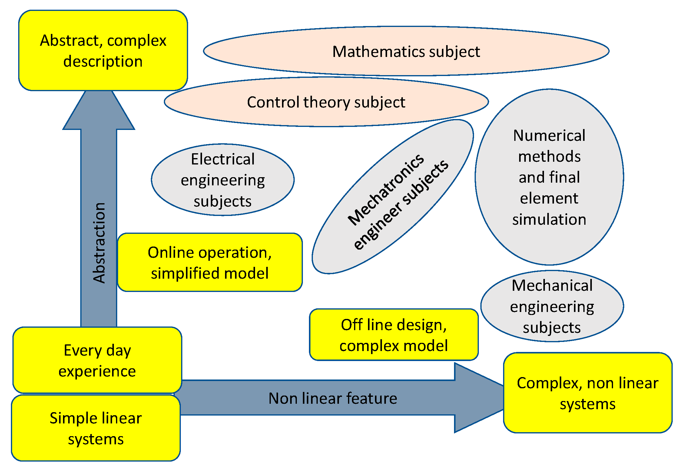
The proportional–integral–derivative (PID) controller is a classical linear controller [20,21,22] in control theory. The benefits of adaptive reference control of the model are essentially outlined in [23]. In control theory, there is no perfect controller; for example, the PID controller response is quick, but there is an obvious oscillating response before reaching the desired value as seen in the simulation [24]. Compared with the PID controller, the sliding mode controller is a type of discontinuous or nonlinear control approach [25], which provides nonlinearity in DC motor speed control [26]. The sliding mode controller is chosen as a teaching material because it requires high nonlinear features and high abstraction in the mechatronics engineering and control theory just as Figure 1 shows [27,28,29].
A simple conclusion can be derived from all the surveys above: the mechatronics subject is an interdisciplinary and complex subject for university students. And the task for teachers is to figure out an easier method to teach relevant subjects. The bond graph is proposed as the core method of mechatronics subjects, because of its power synergy function and comprehensive graphical language.
The core subject, ‘modeling and simulation’, integrates a high level of abstraction and non-linear features as shown in Figure 1. Students need to spend plenty of time studying mechatronics subjects using the traditional method. In this paper, a new teaching method, the bond graph method with a high accelerated learning curve is proposed for students to learn mechatronics subjects. It could help students learn and master the subject concepts quickly compared with the traditional mathematical method.
Compared with the traditional methodology, students can derive block diagrams directly from the bond graph without complex mathematical calculations. This comparison indicates that the bond graph method is a more straightforward approach to explaining system dynamics compared to the traditional mathematical method.
1.1. Motivation and Problem Statement
The bond graph is a powerful graphical tool in the control system. The demand for control theory in everyday devices is expanding, necessitating the involvement of not only dedicated control specialists but also a wider range of engineers to fully embrace control theory. However, it is essential to introduce an alternative teaching method to effectively engage non-specialists in understanding and applying control theory principles. The objective is to empower mechatronic engineers to extend their proficiency in mathematical modeling tools from mechatronics design to control system design.
From the mechatronics point of view, the DC motor with control is a good example since it has electrical and mechanical parts. From the control theory perspective, DC motor control is very simple since the generation of the magnetic field and generation of the torque can be controlled separately. We can assume that the magnetic field is constant, and we focus on the rotation of the motor. Three possible variables can be controlled: torque, angular velocity, and position angle.
The very basic controller type is the PID all textbooks on control start with. What is very new in this article is the bond graph description of the PID controller.
The sliding mode control (SMC) is selected as a little bit of an advanced control. It is popular in the field of motion control since the real system always consists of power electronics elements. The term ’power electronics’ refers to switching-mode transistors, making it a typical variable structure system. Sliding mode is a special operation mode of variable structure systems. The realization of a sliding mode controller is straightforward from an engineering standpoint; however, the mathematical description of the sliding mode requires highly sophisticated mathematical techniques [30]. Undergraduate students can write a simple code for sliding mode control even if they do not understand the whole and deep theoretical background.
The professor decided on the bond graph method as a practical graphical tool [31,32] for the modeling subject in the mechatronics engineering faculty University of Debrecen around 2015. First, the bond graph was introduced to MSc students in Control Theory subject, and later we introduced it in undergraduate Basics of Mechatronics (first semester) and Modelling and Simulation subject (fifth semester). According to the literature, PID and sliding mode controllers have not been represented using the bond graph before.
1.2. Structure of the Article
In this paper, the novel teaching method structure is as follows: the Section 2 introduces the simulation of the DC motor using the traditional method and the bond graph. Section 3 demonstrates the teaching methods to mechatronics undergraduate students using a PID controller. In Section 4, the paper proposed a simple sliding mode controller with a general target model and an adaptive robust sliding mode control with the real motor parameters as nonlinear-control teaching materials. The controllers and the model are simulated using the bond graph method. And, in the following section, the paper presents sample tests conducted on undergraduate students from the mechatronics department, at the University of Debrecen. The results are showcased in a chart format, providing evidence to support the claim that the bond graph method is an efficient and acceptable learning tool compared to the traditional mathematical method for mechatronics engineering students.
2. DC Electrical Machine Modeling
A DC motor is the demonstration model utilized as a teaching material in this course. The DC electrical machines are applied as a fundamental actuator model in undergraduate mechatronics engineering study. Most electrical machines can be simplified as DC electrical machines. As a result, DC electrical machines are commonly employed as actuation elements in industrial applications. The DC electrical machines are simple to model and analyze, making them ideal for educational purposes.
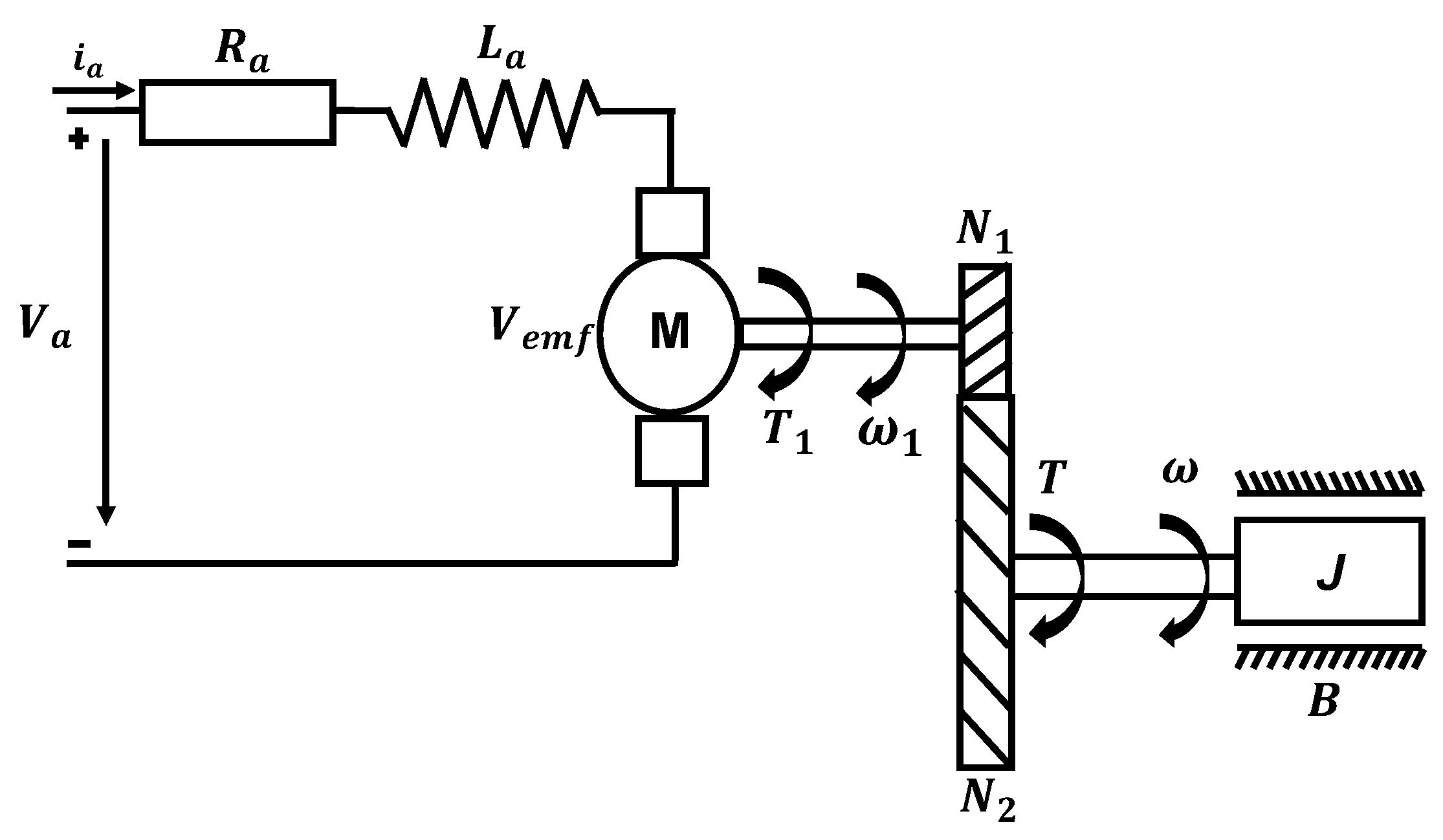
The electrical circuit on the left side is connected by a voltage resource, an inductor, and a resistor with a series connection. The mechanical side relates to a gearbox and winding with moments of inertia. An “ideal motor” connects electrical and mechanical parts in Figure 2. The ideal motor is modeled as a resistance, an inductor and back electromotive force.
An ideal gearbox with the ratio set to is added to the DC motor model for convenient simulation, where the torque and angular velocity relationship are , and .
2.1. DC Motor Modeling Using Ordinary Differential Equation (ODE)
A mathematical representation of the DC motor is shown in the following () and ().
where the left side of the rotor is the electrical part, the circuit consists of a resistor ; an inductor ; is the back electromotive force ; is the armature voltage; and donates the armature current of the electrical circuit. On the right side of the rotor, is the electromechanical torque generated by the motor, is the torque transform by gearbox, and denotes the load torque. (rad/s) shows the speed of the motor, (rad/s) donates the speed of the rotor, and represent the rotor inertia and the viscous friction of the DC motor electrical part. and represent the gyrator’s back EMF constant and motor constant, respectively.
The time constant is a critical parameter of the DC motor which could provide a rough estimate of DC motor response time; the step time of simulation should be shorter than the DC motor time constant. Electrical constant = = s = 0.106 .
The low pass filter time constant at the D-part in the PID controller is set to ; it has the same order as the electrical time constant of the motor. The rotor inertia and the mechanical time constant could derive the coefficient of viscous friction: 0.898 Nms/rad. And the torque constant is equal to the back EMF constant: 16.8 Vms/rad. DC motor and gear drive parameters are all based on the motor Maxon A-Max26 (1109961) and gear drive (110396) shown in Table 1 and Table 2.
2.2. Bond Graph Modeling in the Control Loop in Mechatronics Engineering
The mathematical methodology solution could be more difficult if the schematic is complex enough; in the meantime, the bond graph could prove an easier solution to solve the same question of the traditional method.
Our department uses the bond graph method to derive the block diagram rather than using the usual method. The bond graph may be constructed immediately by the schematic, obviating the steps of traditional formula analysis. The bond graph could merge two separate field systems. The DC electrical machine is an excellent example to demonstrate this principle.
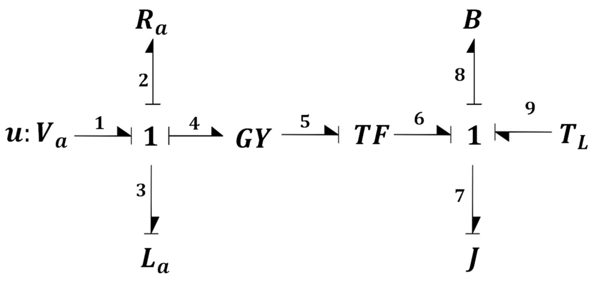
The bond graph of the DC motor is depicted in Figure 3. There are two parts to the bond graph. The electrical and mechanical parts are represented by two 1junctions, respectively. The gyrator connects two parts since the DC motor can convert one form of energy to another form of energy. TF represents the gearbox in the schematic because the energies’ form is the same as the gearbox. The numbers on the bond are the notation, which could help with visualization and calculation of the energies and flows.
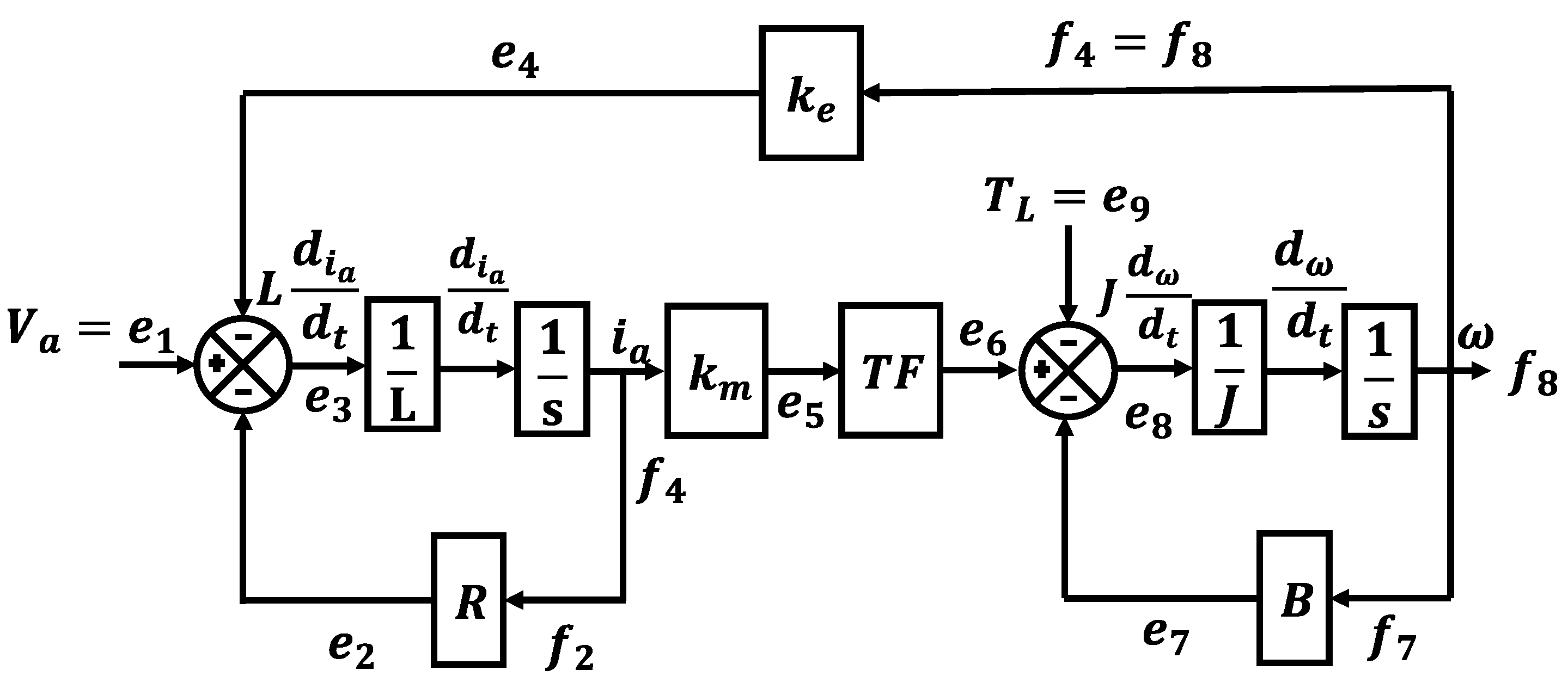
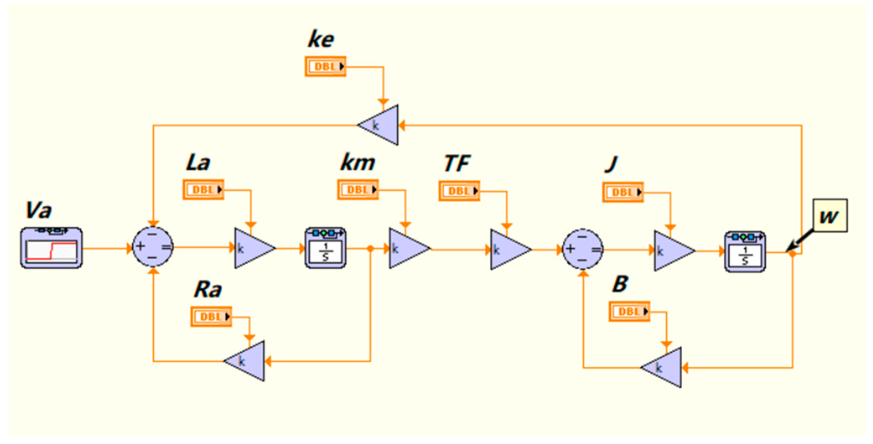
The block diagram can be derived from the bond graph method shown in Figure 4. It analyzes the directions of energies and flows instead of complex mathematical calculations. The bond graph method is much more acceptable than the traditional learning method for the students.
The relation of all the components is in the flowing: the first 1–junction represents the common flow energy; the common flow is the current of the electrical circuit. The calculation of the 1–junction is the effort energy: , the output of the first junction is . Then, the equation is . The same concept applies to the second 1–junction, . TF is the gearbox and the are the GY parameters.
The final goal of the “modeling and simulation” subject is to study the performance or methodology comparison from the simulation data. The simulation software is LabVIEW–2014, and the LabVIEW code could be generated from the block diagram above shown in Figure 5.
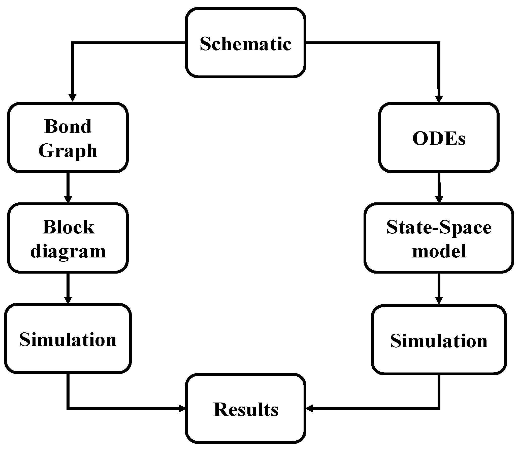
A comparison of the two methods is shown in Figure 6. The right side is the traditional mathematical method using the ordinary differential equation (ODE) and state-space to derive the block diagram. The bond graph method is proposed on the left side, the bond graph could be converted from the schematic directly, and the block diagram can be derived by analyzing the bond graph energies’ flow.
The two methods are essentially the same with minor differences in details. The block diagram derived from the bond graph can implicitly explain the directions of energy flows. The bond graph is an efficient method to derive the block diagram. It does not mean that the bond graph method is better than the ODE; the bond graph method could provide a clear relationship of the whole system from the graphical point of view in mechatronics engineering. It could represent multiple domains using the same graphical language, which could enhance the synergy in the mechatronics engineering subject.
3. Linear Control with the Bond Graph Method for Undergraduate Students
This paper not only presents new teaching methods for the students but also provides teaching strategies. The teaching strategy is to make the knowledge modular; in the meantime, it could train students to think by themselves when they face a new assignment by building the knowledge brick by brick.
Linear control is a fundamental control method in the control theory. A PID controller is a typical controller for the DC motor speed control in the linear controller domain.
Modular knowledge could be demonstrated using Figure 7. All the knowledge was taught to the students modularly; students could solve new tasks by integrating knowledge.
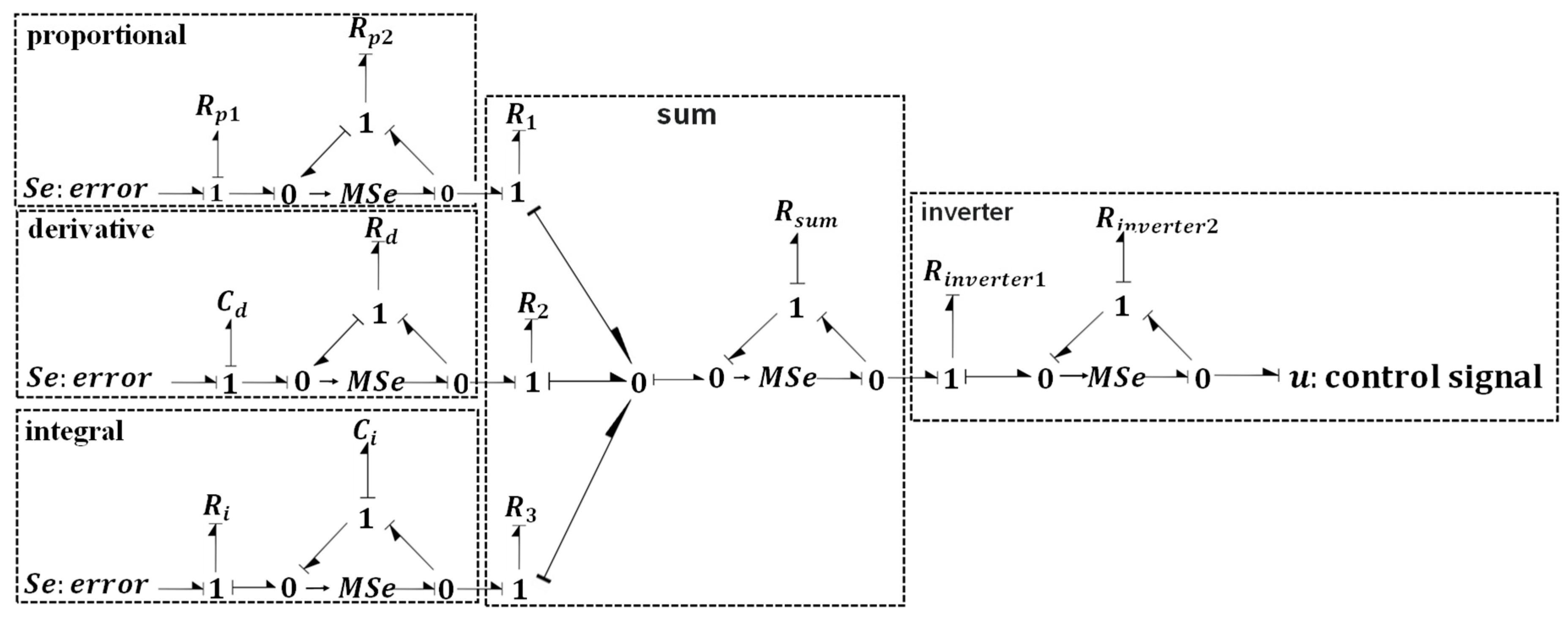
PID controller can be represented using the bond graph operational amplifiers separately. The bond graph of the PID controller contains an inverter operational amplifier, differential operational amplifier, and integral operational amplifier. The bond graph of the PID controller is shown in Figure 8.
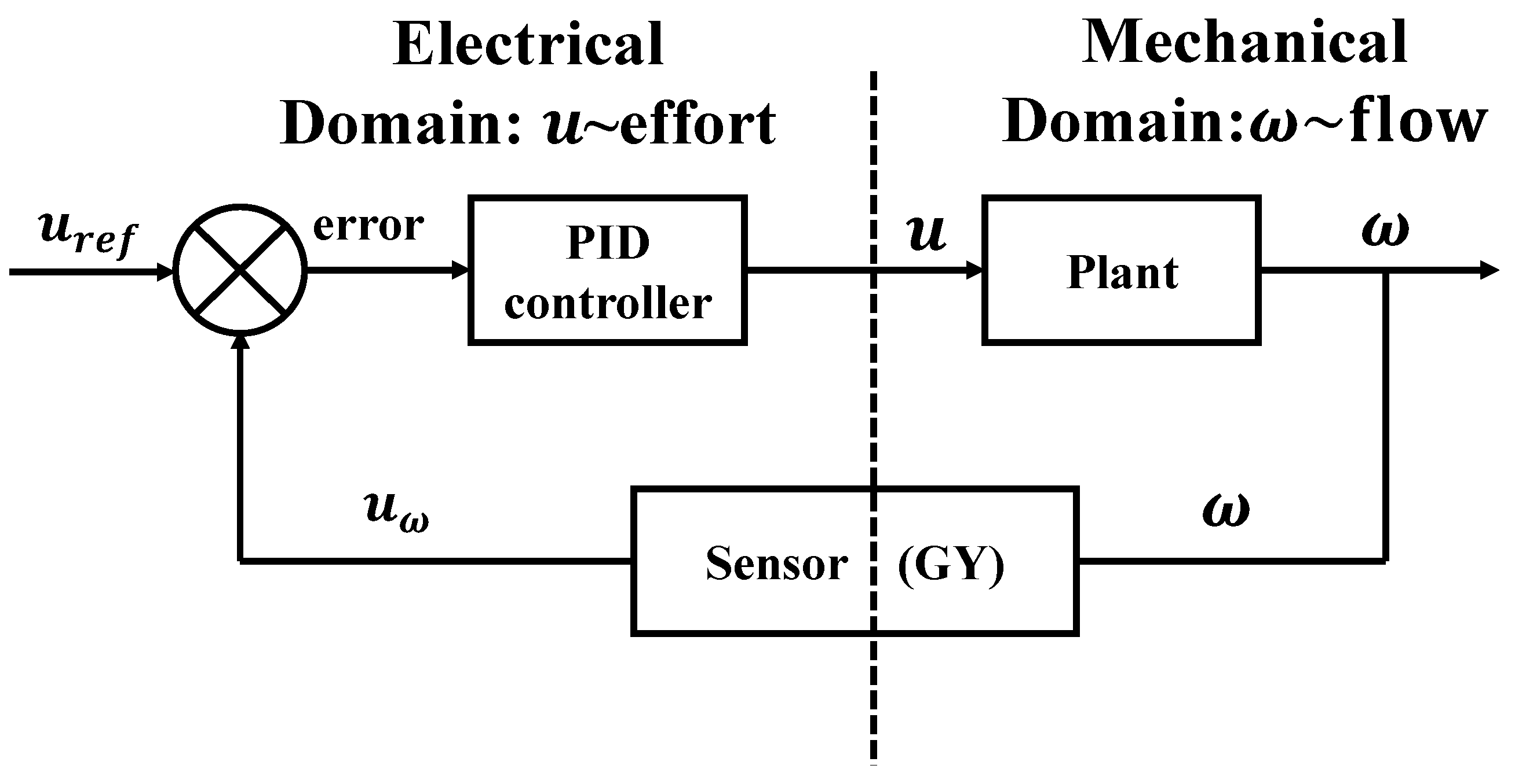
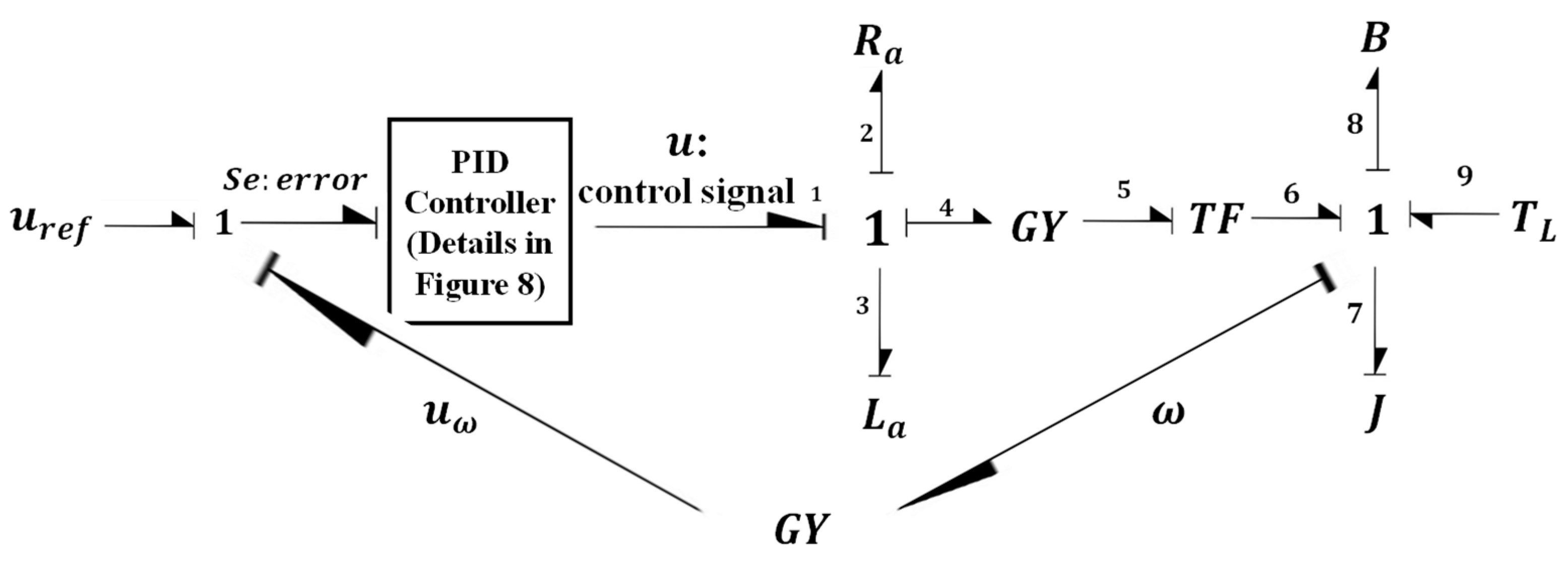
The bond graph of the PID controller is another main contribution of the paper. The input of the PID controller is the , which represents the error between the reference input value and the measurement output value. is the control signal of the DC motor plant. The bond graph of the DC motor speed control using the PID controller is shown in Figure 9. The GY symbol on the feedback bond graph is a tacho generator, which can convert the flow energy into effort energy.
Figure 8 and Figure 9 seem to be not simple enough for the electrical and control engineering students, but the figures could be a pleasant clear graphical language for the mechatronics students.
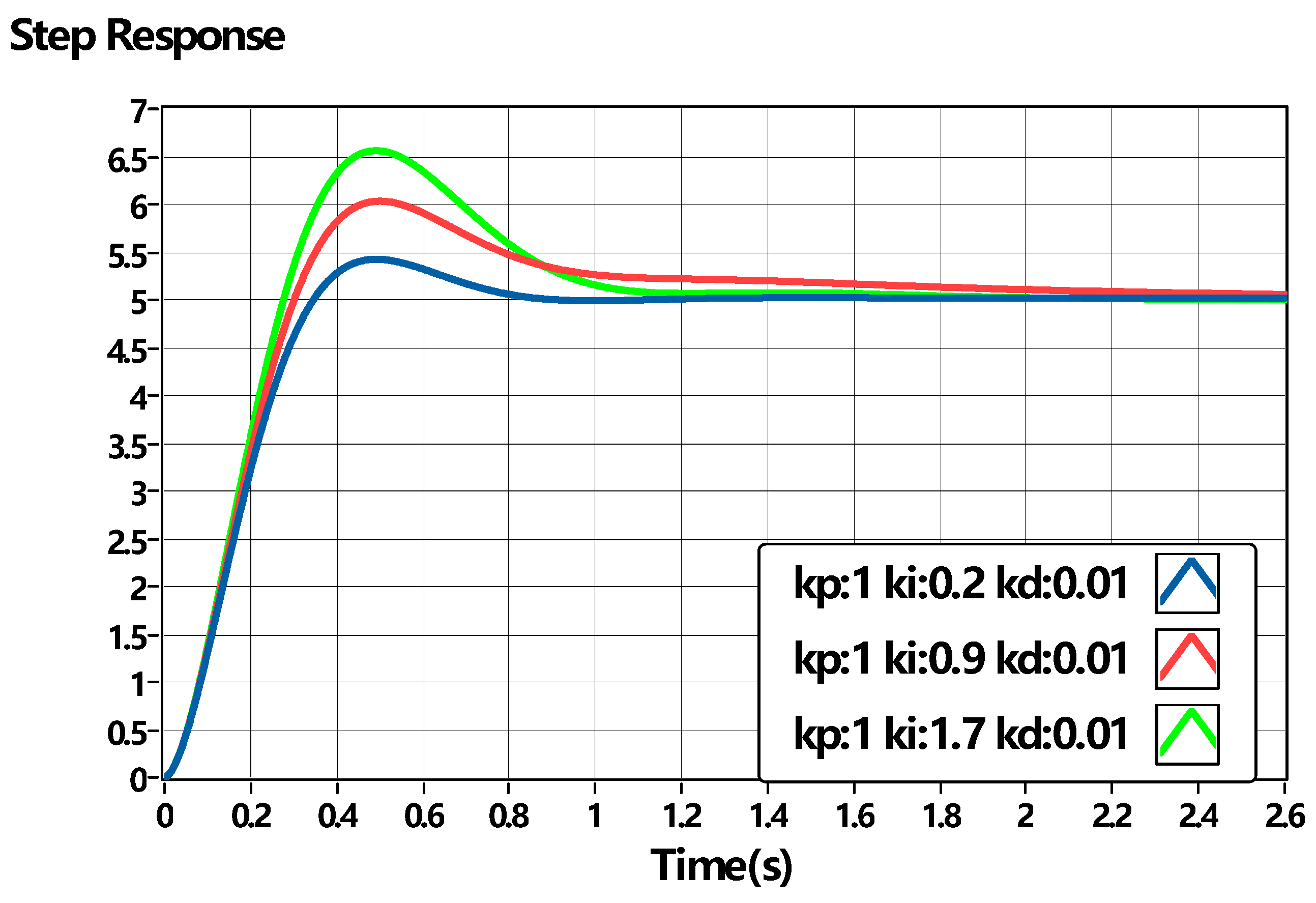
Figure 10 shows the step response of DC motor speed control using the PID controller with different . The overshoot of step response increases with the increases in the , Where . The results of the two methods are the same.
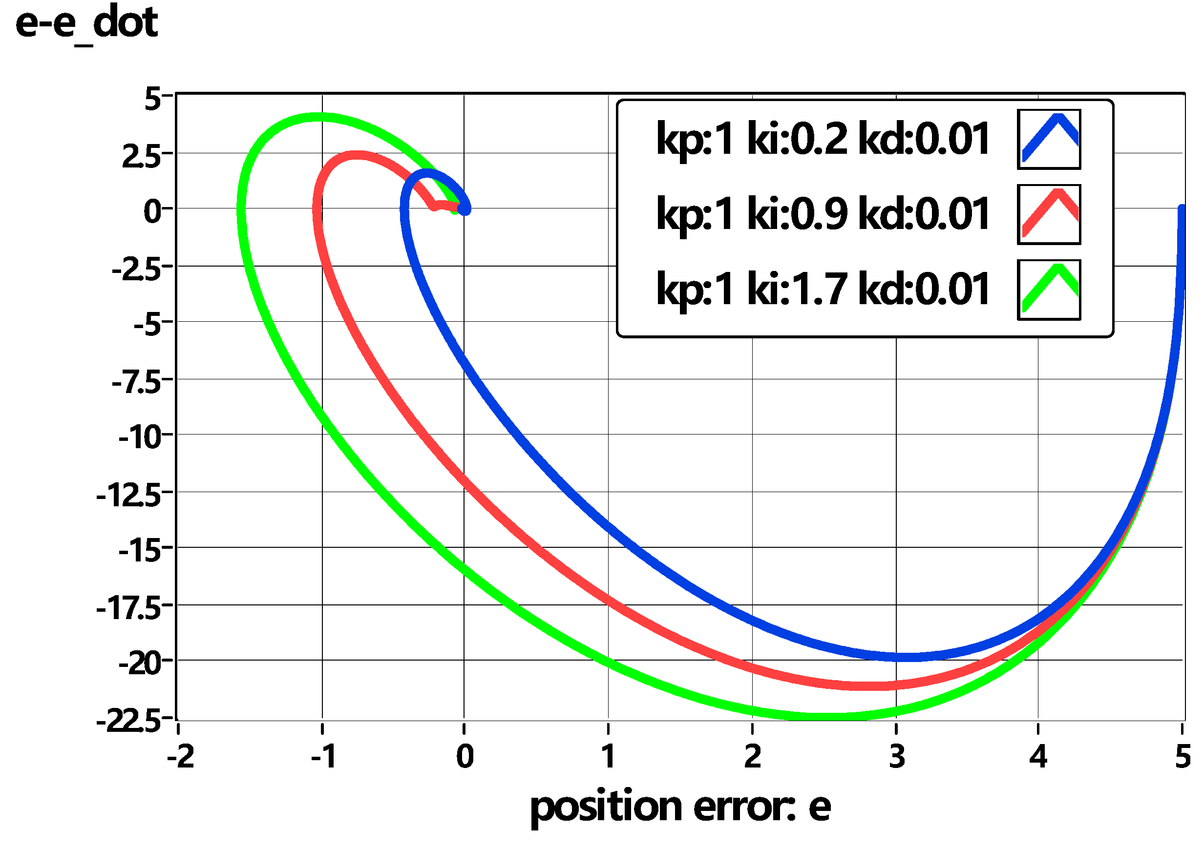
The plots can help students understand how the controller parameters affect the simulation results. Trajectories of the PID controller could express the characteristics of convergent performance. represent the position error and velocity error, respectively, in Figure 11. All the trajectories converge to the origin point in a finite time. The position error increases with the increase in .
The plots of the simulation from both methods are the same, but the methods to obtain the simulation result are different. The bond graph method could be considered a novel and powerful tool to solve simulation problems in mechatronics engineering.
4. Nonlinear Control with the Bond Graph Method for Undergraduate Students
Nonlinear control was introduced to the master students at first in the mechatronics engineering faculty at the University of Debrecen. With the iterative update of knowledge, the acceptance of nonlinear control for undergraduate students has increased. The nonlinear control is reintroduced in the undergraduate teaching materials because the sliding mode is complex enough in the theoretical part and simple enough for undergraduate students to implement. The sliding mode controller is one of the most efficient nonlinear controllers, which would apply to the BSc teaching curriculum. This section presents a normal sliding mode controller for position and speed tracking. Then, an adapt robust sliding mode controller method is introduced using the general model and real DC electrical machine parameters, respectively.
4.1. A Very Simple Sliding Mode Controller for Education Aim
The equations of the DC motor, and (), can be written in the following simple second-order form:
where is the moment of inertia; is the control input, i.e., the voltage of the motor; and is the disturbance, which must be a limited function. It can include external functions like the load torque and the internal first-order terms because of and . This means that, in this case, we do not need to know all the parameters of the motor, only is known exactly. We would like to emphasize to the students that during the design of the controller, the inductance of the rotor circuit (the electric time constant) is ignored. We consider it as unmodelled dynamics, which is covered by the controller. It is quite common in the engineering field that we start with a simple model. The goal is to use the simplest model, which provides satisfactory results.
The sliding surface is designed as follows:
where is satisfied Hurwitz condition, . Tracking error and tracking error derivative are shown as follows:
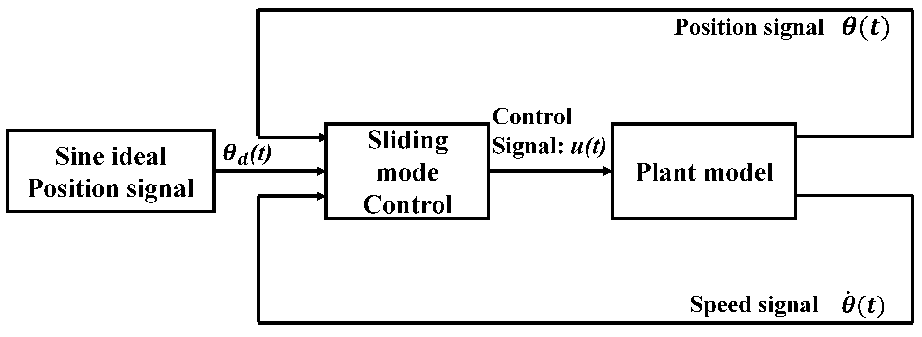
where, is the ideal angle signal. A general sliding mode control block diagram shows in Figure 12.
Our goal is that . The sliding mode occurs if . In sliding mode, the error tends to zero exponentially. The solution is quite easy from the mathematical point of view; we have to find a proper Lyapunov and use the Lyapunov condition. We will show this method in the next subsection but in our case, it can be explained by very elementary mathematical tools as well. If , then must be decreased, i.e., . If than must be increased, i.e., . The students can understand it. In other words, the signs of and must be opposite, so we ask the students to express and substitute and in the resulting formula. We can change the control signal only. That is why we use a term in the control signal which changes according to the sign of The easiest solution is the signum function. Finally, they can express the control signal . We can ignore all unknown terms of it and we assume that is big enough to determine the sign of . Since the operation area of a real motor is limited, the is limited as well.
In a certain area of , a very simple control law can be applied:
where the choice of must meet two contradictory conditions. If is too small, it cannot compensate for the disturbance; if it is too large, the chattering phenomenon causes problems. Therefore, it is advisable to calculate the so-called equivalent control signal , which ideally keeps the system in sliding mode.
The sign function has to compensate for our calculation error only. If the system is in sliding mode, then and , the equivalent control can be calculated from the latter.
Since is not known, it can be substituted by the signum function and the control signal designed as
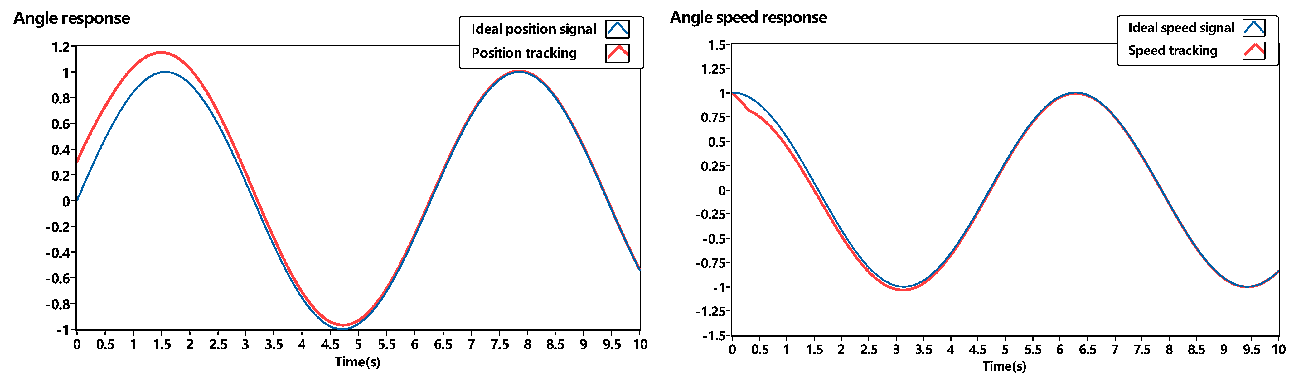
In this case, a smaller can be selected and the chattering can be reduced. The moment of inertia , , position target, and speed target initial condition are set to 0.3 and 1.0, respectively. , . The result simulation of position and speed tracking is shown in Figure 13.
The position and speed tracking performance is shown above. Some conclusions can be derived from the plots, the initial condition of the position affects the tracking performance in the general sliding mode controller. The speed tracking does not perform well even if the initial speed is the same as the ideal signal. An adaptive robust sliding mode controller is introduced to overcome the tracking error problem in the following section.
4.2. An Adaptive Robust Sliding Mode Controller
Adaptive control is a control method that can modify its characteristics to adapt to the changes in the dynamic characteristics of the target and disturbances. Robust control means that the control system maintains certain performance characteristics under certain parameter perturbations. By applying the adaptive robust sliding mode control, the position and speed tracking could track the ideal target well [33].
In the previous section, we emphasized that is exactly known. Now, we also allow parameter uncertainty in the case of inertia. Since this parameter uncertainty is also limited, it can also be included in the disturbance signal . In this section, as a didactic innovation, we present a method where the uncertainty of the parameter is not considered part of , but is calculated separately in such a way that the sliding mode control is combined with the estimation of a parameter. Parameter estimation itself is part of the curriculum.
The real and estimated inertia are and . The estimation error is
Our goal of is extended by an additional goal .
The Lyapunov function consists of two terms one for and one for .
where and . can be zero only if and , but these are our goals. If , then must be negative. Let us calculate ,
According to (),
Substituting and into Equation ,
The equivalent control signal is calculated from the first term of Since is inertia, then . This means, as a multiplier, does not change the sign of the product. It is not known, so it can be substituted by its estimation, . Two terms ( and ) are added to the equivalent control signal since in addition to suppressing the disturbance, parameter adaptation must also be ensured. If is big, then is dominant; if is small, then is dominant. The control signal designed in the following way can ensure convergence to the sliding mode:
where . Besides the control, a proper adaptation method must be selected as well. Substituting ) into ,
Equation can be derived as
Then, the adaptation law is selected by the last term of , which must be zero. Then, the adaptive law can be set as
4.3. Analysis and Fine-Tuning of the Adaptation
When , , where . When , . When , . The convergence of the system depends on the .
In order to prevent the control input signal from being too large due to too large , it is necessary to design the adaptive law so that the change in is within the range of []. A mapping adaptive algorithm is shown as
When exceeds the maximum value, if there is a tendency to continue to increase, , then the value of remains unchanged, then ; when exceeds the minimum value, if there is a tendency to continue to decrease, , then the value of remains unchanged, .
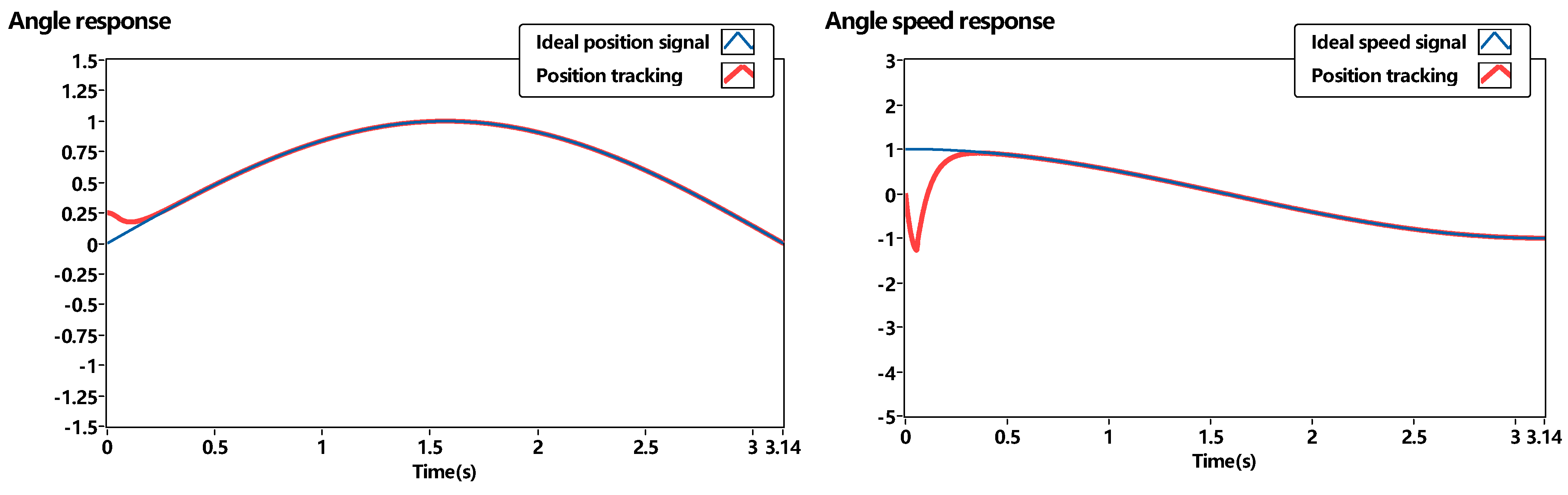
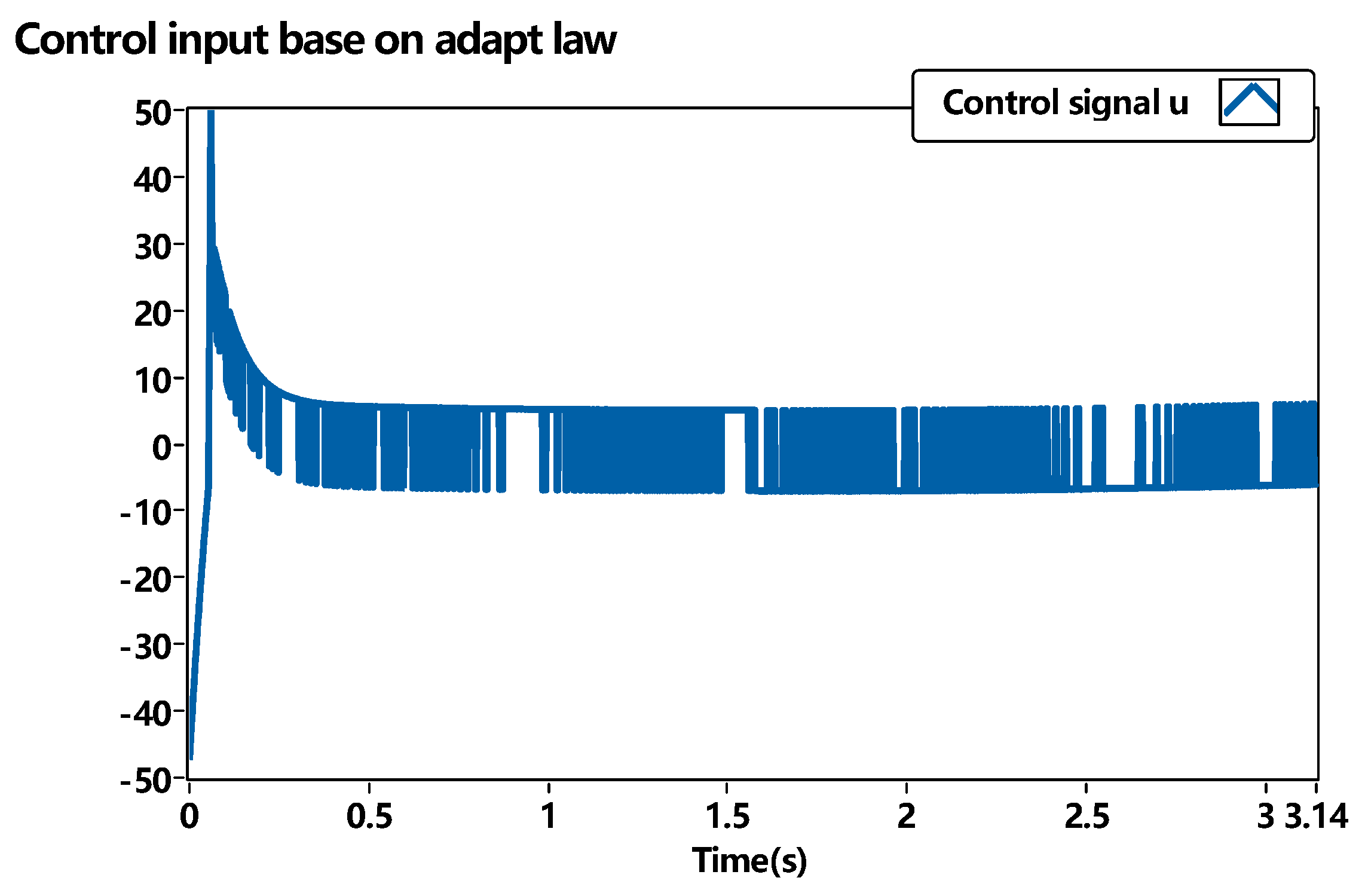
The position and speed tracking performance are shown in Figure 14. The initial condition of the position and speed are set to 0.25 and 0, respectively, where and target position signal is set to , , , , , and . . The control signal is designed as , where is the adaptive control part. Here, . is the sliding mode equivalent control. is the sliding control unit. The control signal can be limited by the adaptive law in Figure 15.
4.4. Adaptive Sliding Mode Controller Using Real DC Motor Parameters
After applying the simple sliding mode control and adaptive sliding mode control to the basic target model, the real DC motor parameters from Table 1 are applied in the adaptive sliding mode control.
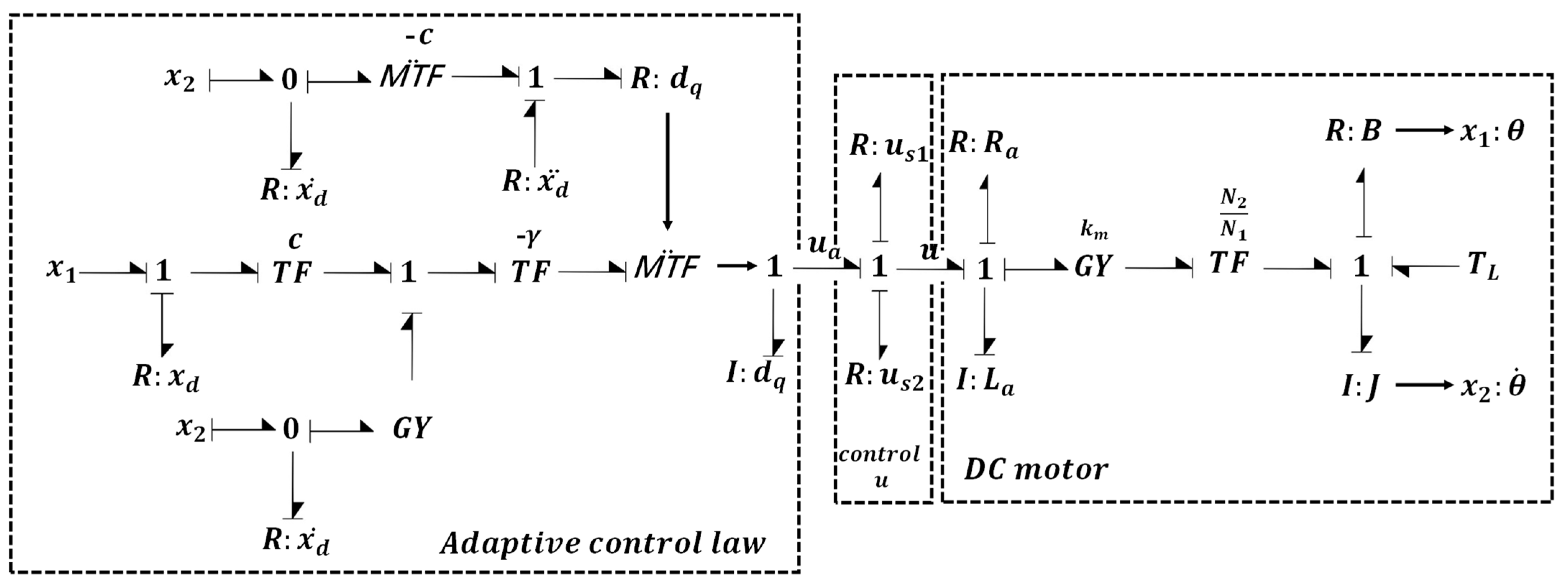
Another main contribution of this paper is to introduce the way to represent the sliding mode by using the bond graph method. The Bond graph of the adaptive sliding mode is shown in Figure 16. Compared with the mathematical equations, the bond graph method above presents all the energy flow of the adaptive robust sliding mode control. The elements and are the type of energy in the bond graph. is the modulated transformation; it can be considered as a gain in the bond graph. and are the position and speed, respectively, in the control loop. is the ideal position input.
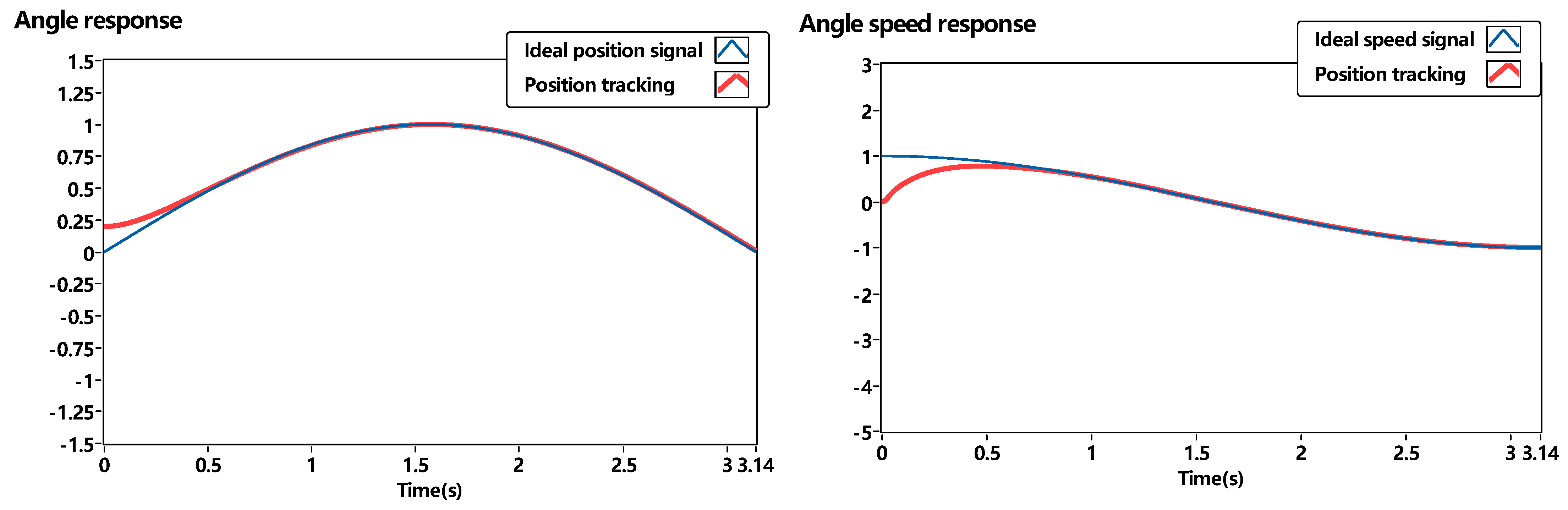
The position and speed tracking are shown in Figure 17; the position and speed initial condition is set to [0.2, 0.0]. The position performance can track the ideal position in a very short period, and the speed has no oscillation as the initial point differs from Figure 14.
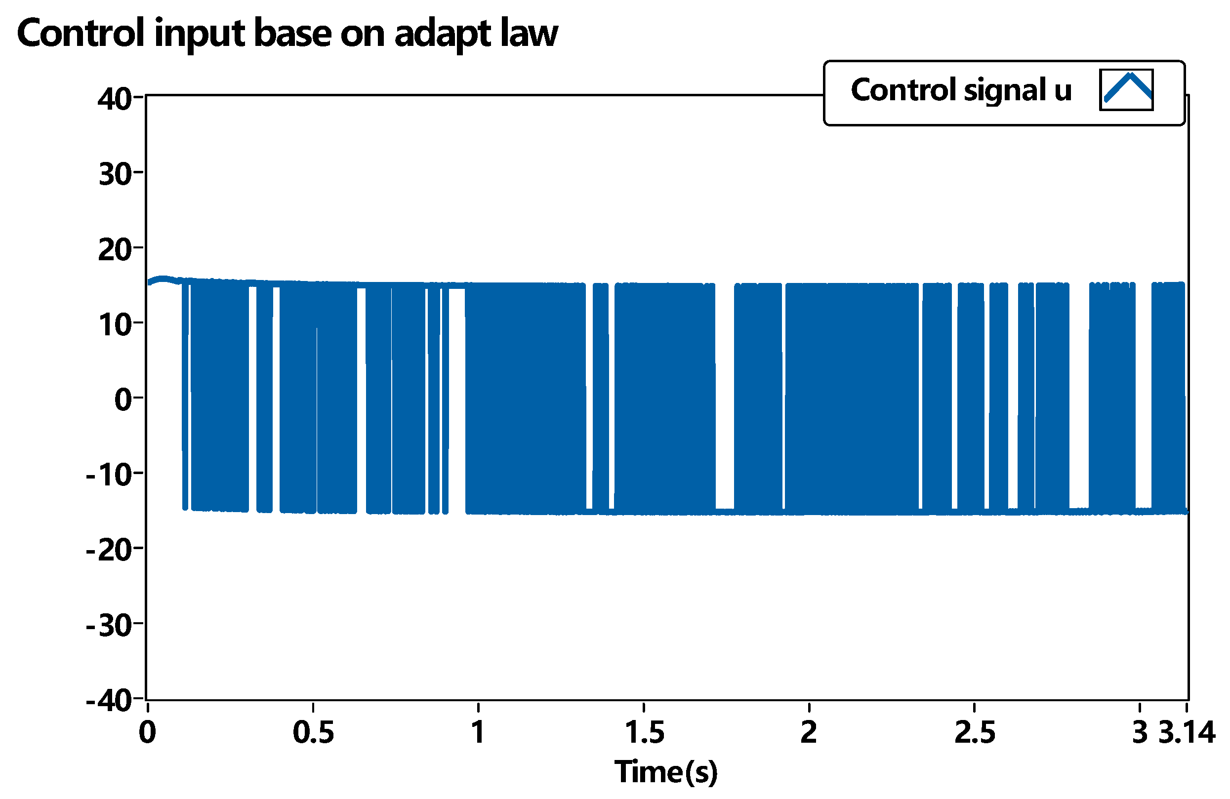
The control signal of the real DC motor parameters with saturation is shown in Figure 18. Compared with the control signal in Figure 15, the adaptive sliding mode controller is robust enough to track the position and speed with less oscillation and small amplification control signal input, where the reaching parameter , , , and sliding parameter . The plant model parameters are shown in Table 1.
In this section, a simple sliding mode with a general target is simulated in the first section. It presents an unsatisfied position and speed-tracking performance. Then, an adaptive robust sliding mode controller is proposed in the second subsection; it shows a better position and speed tracking performance. For the mechatronics engineering students, the bond graph of the whole system is presented in the third subsection; the bond graph demonstrates the synergy of the mechatronics system from a combination of multiple domains using the same graphical language.
The mathematical method (ODE) could help students build knowledge from the background perspective. And the bond graph method could help the researchers solve the problems from a novel graphical standpoint.
5. Test Results of the Modeling and Simulation Course
The final test from the ‘Modeling and Simulation’ course is evidence that using the bond graph method is easier than using the traditional mathematical technique to solve the mechatronics system.
Each year, the sample test is divided into three problems, with students solving each question using both the traditional mathematical approach and the bond graph method. And each answer would have two different outcomes. A claim is that the high-score strategy is the most convenient option for students to study for these three-year sample examinations.
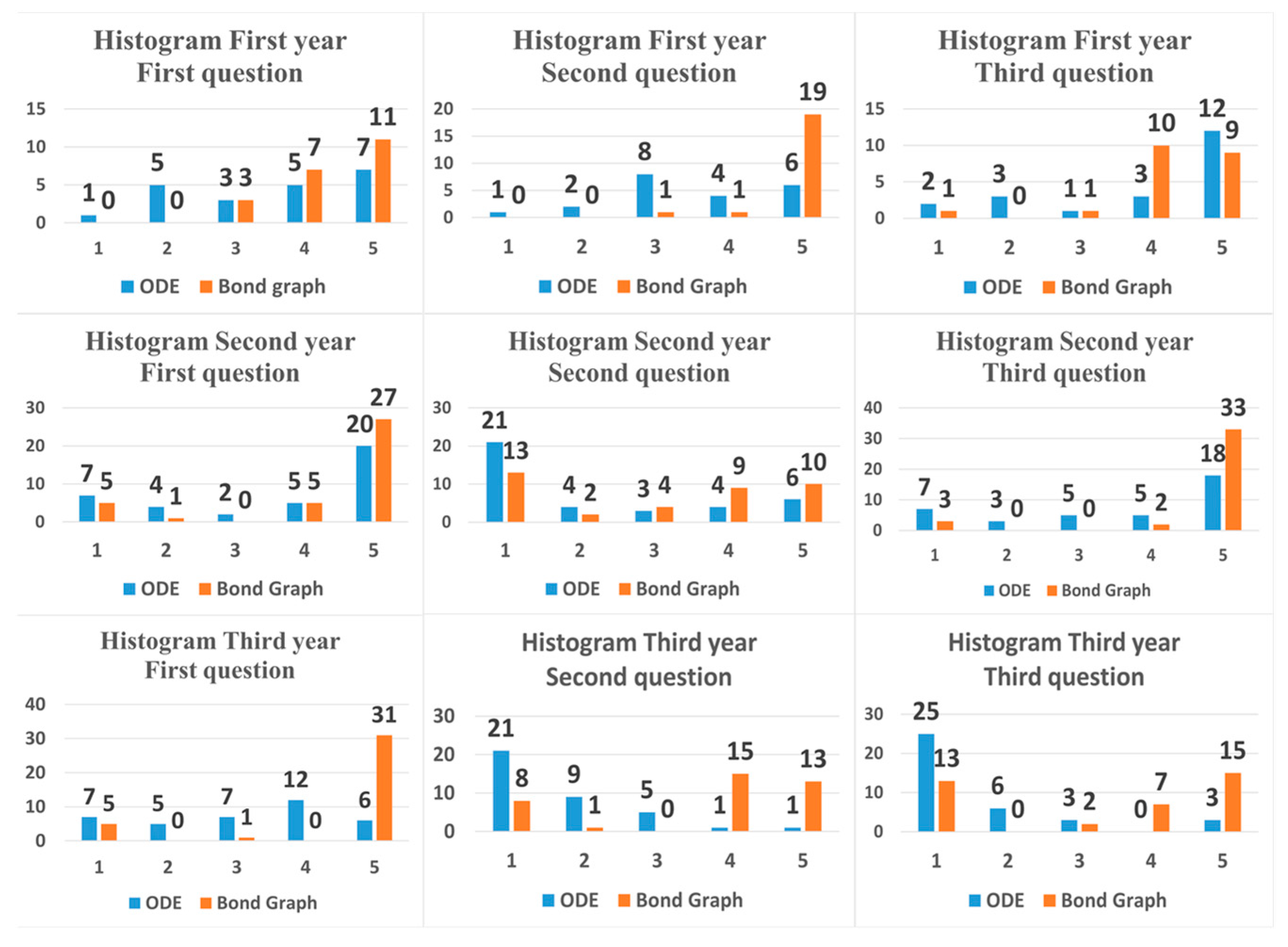
A total of 21 students were in the ‘Modeling and Simulation’ class in the first year; the test results were collected to compare the ODE method and the bond graph method. The questions were graded between 1 (fail) and 5 (excellent). The average and the mean of each question are shown in Table 3. According to the numerical connection, the average of the bond graph from questions one to three has increased by 16%, 26%, and 6%, respectively, when compared to the control group ODE average.
A total of 38 students attended the second-year test; the result is illustrated in Table 4. When compared to the control group ODE average, the average of the bond graph from questions one to three has grown by 22%, 16%, and 20%, respectively, according to the numerical connection.
In the third year, 37 students finished the exam shown the results in Table 5. According to the numerical connection, the average of the bond graph from questions one to three has increased by 25%, 39%, and 33%, respectively, as compared to the control group ODE average.
When comparing three years vertically, the sample of students has grown, and the disparity between the bond graph and the ODE has grown steadily each year. On the other hand, the bond graph has an advantage in the teaching of mechatronics. It also demonstrates that, for students, this is a more appropriate technique for studying mechatronics.
A t–test is performed to help determine whether there is a significant difference between the bond graph solution and the ODE solution. The null hypothesis is that the bond graph and the ODE have the same level of acceptance by students, which is reflected by the same students using different methods for the same problems.
where is the mean of the bond graph sample, is the standard deviation of the bond graph, and is the sample size of the bond graph. is the mean of the ODE sample, is the standard deviation of the ODE, and is the sample size of the ODE.
The t–test results are shown in Table 6:
In general, the significance level is chosen to be 0.05, and the value in Table 6 above shows that the bond graph solution and the ODE solution have a significant difference. It proves the bond graph method is more acceptable for mechatronics undergraduate students.
The three-year comparison histogram in Figure 19 shows that the students received a higher score when they used the bond graph to solve the problems compared with the ODE. Compared with the ODE, the bond graph is a more acceptable method for students to solve questions in mechatronics engineering. It is straightforward to conclude that the bond graph method is simpler than the traditional mathematical method in the ‘Modeling and Simulation’ subject. It does not mean that the bond graph will replace the ODE method in daily teaching, but the bond graph provides a new graphical perspective of the whole system. It makes the bond graph a practical tool for learning “modeling and simulation” subjects in mechatronics engineering and a smart tool for teachers to use.
6. Conclusions
There are three related subjects in the undergraduate student curriculum, “Basics of Mechatronics” (first semester), “Modelling and Simulation” (fifth semester), and “Control Theory”(sixth semester) in the Mechatronics Engineering Department, University of Debrecen. In this paper, the bond graph is presented as a novel and reliable tool in the “modeling and simulation” subject to connect these three related subjects. The subject synergy is connected by the bond graph method; it provides an efficient process to derive the simulation block diagram compared with the traditional mathematical method. On the one hand, the traditional method (ODE) helps students build the mathematical background; in the meantime, a blueprint of the whole system is presented graphically by using the bond graph method. On the other hand, multiple fields are represented using the same graphical language. It is also the objective and goal of scientific research to encompass a variety of research objects under the same theory. It is referred to as the synergy of mechatronics engineering. Another main contribution of the paper is the representation of the PID and sliding mode controller using the bond graph.
The example materials present that the bond graph method could provide a better view of the whole system from a graphical language, and it is a handy tool to solve the modeling questions for mechatronics students. The paper aims to provide mechatronics students with a step-by-step introduction to the state of the art in the field of the ‘modeling and simulation’ subject. Some dispersed problem assignments in Section Three and Section Four could properly guide students while also expanding their expertise. This novel teaching style may aid students in learning how to construct a simulation based on a real-world question.
Author Contributions
Conceptualization, Z.G.; methodology, Z.G.; software, P.T.S.; writing—original draft preparation, Z.G.; writing—review and editing, Z.G.; supervision, P.T.S. and P.K.; project administration, P.K. All authors have read and agreed to the published version of the manuscript.
Funding
Hungarian Research Fund (OTKA K143595).
Data Availability Statement
Not applicable.
Acknowledgments
The authors are very grateful to all the reviewers and editors for their valuable time spent. The authors wish to thank the support of the Hungarian Research Fund (OTKA K143595).
Conflicts of Interest
The authors declare no conflict of interest.
References
- Das, S. Mechatronic Modeling and Simulation Using Bond Graphs; CRC Press: Boca Raton, FL, USA, 2009; pp. 1–2. [Google Scholar]
- Karnopp, D.C.; Margolis, D.L.; Rosenberg, R.C. System Dynamics: Modeling, Simulation, and Control of Mechatronic Systems; John Wiley & Sons: Hoboken, NJ, USA, 2012. [Google Scholar]
- Isermann, R. On the design and control of mechatronic systems—A survey. IEEE Trans. Ind. Electron. 1996, 43, 4–15. [Google Scholar] [CrossRef]
- Allen, R.G. Mechatronics engineering: A critical need for this interdisciplinary approach to engineering education. In Proceedings of the 2006 IJME—INTERTECH Conference, New York, NY, USA, 19–21 October 2006; p. 205-085. [Google Scholar]
- Acar, M.; Parkin, R.M. Engineering education for mechatronics. IEEE Trans. Ind. Electron. 1996, 43, 106–112. [Google Scholar] [CrossRef]
- Papa, M.F.; De Castro, M.V.; Becker, P.; Martinez, E.M.; Olsina, L. Evaluation of Student’s Performance on a T-Shaped Degree. IEEE Trans. Educ. 2021, 64, 327–336. [Google Scholar] [CrossRef]
- MGarduño-Aparicio; Rodríguez-Reséndiz, J.; Macias-Bobadilla, G.; Thenozhi, S. A Multidisciplinary Industrial Robot Approach for Teaching Mechatronics-Related Courses. IEEE Trans. Educ. 2018, 61, 55–62. [Google Scholar] [CrossRef]
- Cellier, F.E. Bond graphs: The right choice for educating students in modeling continuous-time physical systems. Simulation 1995, 64, 154–159. [Google Scholar] [CrossRef]
- Ezzaki, M.; Fakhri, Y.; Ennima, S.; El Mortaji, H.; Jourani, M.; Abouchabaka, J. Bond Graph Model-Intelligent Online Diagnostics for Education. J. Theor. Appl. Inf. Technol. 2021, 99, 4425–4435. [Google Scholar]
- Roman, M.; Popescu, D.; Selişteanu, D. An interactive teaching system for bond graph modeling and simulation in bioengineering. J. Educ. Technol. Soc. 2013, 16, 17–31. [Google Scholar]
- Stankovski, S.; Tarjan, L.; Skrinjar, D.; Ostojic, G.; Senk, I. Using a Didactic Manipulator in Mechatronics and Industrial Engineering Courses. IEEE Trans. Educ. 2010, 53, 572–579. [Google Scholar] [CrossRef]
- López-Fernández, D.; Gordillo, A.; Alarcón, P.P.; Tovar, E. Comparing Traditional Teaching and Game-Based Learning Using Teacher-Authored Games on Computer Science Education. IEEE Trans. Educ. 2021, 64, 367–373. [Google Scholar] [CrossRef]
- Thoma, J.U. Introduction to Bond Graphs and Their Applications; Elsevier: Amsterdam, The Netherlands, 2016. [Google Scholar]
- Zanj, A.; He, F. A thermomechnical enhanced elastic model: Bond graph approach. In Proceedings of the 23rd International Congress on Sound and Vibration, Athens, Greece, 10–14 July 2016. [Google Scholar]
- Padilla Garcia, A.; Gonzalez-Avalos, G.; Ayala-Jaimes, G.; Barrera Gallegos, N.; Mendez-B, J.; Alvarado-Zamora, D. Tracking Control of Physical Systems with Application to a System with a DC Motor: A Bond Graph Approach. Symmetry 2022, 14, 755. [Google Scholar] [CrossRef]
- Djeziri, M.A.; Merzouki, R.; Bouamama, B.O.; Dauphin-Tanguy, G. Robust fault diagnosis by using bond graph approach. IEEE/ASME Trans. Mechatron. 2007, 12, 599–611. [Google Scholar] [CrossRef]
- Cooper, J.L.; Alibali, M.W. Visual Representations in Mathematics Problem-Solving: Effects of Diagrams and Illustrations; North American Chapter of the International Group for the Psychology of Mathematics Education: Kalamazoo, MI, USA, 2012.
- Ruf, V.; Horrer, A.; Berndt, M.; Hofer, S.I.; Fischer, F.; Fischer, M.R.; Zottmann, J.M.; Kuhn, J.; Küchemann, S. A Literature Review Comparing Experts’ and Non-Experts’ Visual Processing of Graphs during Problem-Solving and Learning. Educ. Sci. 2023, 13, 216. [Google Scholar] [CrossRef]
- Boaler, J.; Chen, L.; Williams, C.; Cordero, M. Seeing as understanding: The importance of visual mathematics for our brain and learning. J. Appl. Comput. Math. 2016, 5, 325. [Google Scholar] [CrossRef]
- Zenan, G.; Szemes, P.T.; Korondi, P. October. Bond graph-based teaching method to enhance the synergy of mechatronics in Lab VIEW. In Proceedings of the 2022 IEEE 9th International Conference on e-Learning in Industrial Electronics (ICELIE), Brussel, Belgium, 17–20 October 2022; IEEE: Piscataway, NJ, USA; pp. 1–6. [Google Scholar] [CrossRef]
- Suman, S.K.; Giri, V.K. March. Speed control of DC motor using optimization techniques based PID Controller. In Proceedings of the 2016 IEEE International Conference on Engineering and Technology (ICETECH), Coimbatore, India, 17–18 March 2016; pp. 581–587. [Google Scholar] [CrossRef]
- Abdulameer, A.; Sulaiman, M.; Aras, M.S.M.; Saleem, D. Tuning methods of PID controller for DC motor speed control. Indones. J. Electr. Eng. Comput. Sci. 2016, 3, 343–349. [Google Scholar] [CrossRef]
- Sahputro, S.D.; Fadilah, F.; Wicaksono, N.A.; Yusivar, F. Design and implementation of adaptive pid controller for speed control of DC motor. In Proceedings of the 2017 15th International Conference on Quality in Research (QIR): International Symposium on Electrical and Computer Engineering, Nusa Dua, Bali, Indonesia, 24–27 July 2017. [Google Scholar] [CrossRef]
- Kamdar, S.; Brahmbhatt, H.; Patel, T.; Thakker, M. Sensorless speed control of high speed brushed dc motor by model identification and validation. In Proceedings of the 2015 5th Nirma University International Conference on Engineering (NUICONE), Ahmedabad, India, 26–28 November 2015; pp. 1–6. [Google Scholar] [CrossRef]
- Utkin, V.; Guldner, J.; Shijun, M. Sliding Mode Control in Electromechanical Systems; CRC Press: Boca Raton, FL, USA, 1999; Volume 34. [Google Scholar]
- Dursun, E.H.; Durdu, A. Speed control of a DC motor with variable load using sliding mode control. Int. J. Comput. Electr. Eng. 2016, 8, 219–226. [Google Scholar] [CrossRef]
- Maghfiroh, H.; Sujono, A.; Apribowo, C.H.B. Basic tutorial on sliding mode control in speed control of DC-motor. J. Electr. Electron. Inf. Commun. Technol. 2020, 2, 1–4. [Google Scholar] [CrossRef]
- Fink, N.; Zenan, G.; Szemes, P.; Korondi, P. Comparison of Direct and Inverse Model-based Disturbance Observer for a Servo Drive System. Acta Polytech. Hung. 2023, 20, 205–228. [Google Scholar] [CrossRef]
- Ji, P.; Li, C.; Ma, F. Sliding Mode Control of Manipulator Based on Improved Reaching Law and Sliding Surface. Mathematics 2022, 10, 1935. [Google Scholar] [CrossRef]
- Filippov, A.G. Application of the Theory of Differential Equations with Discontinuous Right-hand Sides to Non-linear Problems in Automatic Control. IFAC Proc. Vol. 1960, 1, 923–925. [Google Scholar] [CrossRef]
- Borutzky, W. Bond Graph Methodology: Development and Analysis of Multidisciplinary Dynamic System Models; Springer Science & Business Media: Berlin/Heidelberg, Germany, 2009. [Google Scholar] [CrossRef]
- Dorf, R.C.; Bishop, R.H. Modern Control Systems, 12th ed.; Prentice Hall: Upper Saddle River, NJ, USA, 2011; pp. 51–52. [Google Scholar]
- Liu, J. Sliding mode control design and MATLAB simulation. In The Basic Theory and Design Method; Tsinghua University Press: Beijing, China, 2012; pp. 35–37. [Google Scholar]
Figure 1.
Abstraction and non-linear features of mechatronics subjects.

Figure 2.
Schematic of DC electrical machine with a gearbox and a load.

Figure 3.
Bond graph of the DC motor.

Figure 4.
Block diagram derived from bond graph method.

Figure 5.
The block diagram in LabVIEW.

Figure 6.
Comparison of two methods.

Figure 7.
Block diagram of the control system.

Figure 8.
Bond graph of PID controller.

Figure 9.
Bond graph of the whole system.

Figure 10.
DC motor speed control using PID controller with varying .

Figure 11.
PID controller with vary .

Figure 12.
A general sliding mode control.

Figure 13.
A general sliding mode control position and speed tracking.

Figure 14.
Position and speed tracking of adaptive sliding mode controller.

Figure 15.
Control signal of the adaptive sliding mode controller.

Figure 16.
Bond graph of DC motor position and speed tracking using adaptive sliding mode.

Figure 17.
Position and speed tracking of adaptive robust SMC.

Figure 18.
Control of adaptive robust sliding mode control using real parameters.

Figure 19.
Histogram of the three questions results over three years.


Table 1.
Parameters of Maxon A-max 26 (110961).
| Maxon A-Max 26 (110961) | |
|---|---|
| Nominal torque | 17.4 mNm |
| Nominal current | 1.08 A |
| Terminal resistance | 3.13 Ω |
| Terminal inductance | 0.333 mH |
| Mechanical time constant | 14.7 ms |
| Rotor inertia | |
| Torque constant | 16.8 mNm/A |
Table 2.
Parameters of Gear Drive (110396).
| Gear Drive (110396) | |
|---|---|
| Reduction | 81:1 |
| Number of stages | 3 |
| Max continuous Torgue at Gear output | 1.8Nm |
| Max efficiency | 80% |
Table 3.
The first-year test result.
| Question 1 | Question 2 | Question 3 | |
|---|---|---|---|
| ODE average | 3.57 | 3.57 | 3.95 |
| Bond graph average | 4.38 | 4.86 | 4.24 |
| ODE mean | 3.28 | 3.35 | 3.56 |
| Bond graph mean | 4.31 | 4.83 | 4.06 |
| Average (bond graph-OED) difference | 0.81 | 1.29 | 0.29 |
| Mean (bond graph-ODE) difference | 1.03 | 1.48 | 0.51 |
| Average (bond graph-ODE) difference (%) | 16% | 26% | 6% |
| Mean (bond graph-ODE) difference (%) | 21% | 30% | 10% |
Table 4.
The second-year test result.
| Question 1 | Question 2 | Question 3 | |
|---|---|---|---|
| ODE average | 3.17 | 2.21 | 3.65 |
| Bond graph average | 4.26 | 3.03 | 4.63 |
| ODE mean | 3.19 | 1.72 | 3.14 |
| Bond graph mean | 3.84 | 2.47 | 4.35 |
| Average (bond graph-OED) difference | 1.09 | 0.82 | 1.00 |
| Mean (bond graph-ODE) difference | 0.64 | 0.72 | 1.21 |
| Average (bond graph-ODE) difference (%) | 22% | 16% | 20% |
| Mean (bond graph-ODE) difference (%) | 13% | 14% | 24% |
Table 5.
The third-year test result.
| Question 1 | Question 2 | Question 3 | |
|---|---|---|---|
| ODE average | 3.14 | 1.70 | 1.65 |
| Bond graph average | 4.41 | 3.65 | 3.30 |
| ODE mean | 2.75 | 1.49 | 1.39 |
| Bond graph mean | 3.97 | 3.15 | 2.65 |
| Average (bond graph-OED) difference | 1.27 | 1.95 | 1.65 |
| Mean (bond graph-ODE) difference | 1.27 | 1.66 | 1.26 |
| Average (bond graph-ODE) difference (%) | 25% | 39% | 33% |
| Mean (bond graph-ODE) difference (%) | 24% | 33% | 25% |
Table 6.
value of three questions among three years.
| Question 1 | Question 2 | Question 3 | |
|---|---|---|---|
| First year | 0.00930 | 0.00001 | 0.26690 |
| Second year | 0.00266 | 0.00008 | 0.00004 |
| Third year | 0.0000004 | 0.00000058 | 0.0000025 |
Disclaimer/Publisher’s Note: The statements, opinions and data contained in all publications are solely those of the individual author(s) and contributor(s) and not of MDPI and/or the editor(s). MDPI and/or the editor(s) disclaim responsibility for any injury to people or property resulting from any ideas, methods, instructions or products referred to in the content. |
© 2023 by the authors. Licensee MDPI, Basel, Switzerland. This article is an open access article distributed under the terms and conditions of the Creative Commons Attribution (CC BY) license (https://creativecommons.org/licenses/by/4.0/).
Share and Cite
MDPI and ACS Style
Guo, Z.; Korondi, P.; Szemes, P.T. Bond-Graph-Based Approach to Teach PID and Sliding Mode Control in Mechatronics. Machines 2023, 11, 959. https://doi.org/10.3390/machines11100959
AMA Style
Guo Z, Korondi P, Szemes PT. Bond-Graph-Based Approach to Teach PID and Sliding Mode Control in Mechatronics. Machines. 2023; 11(10):959. https://doi.org/10.3390/machines11100959
Chicago/Turabian StyleGuo, Zenan, Péter Korondi, and Péter Tamás Szemes. 2023. "Bond-Graph-Based Approach to Teach PID and Sliding Mode Control in Mechatronics" Machines 11, no. 10: 959. https://doi.org/10.3390/machines11100959
Note that from the first issue of 2016, this journal uses article numbers instead of page numbers. See further details here.