Article

Selective Harmonic Elimination in a Cascaded Multilevel Inverter of Distributed Power Generators Using Water Cycle Algorithm

1
Department of Electrical Engineering, National University of Computer and Emerging Sciences, Lahore 54000, Pakistan
2
Department of Electrical Engineering, University of Engineering and Technology, Lahore 54000, Pakistan
3
ISEN Yncréa Ouest, L@bISEN, 29200 Brest, France
4
Institut de Recherche Dupuy de Lôme (UMR CNRS 6027 IRDL), University of Brest, 29238 Brest, France
5
Logistics Engineering College, Shanghai Maritime University, Shanghai 201306, China
*
Author to whom correspondence should be addressed.
Machines 2022, 10(5), 399; https://doi.org/10.3390/machines10050399
Submission received: 22 April 2022 / Revised: 16 May 2022 / Accepted: 16 May 2022 / Published: 20 May 2022
(This article belongs to the Section Electromechanical Energy Conversion Systems)

Abstract

:
This research paper proposes the application of a meta-heuristic algorithm, namely the water cycle algorithm (WCA), for optimizing the performance of a multi-level inverter for a distributed energy resources-based smart grid system. The aim is to find the optimal switching angles to achieve selective harmonic elimination. To exhibit the effectiveness of the proposed algorithm and evaluate the results, a three-phase seven-level cascaded multilevel inverter (CHBMLI) is used. This paper demonstrates the efficacy of the proposed algorithm by performing a rigorous comparison with existing meta-heuristic algorithms. Independent sample t-tests for different population sizes are demonstrated, which reflect the better performance of the proposed algorithm’s results. For the comparison, crucial parameters for optimization, including population size and number of iterations, are kept the same for the proposed WCA and other algorithms. Since we are solving a minimization problem, a lower fitness value is focused. In our research paper, we show how the proposed algorithm attains a lower fitness value and fast rate of convergence. For different values of the modulation index, WCA performs better than particle swarm optimization (PSO) and the firefly algorithm (FA). For a particular case of a modulation index value of 0.8, the minimum value found by WCA over 50 samples is 0.0001, whereas that of PSO and FA are 0.0223 and 0.0433, respectively, which shows that WCA has better accuracy. The results clearly present that the proposed algorithm provides a competitive percentage of elimination of selected harmonics when compared with other meta-heuristic algorithms.

1. Introduction

Over the last few decades, multilevel inverters have found many industrial applications. They are being employed in medium voltage and high power electrical drives [1]. Multilevel inverters have also been extensively utilized in flexible AC transmission (FACT) and high voltage direct transmission (HVDC) based systems [2,3]. Multilevel inverters have three types: flying capacitor, diode clamped and cascaded H-bridge multilevel inverters (CHBMLI) [4,5,6]. Modularity and repetitive structure makes CHBMLI extensively used in renewable energy systems (RES) [7,8,9]. Additionally, CHBMLI has a fewer number of components. The employment of separate DC sources is also its desirable feature, especially in PV systems [10,11]. Figure 1 presents an application of CHBMLI in a distributed energy resources-based power grid system. It consists of pre-defined H-bridge cells connected in series. Each cell has its independent DC power supply, and these power supplies can be the same or different. The number of levels obtained in a k-level CHBMLI is (2k + 1).
Nowadays, a major challenge with a multilevel inverter (MLI) is focused on improving the power quality. For CHBMLI control, several modulation techniques exist in the literature. Conventional pulse width modulation (PWM), sinusoidal PWM, and space vector modulation are high-frequency switching techniques with a transient response. Furthermore, different carrier-based PWM techniques and carrier-less PWM techniques are introduced that effectively reduce distortion and reduce the electromagnetic interference (EMI). Inverter efficiency can be improved by the employment of low-pass filters of a high-order, which suppress high-order harmonics. However, dominant low-order harmonics, namely the third, fifth and seventh harmonics, cannot be eliminated completely using PWM-based switching techniques.
Selective harmonic elimination (SHE) is a low switching frequency technique. In SHE, switching angles are determined that eliminate the specific lower order harmonics while maintaining a fundamental order harmonic. These switching angles are determined by solving SHE equations. Various constraints need to be taken care of while determining switching angles using SHE equations. These include restricting angles between 0 and π 2 (assuming quarter-wave symmetry) and maintaining the fundamental to a defined value. The challenge associated while eliminating harmonics using the SHE technique is the solution to solve complex non-linear equations, as they contain trigonometric terms and exhibit a multi-modal nature.
Various methods have been discussed in the literature to solve SHE transcendental equations, which include numerical, algebraic methods, and bio-inspired methods [12]. In particular, numerical methods have been discussed in the literature to solve SHE equations. In [13], the application of Walsh functions for solving SHE equations is discussed. To solve SHE equations, the homotopy algorithm is applied in [14]. Sequential programming and Newton–Raphson methods are also discussed to solve SHE equations in [15,16], respectively. Although numerical methods give accurate solutions, they have a tendency to get trapped in local optima due to dependency on initial guess.
Algebraic methods, such as the resultant theory method [17], theory of Groebner bases [18], Wu method [19], symmetric polynomial [20], and power sum methods [21], have also been discussed in the literature to solve SHE complex nonlinear equations. Algebraic methods work by transforming non-linear algebraic equations into polynomial equations, and they do not require an initial guess. Hence, they are better as compared to numerical methods due to the non-requirement of an initial guess. However, these methods are only suitable for low-level inverters. With the increase in the number of inverter levels, the complexity and computational burden of these methods also increase and they become unsuitable for real-time control of high-level power inverters.
In the past, many bio-inspired metaheuristic algorithms have been reported in the literature to solve SHE equations for CHBMLI. Early metaheuristic algorithms include the genetic algorithm (GA) and its variants [22]. GA is applied for the harmonic elimination of the 5th, 7th, and 11th harmonics in a three-phase nine-level inverter in [23], but the authors do not provide solutions for all values of the modulation index. Particle swarm optimization (PSO) is also applied to CHBMLI for SHE in [24]. In [25], the author presents the application of the bee algorithm (BA) to a 7-level inverter and compares its performance with GA. The author concludes that BA surpasses GA in the attainment of an accurate global minima, and the rate of convergence of BA is also better. In [26], the cuckoo search algorithm (CSA) is utilized for SHE in a 7-level CHBMLI. The author compares the performance of CSA with BA and GA and determines that CSA performs better than BA in eliminating selected harmonics, but the comparison in terms of convergence speed is not provided. The bat optimization algorithm (BOA) is applied to a three-phase 7-level CHBMLI for solving SHE equations [27], and the comparison of the reported algorithm is performed with GA and BA. The author reports the superiority of BOA over GA and BA in eliminating harmonics but does not compare the aforementioned techniques in terms of speed of convergence. In [28], employment of the firefly algorithm (FA) is reported for SHE in 11-level CHBMLI, having equal and unequal DC sources. The author suggests that FA performs better than PSO, GA, modified PSO, and NR, but a convergence comparison is not performed. Recently, many newly developed evolutionary algorithms have been applied for the SHE problem in CHBMLI [12]. The ant colony optimization (ACO) algorithm is applied to a three-phase 5-level inverter, and it is compared with GA in [29]. In [30], grey wolf optimizer (GWO) is reported for harmonic elimination in 11- and 15-level CHBMLIs, and its comparison is performed with PSO. It is reported that GWO outperforms PSO. In [31], the modified grey wolf optimizer (MGWO) is reported for the harmonic elimination problem in hybrid CHBMLI. In [32], a bacterial foraging algorithm is applied to solve SHE equations. The newly developed salt swarm algorithm (SSA) is also reported for the harmonic elimination problem in a 5-level inverter, and the author shows that SSA performs better than PSO in terms of convergence [33].
In the aforementioned papers, various algorithms have been applied to solve SHE equations for multilevel inverters. These algorithms require the tuning of multiple parameters for their optimal performance. This research proposes a state-of-the-art water cycle algorithm (WCA) for solving the SHE equations in a CHBMLI. WCA is simple to implement and requires the tuning of only one parameter for its optimal performance. The major contributions of this paper are as follows:
  • Application of water cycle algorithm for solving selective harmonic equations of a cascaded H-bridge multi-level inverter.
  • Comparison of computational complexity along with accuracy and speed of convergence with other meta-heuristic algorithms are provided to prove the effectiveness of the water cycle algorithm.
  • Statistical comparison between different meta-heuristic algorithms using the independent sample t-test is also provided.
The remaining paper is organized as follows: Section 2 explains the problem formulation for CHBMLI; Section 3 illustrates the water cycle algorithm; Section 4 explains the simulation setup; Section 5 presents the results and analysis; and finally, Section 6 concludes the findings of the proposed work.

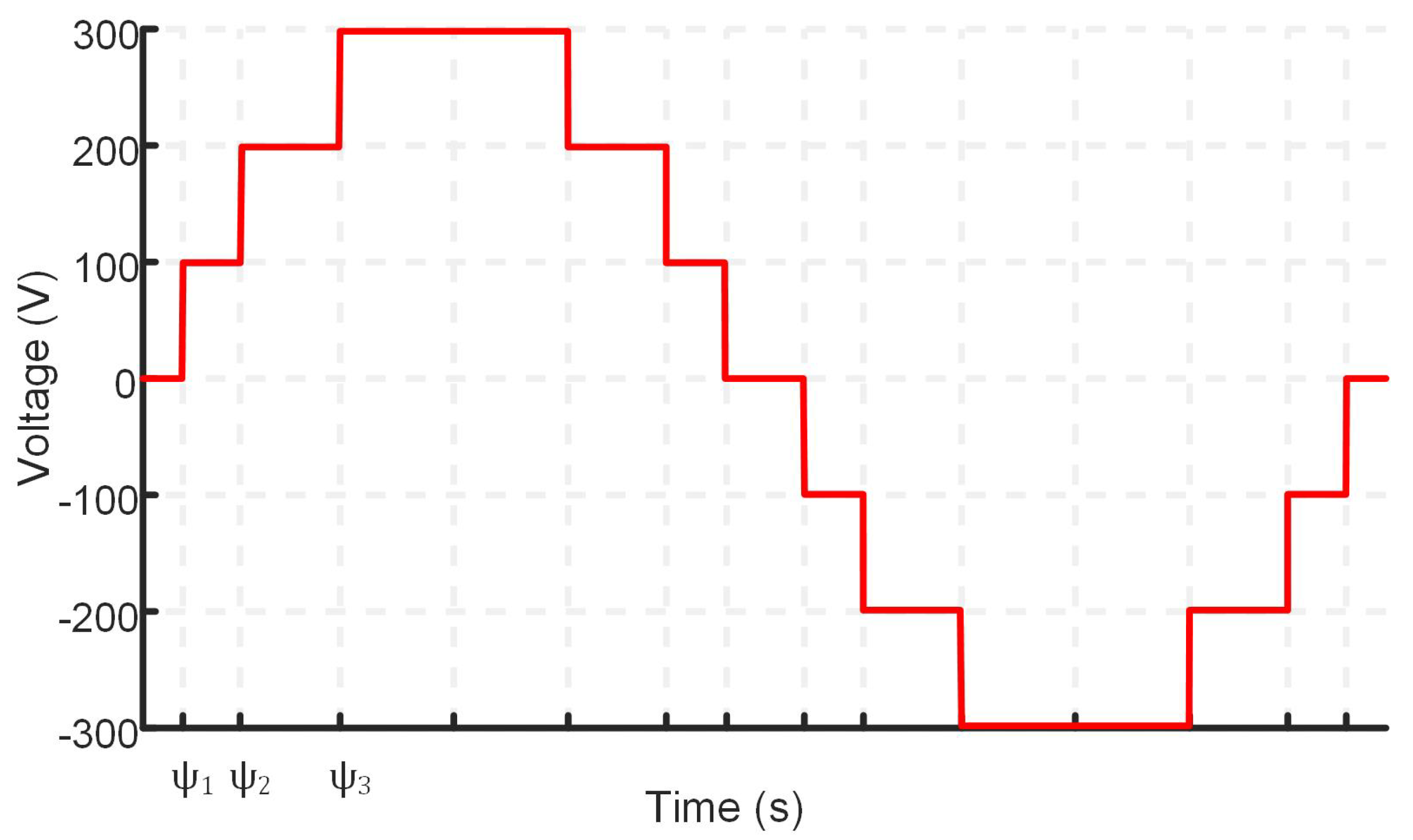
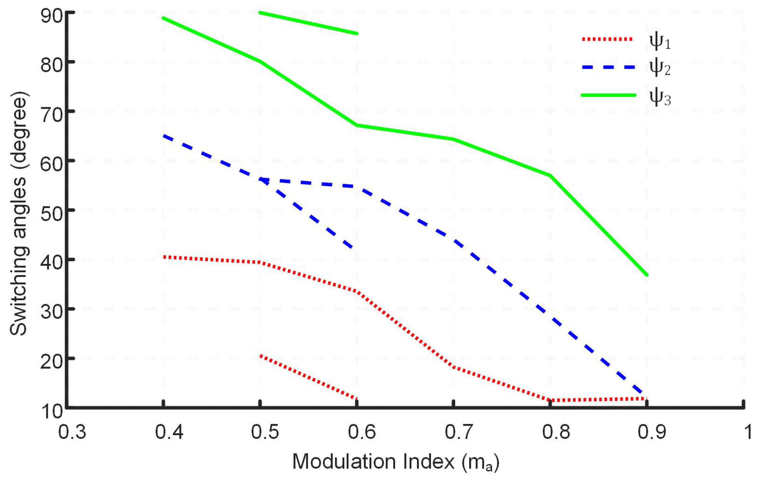
2. CHBMLI Problem Formulation

The SHE technique involves solving non-linear equations for CHBMLI. These equations are obtained by decomposing the waveform into its Fourier series. The even and cosine terms get zero due to the quarter wave symmetry due to the nature of the function being odd. Triplen harmonics also becomes canceled out in the line voltage.
For a M-Level three phase CHBMLI, having k cells, the degree of freedom is k, and k 1 harmonics can be eliminated. The transcendental equations expressing the fundamental and dominant low order non-triplen harmonics for a CHBMLI can be formulated as given in Equations (1) and (2).
V 1 = 4 V d c π ( c o s ( ψ 1 ) + c o s ( ψ 2 ) + c o s ( ψ 3 ) . . . . . . c o s ( ψ k ) )
0 = 4 V d c n π ( c o s ( n ψ 1 ) + c o s ( n ψ 2 ) + c o s ( n ψ 3 ) . . . . . . c o s ( n ψ k ) )
The fundamental component can be expressed in terms of the modulation index ( m a ) as given in Equation (3).
c o s ( ψ 1 ) + c o s ( ψ 2 ) + c o s ( ψ 3 ) . . . . . . c o s ( ψ k ) = k m a = m
where,
m = V 1 4 V d c π
m a = V 1 V m a x = V 1 4 k V d c π = m k
where V 1 is the fundamental value of the phase voltage obtained by the H-bridge. V m a x is the maximum value of the phase voltage obtained by CHBMLI, and k is the number of H-bridge cells. V m a x is obtained when all the switching angles are zero, i.e.,
V m a x = 4 k V d c π
For a 7-level CHBMLI, the stepped waveform is shown in Figure 2. Following the illustration and modeling, SHE equations for a 7-Level CHBMLI can be formulated as follows:
c o s ( ψ 1 ) + c o s ( ψ 2 ) + c o s ( ψ 3 ) = 3 m a
c o s ( 5 ψ 1 ) + c o s ( 5 ψ 2 ) + c o s ( 5 ψ 3 ) = 0
c o s ( 7 ψ 1 ) + c o s ( 7 ψ 2 ) + c o s ( 7 ψ 3 ) = 0
Taking the cosine terms in Equation (7) to the right hand side, we obtain
3 m a ( c o s ( ψ 1 ) + c o s ( ψ 2 ) + c o s ( ψ 3 ) ) = 0
Since we are eliminating specific harmonics while maintaining the fundamental component to a particular value, we define an objective function which relates all the harmonics and the fundamental component. Taking this into consideration, an objective function is formulated, which is defined as the minimization function of the absolute sum of Equations (8)–(10), and it is given as below:
Min | ( 3 m a ( c o s ( ψ 1 ) + c o s ( ψ 2 ) + c o s ( ψ 3 ) ) ) | + | ( c o s ( 5 ψ 1 ) + c o s ( 5 ψ 2 ) + c o s ( 5 ψ 3 ) ) | + | ( c o s ( 7 ψ 1 ) + c o s ( 7 ψ 2 ) + c o s ( 7 ψ 3 ) ) |
where the first term minimizes the error between the desired fundamental value defined by the modulation index and the obtained fundamental value, while the second and third terms minimize the 5th and 7th harmonics.

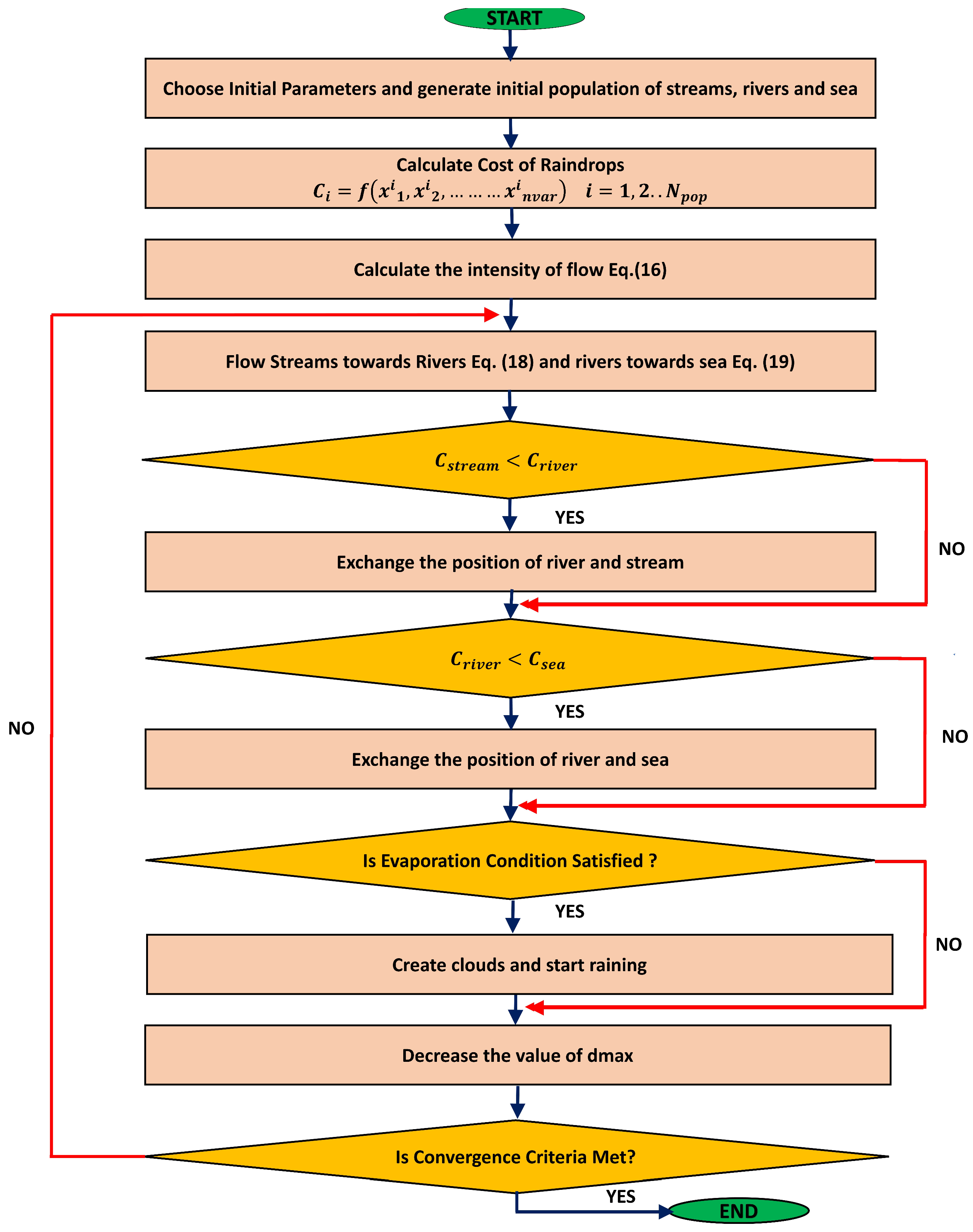
3. Water Cycle Algorithm

The water cycle is an evolutionary algorithm proposed by Ali Sadollah [34]. It is based on the natural water cycle and the downhill flow of rivers and streams toward the sea. In a natural water cycle, water is evaporated and clouds are formed through the process of condensation. After that, water comes down to earth through the process of rain. This water then takes the form of rivers and streams and is evaporated again, and this whole cycle is repeated. In WCA, solutions are termed as ‘raindrops’. Initially, the raining process is assumed. The raindrops that give the best and good fitness values are designated as ‘sea’ and ‘rivers’, respectively. The rest of the solutions are designated as ’streams’. According to the magnitude of flow, streams are absorbed by the rivers which eventually fall into the sea (the global best). The flowchart of WCA is illustrated by Figure 3. The steps of WCA are explained in the following subsections.

3.1. Generation of Initial Population

For initiation of the algorithm, the initial random population of the raindrops is generated. For an optimization problem with a number of variables N v a r , the initial solution vector (raindrop) with dimensions 1 × N v a r is represented by Equation (12).
R 1 × N v a r = [ r 1 r 2 r 3 r N v a r ]
For a population size of N p o p , the initial solution matrix with dimensions N p o p × N v a r is generated, and it is modeled in Equation (13).
R ( N p o p , N v a r ) = r 1 , 1 r 1 , 2 r 1 , N v a r r 2 , 1 r 2 , 2 r 2 , N v a r r N p o p , 1 r N p o p , 2 r N p o p , N v a r

3.2. Evaluation of Fitness Function

For each raindrop r, the fitness function value is evaluated by
F F i = F F ( r 1 , r 2 , r 3 , , r N v a r )
The number of rivers, denoted as n r , is chosen by the user. The rest of the raindrops are chosen as streams. The quantity N s r , defined in Equation (15), is equal to the sum of the rivers and sea (1 represents sea).
N s r = n r + 1
The number of streams denoted by N s is given using Equation (16).
N s = N p o p N s r

3.3. Allocation of Streams to Rivers and Sea

Streams are allocated to respective rivers and sea based on their magnitude of flow given by Equation (17).
N S i = r o u n d { | C o s t i n = 1 N s r C o s t n | } × N s
where i = 1 , 2 , , N s r · C o s t i is the value of the objective function evaluated at specific rivers and the sea. N S i is the number of streams, which move toward specific rivers and the sea.

3.4. Position Update

The flow of streams toward rivers and rivers toward the sea is along a straight line, which connects them. The length of the line is a randomly chosen distance Z, which is given in Equation (18).
Z ϵ ( 0 , C × d )
where C ranges between [1, 2] and it is usually taken as 2. The value of C being greater than unity makes the streams able to flow toward rivers in different directions. d is the current distance between the river and stream. Based on the above principle of flow, the updated positions of streams are given by Equation (19).
S j + 1 = S j + r a n d × C × ( R j S j )
where S j and S j + 1 are the current and updated positions of the stream, respectively. R j is the position of river at j-th iteration. The updated position of the river is given by Equation (20) as
R j + 1 = R j + r a n d × C × ( S e a j R j )
where R j and R j + 1 are the current and updated positions of the river, respectively. S e a j represents the position of the sea.

3.5. Evaporation Condition

The condition of evaporation helps to prevent becoming trapped in the local optima. If the distance between sea and river is less than a pre-defined value d m a x , the process of rain starts. d m a x is a small number close to zero. Its impact on the global optimal search is that the large value of d m a x hinders the search, while its small value encourages the search closer to the sea [34]. Its value successively decreases after each iteration. The raining process occurs after evaporation.

3.6. Formation of New Streams

The locations of the newly formed streams are given by Equation (21).
S n e w = L B + r a n d × ( U B L B )
where S n e w is the position of new streams, which directly flow to the sea. Equation (22) is used to generate streams whose flow is aimed directly toward the sea. This enhances the exploration near the optimal point in the feasible region for constrained problems.
S n e w = S e a + ν × r a n d n ( 1 , N v a r )
where ν shows the searching region range near the optimal point. In the majority of cases, the value of ν is taken to be 0.1.

4. Simulation Setup

WCA is used to solve the fitness function to find the optimal switching angles such that the 5th and 7th harmonics are eliminated while the fundamental frequency is kept to a fixed value. MATLAB is used to implement WCA for SHE in a PC with Intel (R) Core™, i7, 2.7 GHz CPU and 8.00 GB RAM. Solutions obtained through WCA are compared with those obtained using PSO and FA. Parameters such as population size, number of iterations, and number of runs are kept same for the three algorithms for comparison. The parameters used for these algorithms are listed in Table 1.
Matlab-Simulink is used to perform simulation for a 7-level CHBMLI. To observe the effects of optimized switching angles on the eliminated harmonics, FFT analysis is also performed. The maximum DC voltage is selected as 300 V. Figure 4 explains the working flow of WCA with CHBMLI.
The phase and line voltage waveforms obtained corresponding to modulation index 0.8 are shown in Figure 5. FFT analysis is than performed in SIMULINK to determine the percentages of eliminated harmonics with respect to fundamental. Figure 6 shows the result of the FFT analysis of the line voltage corresponding to a modulation index of 0.8.

5. Results and Analysis

This section presents results and analysis on the selection of the switching angles, analysis of the percentage of the eliminated harmonics, and the convergence behavior of the algorithms while finding the solution. Moreover, due to the stochastic nature of the meta-heuristic optimization algorithms, different statistical tests are suggested to compare the performance of each algorithm statistically over a defined sample set. Figure 7 shows optimal switching angles obtained using WCA against different values of modulation index. From the given figure, it is evident that the value of the optimum solution set, comprising different switching angles, converges to a lower value with the increase in the value of the modulation index. ψ 1 , ψ 2 , and ψ 3 represent the switching angles at different values of the modulation index. Figure 8 shows the percentages of eliminated harmonics with respect to the fundamental against different values of the modulation index. From the given bar graph, it is clear that WCA outperforms PSO and FA by giving lower values of the harmonic percentage for CHBMLI. Moreover, the performance of FA and PSO is comparable, giving optimal results at different values of the modulation index. It is also obvious that the percentage of the 5th harmonic at different values of the modulation index dominates the 7th harmonic content in the overall harmonics percentage.

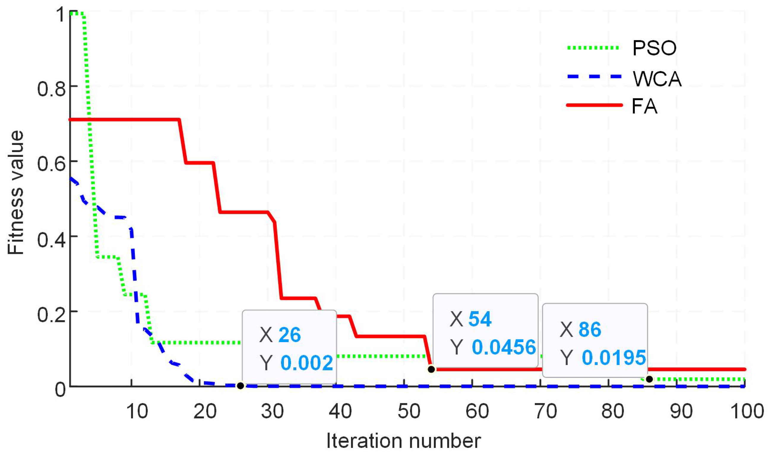
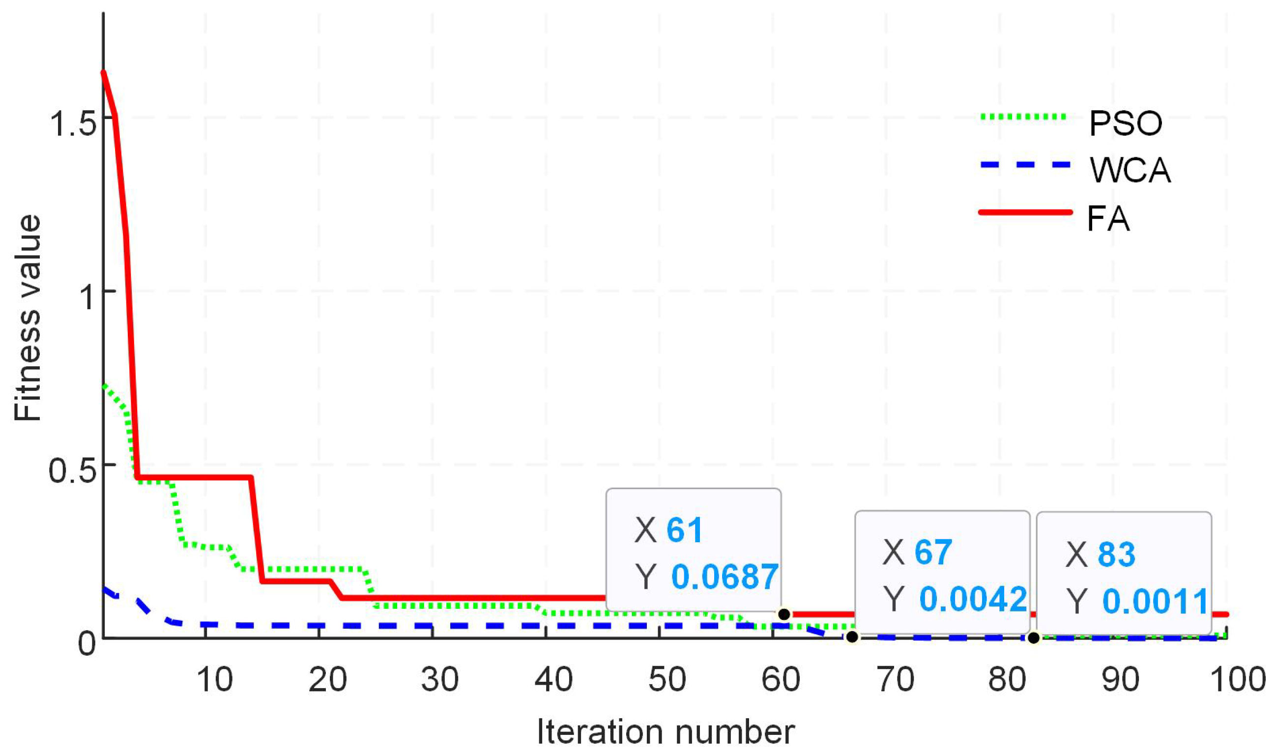
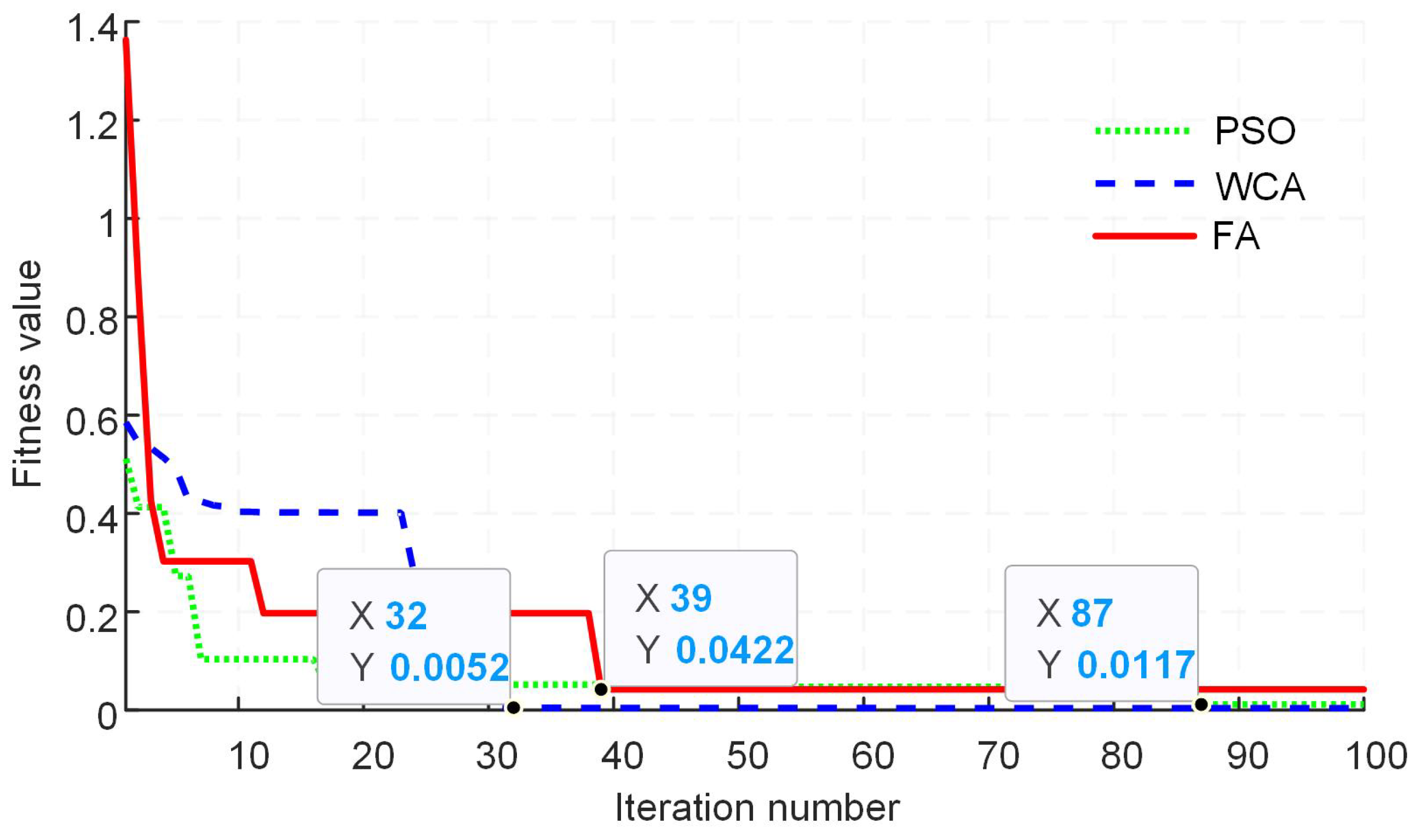
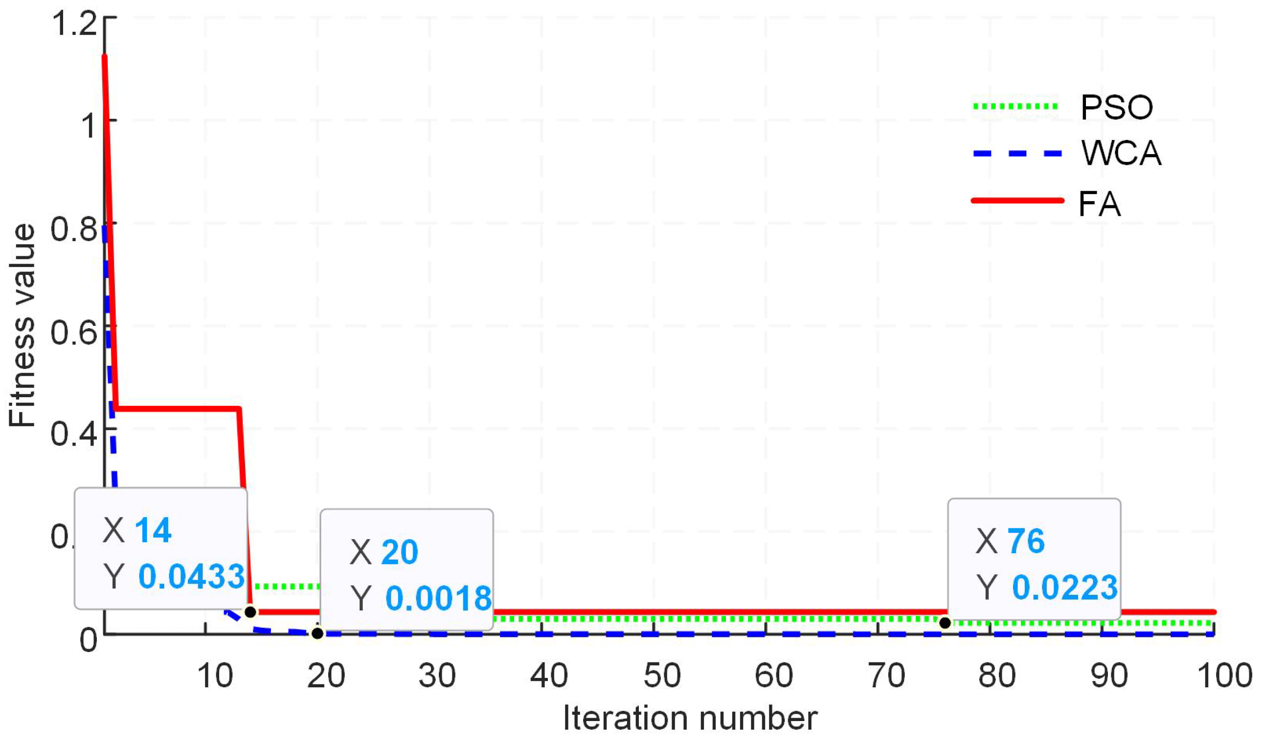
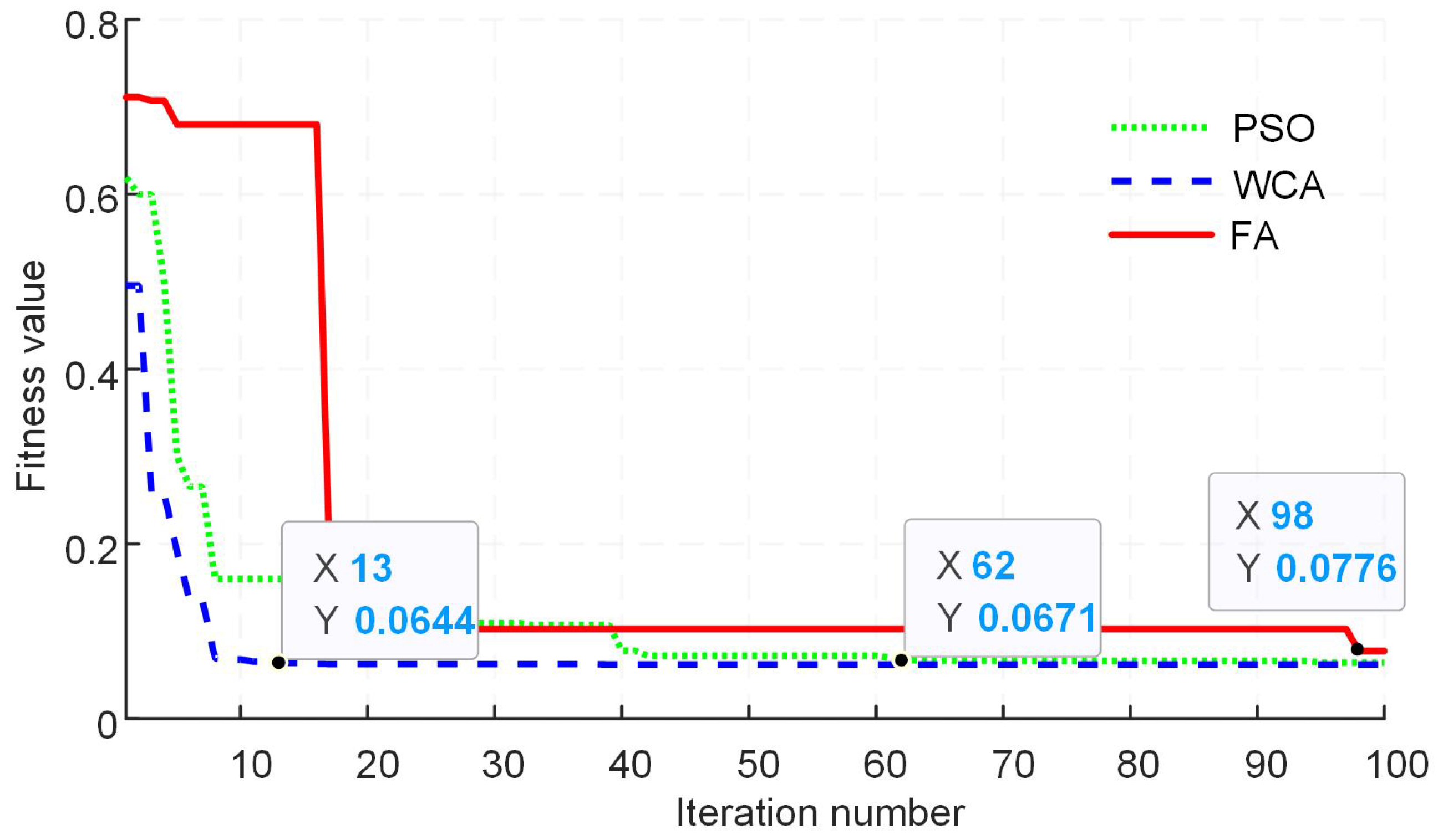
5.1. Convergence Analysis
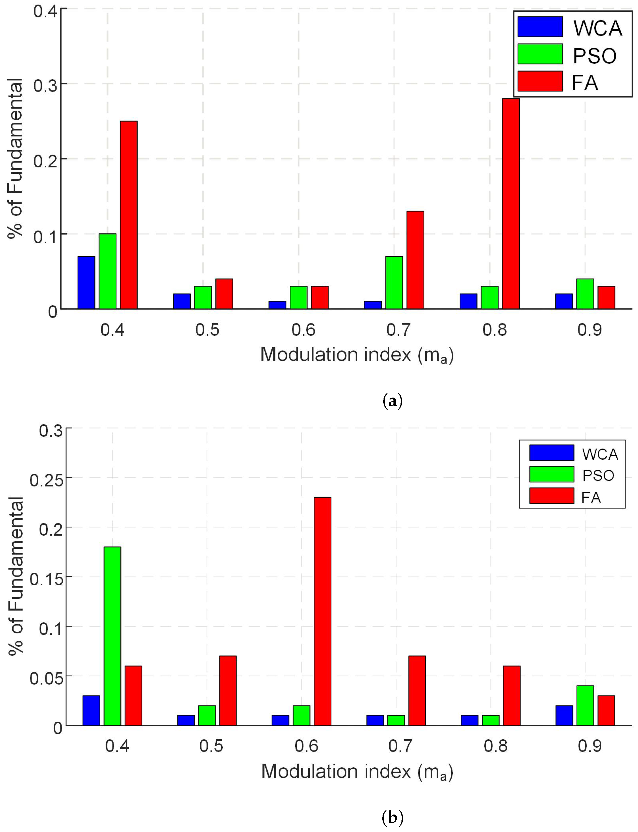
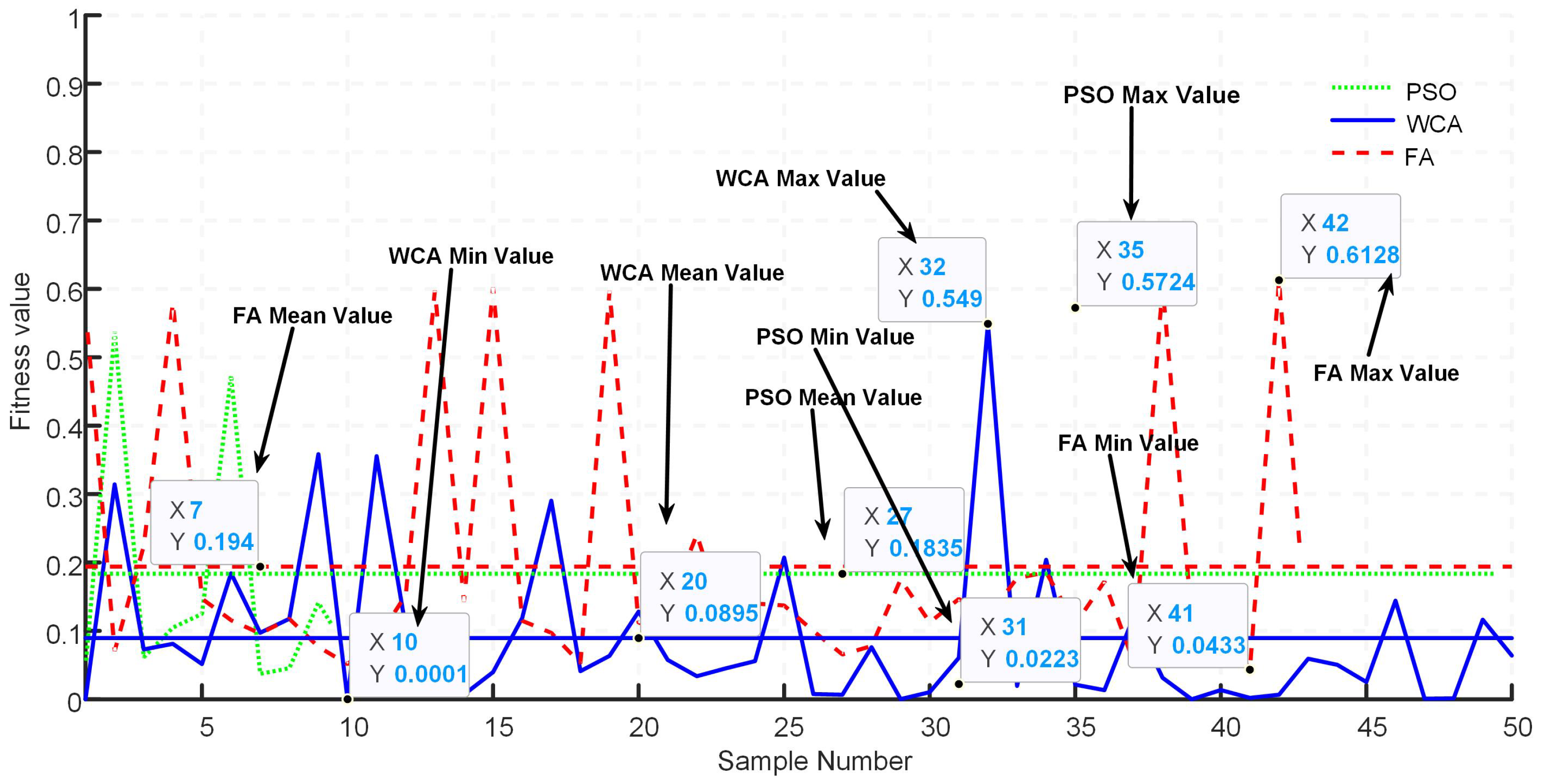
In order to obtain the convergence characteristic comparison, each meta-heuristic optimization algorithm is tested at different values of the modulation index. Further, the total number of iterations is kept at 100 for each algorithm, and the population size used is selected as 50 particles/fireflies or rain drops. Figure 9, Figure 10, Figure 11, Figure 12, Figure 13 and Figure 14 show the results of the fitness value comparison of different algorithms against the modulation index values. From the given graphs, it can be observed that WCA outperforms the remaining algorithms by giving a lower fitness value. Moreover, WCA also converges to an optimal solution in fewer iterations. FA tends to become trapped in the local optima as the value of the modulation index increases.

5.2. Fitness Values

The maximum, minimum and mean values obtained by the three algorithms for all modulation indexes for 50 runs are given in Table 2. It can be observed that the mean value obtained by WCA for 50 samples over all modulation indexes is less as compared to PSO and FA.
Figure 15 illustrates a graphical representation of the minimum, maximum and average fitness values obtained by the three algorithms for a modulation index of 0.8 over 50 samples. It is evident that the mean value obtained by WCA is less than that of PSO and FA over 50 samples. Moreover, the minimum value found by WCA over 50 samples is 0.0001, whereas those of PSO and FA are 0.0223 and 0.0433, which shows that WCA has better accuracy while finding the optimal solution.

5.3. Statistical Results

Meta-heuristic algorithms have a random nature. Due to this random nature, we obtain different results after each run. So, for comparing the performance of two metaheuristic algorithms, some statistics-based methods are used over a fixed sample size. In this research, we compare the average fitness value obtained by the algorithms for different population sizes, and to statistically differentiate them, we employ independent sample t-test results. The independent sample t-test has two parts: one is Levene’s test, which plays a role in the comparison of variances, and the second is the t-test, which is responsible for the comparison of means.
According to Levene’s test and the t-test, for the results to be statistically different for the 95% confidence interval, the significant value should be smaller than the critical value of 0.05. In the case of the statistical comparison between PSO and WCA, we can see from Table 3 that for the population sizes of 20, 35 and 50, the significant values for both the t-test and Leven test of inequality, are less than 0.05, which means that the results obtained through WCA and PSO are statistically different for these population sizes. The execution time of WCA is more than that of PSO. In the case of FA and WCA, for a population size of 20, the t-test significant value is less than 0.05, so we can say that means are different, whereas variances are same. The same applies in the case for a population size of 35. It can be seen from Table 4 that the execution time of WCA is less than that of FA.

6. Conclusions

The water cycle algorithm is easy to implement, as it has only one tuning parameter as compared to particle swarm optimization and firefly algorithms. The water cycle algorithm gave competitive results compared to particle swam optimization and firefly algorithms for harmonic elimination in a seven-level cascaded H-bridge multi-level inverter. It also converges to the optimal solution in less number of iterations and its accuracy is better. The mean fitness value achieved by water cycle algorithm over 50 samples is less as compared to particle swarm optimization and firefly algorithms. For most of the population sizes, results obtained through water cycle algorithm are better from those obtained through particle swarm optimization and firefly algorithms. The drawback of WCA is the initial tuning and online tuning with faults, which needs to be further studied. In future, the application of water cycle algorithm can be applied for solving SHE equations for harmonic elimination in higher-level inverters.

Author Contributions

Conceptualization, M.K., U.T.S., M.F.Z., Y.A. and M.B.; methodology, M.K., M.F.Z. and Y.A.; software, M.K. and M.F.Z.; validation, M.K., U.T.S., M.F.Z., Y.A. and M.B.; formal analysis, M.K., U.T.S., M.F.Z. and Y.A.; writing—original draft preparation, M.K., M.F.Z. and Y.A.; writing—review and editing, M.K., U.T.S., M.F.Z., Y.A. and M.B. All authors have read and agreed to the published version of the manuscript.

Funding

This research received no external funding.

Institutional Review Board Statement

Not applicable.

Informed Consent Statement

Not applicable.

Data Availability Statement

All data are provided in this manuscript.

Conflicts of Interest

The authors declare no conflict of interest.

Nomenclature

The following abbreviations and notations are used in this manuscript:
Abbreviations
CHBMLICascaded H-Bridge Multilevel Inverter
EMIElectromagnetic Interference
FAFirefly Algorithm
MLIMultilevel Inverter
PSOParticle Swarm Optimization
RESRenewable Energy Systems
SHESelective Harmonic Elimination
WCAWater Cycle Algorithm
NRNewton–Raphson
BABee Algorithm
GAGenetic Algorithm
CSACuckoo Search Algorithm
BOABat Optimization Algorithm
ACOAnt Colony Optimization
GWOGrey Wolf Optimizer
MGWOModified Grey Wolf Optimizer
SSASalt Swarm Algorithm
 
Notations
V d c DC Voltage applied to H–Bridge Cell
V 1 Fundamental component
F F Fitness function
m a Modulation index
N p o p Population size
N v a r Number of variables
n r Number of rivers
N s Number of streams
N s r Sum of sea and rivers
N S i Number of streams allocated to particular sea or rivers
dCurrent distance between stream and river
S j Current position of stream at j-th
S j + 1 Updated position of stream at j + 1 iteration
R j Current position of river at j-th
R j + 1 Updated position of river at j + 1 iteration
S n e w Position of new streams which directly flow towards sea
L B Lower bound
U B Upper bound

References

  1. Ali, M.; Din, Z.; Solomin, E.; Cheema, K.M.; Milyani, A.H.; Che, Z. Open switch fault diagnosis of cascade H-bridge multi-level inverter in distributed power generators by machine learning algorithms. Energy Rep. 2021, 7, 8929–8942. [Google Scholar] [CrossRef]
  2. Flourentzou, N.; Agelidis, V.G.; Demetriades, G.D. VSC-based HVDC power transmission systems: An overview. IEEE Trans. Power Electron. 2009, 24, 592–602. [Google Scholar] [CrossRef]
  3. Song, Q.; Liu, W. Control of a cascade STATCOM with star configuration under unbalanced conditions. IEEE Trans. Power Electron. 2009, 24, 45–58. [Google Scholar] [CrossRef]
  4. Sadigh, A.K.; Hosseini, S.H.; Sabahi, M.; Gharehpetian, G.B. Double flying capacitor multicell converter based on modified phase-shifted pulsewidth modulation. IEEE Trans. Power Electron. 2009, 25, 1517–1526. [Google Scholar] [CrossRef]
  5. Hatti, N.; Hasegawa, K.; Akagi, H. A 6.6-kV transformerless motor drive using a five-level diode-clamped PWM inverter for energy savings of pumps and blowers. IEEE Trans. Power Electron. 2009, 24, 796–803. [Google Scholar] [CrossRef]
  6. Nami, A.; Zare, F.; Ghosh, A.; Blaabjerg, F. A hybrid cascade converter topology with series-connected symmetrical and asymmetrical diode-clamped H-bridge cells. IEEE Trans. Power Electron. 2009, 26, 51–65. [Google Scholar] [CrossRef] [Green Version]
  7. Kumar, P.; Kour, M.; Goyal, S.K.; Singh, B.P. Multilevel inverter topologies in renewable energy applications. In Intelligent Computing Techniques for Smart Energy Systems; Springer: Berlin/Heidelberg, Germany, 2020; pp. 891–902. [Google Scholar]
  8. Benyamina, F.; Benrabah, A.; Khoucha, F.; Zia, M.F.; Achour, Y.; Benbouzid, M. An augmented state observer-based sensorless control of grid-connected inverters under grid faults. Int. J. Electr. Power Energy Syst. 2021, 133, 107222. [Google Scholar] [CrossRef]
  9. Zia, M.; Elbouchikhi, E.; Benbouzid, M. An energy management system for hybrid energy sources-based stand-alone marine microgrid. In IOP Conference Series: Earth and Environmental Science; IOP Publishing: Bristol, UK, 2019; Volume 322, p. 012001. [Google Scholar]
  10. Janardhan, K.; Mittal, A.; Ojha, A. Performance investigation of stand-alone solar photovoltaic system with single phase micro multilevel inverter. Energy Rep. 2020, 6, 2044–2055. [Google Scholar] [CrossRef]
  11. Abbasi, M.A.; Zia, M.F. Novel TPPO based maximum power point method for photovoltaic system. Adv. Electr. Comput. Eng. 2017, 17, 95–100. [Google Scholar] [CrossRef]
  12. Memon, M.A.; Mekhilef, S.; Mubin, M.; Aamir, M. Selective harmonic elimination in inverters using bio-inspired intelligent algorithms for renewable energy conversion applications: A review. Renew. Sustain. Energy Rev. 2018, 82, 2235–2253. [Google Scholar] [CrossRef]
  13. Liang, T.J.; O’Connell, R.M.; Hoft, R.G. Inverter harmonic reduction using Walsh function harmonic elimination method. IEEE Trans. Power Electron. 1997, 12, 971–982. [Google Scholar] [CrossRef]
  14. Aghdam, G.H. Optimised active harmonic elimination technique for three-level T-type inverters. IET Power Electron. 2013, 6, 425–433. [Google Scholar] [CrossRef]
  15. Kumar, J.; Das, B.; Agarwal, P. Harmonic reduction technique for a cascade multilevel inverter. Int. J. Recent Trends Eng. 2009, 1, 181. [Google Scholar]
  16. Sun, J.; Grotstollen, H. Solving nonlinear equations for selective harmonic eliminated PWM using predicted initial values. In Proceedings of the 1992 International Conference on Industrial Electronics, Control, Instrumentation, and Automation, San Diego, CA, USA, 13 November 1992; pp. 259–264. [Google Scholar]
  17. Imarazene, K.; Chekireb, H. Selective harmonics elimination PWM with self-balancing DC-link in photovoltaic 7-level inverter. Turk. J. Electr. Eng. Comput. Sci. 2016, 24, 3999–4014. [Google Scholar] [CrossRef]
  18. Yang, K.; Zhang, Q.; Yuan, R.; Yu, W.; Yuan, J.; Wang, J. Selective harmonic elimination with Groebner bases and symmetric polynomials. IEEE Trans. Power Electron. 2015, 31, 2742–2752. [Google Scholar] [CrossRef]
  19. Zheng, C.; Zhang, B. Application of Wu method to harmonic elimination techniques. Proc. CSEE 2005, 25, 40–45. [Google Scholar]
  20. Chiasson, J.N.; Tolbert, L.M.; McKenzie, K.J.; Du, Z. Elimination of harmonics in a multilevel converter using the theory of symmetric polynomials and resultants. IEEE Trans. Control. Syst. Technol. 2005, 13, 216–223. [Google Scholar] [CrossRef]
  21. Chiasson, J.N.; Tolbert, L.M.; Du, Z.; McKenzie, K.J. The use of power sums to solve the harmonic elimination equations for multilevel converters. EPE J. 2005, 15, 19–27. [Google Scholar] [CrossRef]
  22. Al-Othman, A.; Ahmed, N.A.; AlSharidah, M.; AlMekhaizim, H.A. A hybrid real coded genetic algorithm–pattern search approach for selective harmonic elimination of PWM AC/AC voltage controller. Int. J. Electr. Power Energy Syst. 2013, 44, 123–133. [Google Scholar] [CrossRef]
  23. Reza Salehithe, R.; Farokhnia, N.; Abedi, M.; Fathi, S. Elimination of low order harmonics in multilevel inverters using genetic algorithm. J. Power Electron. 2011, 11, 132–139. [Google Scholar]
  24. Shen, K.; Zhao, D.; Mei, J.; Tolbert, L.M.; Wang, J.; Ban, M.; Ji, Y.; Cai, X. Elimination of harmonics in a modular multilevel converter using particle swarm optimization-based staircase modulation strategy. IEEE Trans. Ind. Electron. 2014, 61, 5311–5322. [Google Scholar] [CrossRef]
  25. Kavousi, A.; Vahidi, B.; Salehi, R.; Bakhshizadeh, M.K.; Farokhnia, N.; Fathi, S.H. Application of the bee algorithm for selective harmonic elimination strategy in multilevel inverters. IEEE Trans. Power Electron. 2011, 27, 1689–1696. [Google Scholar] [CrossRef]
  26. Ajami, A.; Mohammadzadeh, B.; Oskuee, M.R.J. Utilizing the cuckoo optimization algorithm for selective harmonic elimination strategy in the cascaded multilevel inverter. ECTI Trans. Electr. Eng. Electron. Commun. 2014, 12, 7–15. [Google Scholar]
  27. Ganesan, K.; Barathi, K.; Chandrasekar, P.; Balaji, D. Selective harmonic elimination of cascaded multilevel inverter using BAT algorithm. Procedia Technol. 2015, 21, 651–657. [Google Scholar] [CrossRef] [Green Version]
  28. Karthik, N.; Arul, R. Harmonic elimination in cascade multilevel inverters using Firefly algorithm. In Proceedings of the 2014 International Conference on Circuits, Power and Computing Technologies (ICCPCT-2014), Nagercoil, India, 20–21 March 2014; pp. 838–843. [Google Scholar]
  29. Babaei, M.; Rastegar, H. Selective harmonic elimination PWM using ant colony optimization. In Proceedings of the 2017 Iranian Conference on Electrical Engineering (ICEE), Tehran, Iran, 2–4 May 2017; pp. 1054–1059. [Google Scholar]
  30. Dzung, P.Q.; Tien, N.T.; Tuyen, N.D.; Lee, H.H. Selective harmonic elimination for cascaded multilevel inverters using grey wolf optimizer algorithm. In Proceedings of the 2015 9th International Conference on Power Electronics and ECCE Asia (ICPE-ECCE Asia), Seoul, Korea, 1–5 June 2015; pp. 2776–2781. [Google Scholar]
  31. Routray, A.; Singh, R.K.; Mahanty, R. Harmonic reduction in hybrid cascaded multilevel inverter using modified grey wolf optimization. IEEE Trans. Ind. Appl. 2019, 56, 1827–1838. [Google Scholar] [CrossRef]
  32. Babu, T.S.; Priya, K.; Maheswaran, D.; Kumar, K.S.; Rajasekar, N. Selective voltage harmonic elimination in PWM inverter using bacterial foraging algorithm. Swarm Evol. Comput. 2015, 20, 74–81. [Google Scholar] [CrossRef]
  33. Hosseinpour, M.; Mansoori, S.; Shayeghi, H. Selective Harmonics Elimination Technique in Cascaded H-Bridge Multi-Level Inverters Using the Salp Swarm Optimization Algorithm. J. Oper. Autom. Power Eng. 2020, 8, 32–42. [Google Scholar]
  34. Eskandar, H.; Sadollah, A.; Bahreininejad, A.; Hamdi, M. Water cycle algorithm—A novel metaheuristic optimization method for solving constrained engineering optimization problems. Comput. Struct. 2012, 110, 151–166. [Google Scholar] [CrossRef]
Figure 1. Multi-level inverter for distributed energy resources-based smart grid system.
Machines 10 00399 g001
Figure 2. Stepped waveform for a 7-level inverter.
Machines 10 00399 g002
Figure 3. Flowchart illustrating working of water cycle algorithm.
Machines 10 00399 g003
Figure 4. Working flow of water cycle algorithm with CHBMLI.
Machines 10 00399 g004
Figure 5. (a) Phase voltage and (b) line voltage for m a = 0.8.
Machines 10 00399 g005
Figure 6. FFT Analysis.
Machines 10 00399 g006
Figure 7. Switching angles for different values of modulation index.
Machines 10 00399 g007
Figure 8. Percentages of eliminated harmonics against each modulation index ( m a ). (a) Contribution of 5th harmonic, (b) contribution of 7th harmonic.
Machines 10 00399 g008
Figure 9. Fitness value comparison of different algorithms for modulation index value of 0.4.
Machines 10 00399 g009
Figure 10. Fitness value comparison of different algorithms for modulation index value of 0.5.
Machines 10 00399 g010
Figure 11. Fitness value comparison of different algorithms for modulation index value of 0.6.
Machines 10 00399 g011
Figure 12. Fitness value comparison of different algorithms for modulation index value of 0.7.
Machines 10 00399 g012
Figure 13. Fitness value comparison of different algorithms for modulation index value of 0.8.
Machines 10 00399 g013
Figure 14. Fitness value comparison of different algorithms for modulation index value of 0.9.
Machines 10 00399 g014
Figure 15. Fitness value for 50 runs.
Machines 10 00399 g015
Table 1. Algorithm parameters.
AlgorithmParameter
WCAPopulation size20
Iterations100
Number of Rivers4
d m a x 0.001
Number of Runs50
PSOPopulation Size20
Iterations100
c1,c22
Number of Runs50
FAPopulation Size20
Iterations100
Attractiveness Co-efficient1
Randomization parameter0.5
Absorption Co-efficient1
Number of Runs50
Table 2. Maximum, minimum, and mean fitness values obtained by algorithms.
m a AlgorithmFF Value
MaxMinMean
0.4PSO0.67280.0140.1257
FA0.33120.03610.1266
WCA0.2982.08 × 10−50.05
0.5PSO0.370.0130.081
FA0.210.0010.12
WCA0.350.0010.06
0.6PSO0.33160.0120.08
FA0.17030.030.1
WCA0.18670.00010.05
0.7PSO0.48210.02190.1514
FA0.35610.030.1506
WCA0.26180.00010.101
0.8PSO0.57380.0160.16
FA0.64840.030.238
WCA0.36790.00010.0823
0.9PSO0.86290.06760.1729
FA0.88710.07610.2016
WCA0.46470.05580.0912
Table 3. Statistical comparison between WCA and PSO for 50 samples.
Size of PopulationAvg. Fitness ValueMax Fitness ValueMin Fitness ValueAvg. Execution Time (Sec)Sig. Values for Each Test
PSOWCAPSOWCAPSOWCAPSOWCAt-TestLevene’s Test
50.33410.40370.68350.84360.020.040.0150.050.2960.398
200.22330.17210.45370.5490.0330.00050.04510.10320.0010.003
350.11960.06320.37890.13440.0330.00030.06790.28170.0040.006
500.11960.04110.39190.11990.020860.00020.1240.38170.0120.04
Table 4. Statistical comparison between WCA and FA for 50 samples.
Size of PopulationAvg. Fitness ValueMax Fitness ValueMin Fitness ValueAvg. Execution Time (Sec)Sig. Values for Each Test
FAWCAFAWCAFAWCAFAWCAt-TestLevene’s Test
50.45000.40310.75380.84360.21010.04030.050.050.8220.833
200.12040.17210.20280.5490.070.31350.20490.15230.0010.594
350.10260.06320.15600.13440.05480.00030.82510.28170.020.44
500.17070.04110.59190.11990.05890.00021.64730.38170.2150.04
Publisher’s Note: MDPI stays neutral with regard to jurisdictional claims in published maps and institutional affiliations.

